
95% of researchers rate our articles as excellent or good
Learn more about the work of our research integrity team to safeguard the quality of each article we publish.
Find out more
ORIGINAL RESEARCH article
Front. Phys. , 04 February 2022
Sec. Social Physics
Volume 10 - 2022 | https://doi.org/10.3389/fphy.2022.827929
This article is part of the Research Topic Data-driven Modeling and Optimization: Applications to Social Computing View all 25 articles
 Gui-Quan Sun1,2*
 Yizhi Pang2
 Li Li3
 Chen Liu4*
 Yongping Wu5
 Guolin Feng5,6
 Zhen Jin2
 Bai-Lian Li7
 Zhen Wang8*
Pattern structures are usually used to describe the spatial and temporal distribution characteristics of individuals. However, the corresponding relationship between the pattern structure and system robustness is not well understood. In this work, we use geostatistical method–semivariogram to study system robustness for different pattern structures based on three dynamical models in different fields. The results show that the structural ratio of different pattern structures including the mixed state of spot and stripe, cold spot, stripe only, and hot spot are more than 75%, which indicated those patterns all have strong spatial dependence and heterogeneity. It was revealed that the systems corresponding to the mixed state of spot and stripe or cold spot are more robust. This article proposed a method to characterize the robustness of the system corresponding to the pattern structure and also provided a feasible approach for the study of “how structures determine their functions.”
Due to some behavior mechanisms of individuals, species present heterogeneous but regular spatial distribution structures in both space and time, which is called as “pattern.” These pattern structures exist widely in nature such as the clouds in the sky [1], the patterns on zebra [2], and the ripples on the water [3]. Except for these, Getzin et al. found the gap vegetation pattern—fairy circles in Western Australia [4], the regular stripes vegetation distribution on the hillside of Niger studied by Klausmeier et al. [5], and mussel beds in the intertidal zone show different scales of distribution, namely, large-scale banded distribution at the ecological level and small-scale reticular distribution at individual mussels level [6, 7]. There are also thermal convection patterns, spiral wave patterns, and hexagonal patterns observed in the experiment [8, 9].
The scientific community has a wide range of interest in the formation mechanism and structural characteristics behind the pattern. Consequently, theories of pattern dynamics have been deeply studied and form a more systematic theoretical research area [10–21]. Here, we present some typical works on this topic. In 2001, von Hardenberg et al. pointed out that when the bare state and spot pattern state coexist, and it is also unstable, if exceeding a certain threshold, the system will be completely transformed to a bare state or desertification, that is, the spotted pattern will be used as an early warning signal of desertification [22]. In 2014, Liu et al. revealed that the interaction of self-organization behavior between different scales can improve the robustness, persistence and productivity of mussel ecosystem; in other words, the mosaic patterns with large and small scales imply the ecosystem is more robust [6]. In 2020, Bastiaansen et al. quantified the resilience of ecosystems with spatial patterns by using phase portrait [23]. However, due to the complexity of the system dynamical process and the lack of uniformity on robustness definition, many studies and conclusions are not comprehensive and have certain limitations, even lack of quantitative indicators for the robustness of each pattern structure.
In order to better answer the question “how the pattern structures determine the robustness of the system,” we obtain a series of different pattern structures based on three dynamical models in different research fields: vegetation–water coupled model [24], epidemic spatial model [25], and predator–prey model [26], and use geostatistical methods to quantitatively describe and analyze the characteristics of all different pattern structures, so as to find out which type of pattern structures are more robust for the corresponding systems.
In ecology, the related concepts of robustness is complicated and imprecise, but most people agree that robustness can be divided into two categories: one is the ability of the system to resist leaving (maintain) the current state after the system is subjected to external disturbance [27]; the other one is the ability of the system to return to the original stable state after suffering disturbance [28]. Therefore, in this study, we will use semi-variogram to analyze the interaction and dependence of each component within the system, and thereby give the quantitative index of the second type of system robustness.
The semivariogram is a mathematical statistical method that can reflect the randomness and structural characteristics of the variable in the spatial distribution and also is the theoretical basis of geostatistics. First, in order to avoid the proportional effect in the study, it is necessary to test the data of the studied variable (Z) and judge whether it is normal distribution or approximate normal distribution; if not, data conversion shall be carried out to make it conform to normal distribution. Afterward, the calculation of the semi-variance function value is carried out. Finally, through simulation, we obtain the best fitted semivariogram model and some important indicators, such as nugget C0, sill C0 + C, range A, and the structural ratio C/(C0 + C). Figure 1 shows the basic process of this method and the calculation formula of the semivariogram as follows [29]:
where γ(h) represents semivariogram, h is the step length, that is the sample point spatial distance, N(h) indicates the total number of data pairs when the sample point distance is h, and Z (xi) and Z (xi+h), respectively, are the values of the variable(Z) at the spatial position xi and xi+h.
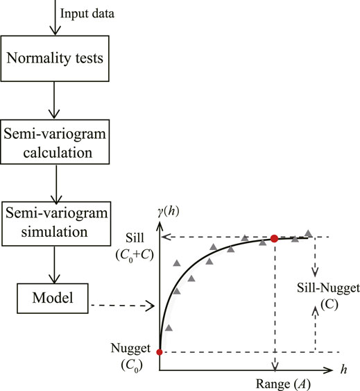
FIGURE 1. Flowchart of quantitative system robustness index [30]. The analysis of semivariogram is mainly divided into three phases: normal test of research data, calculation of the semi-variance of variable, and simulation semivariogram to obtain the best fitted model. Structural ratio C/(C0 + C) can reflect the robustness of the system.
In Figure 1, the nugget C0 represents the degree of random heterogeneity of variables in the region and the sill (C0 + C) refers to the maximum variation of the system induced by structural variation and random variation. Then, the structural ratio C/(C0 + C) indicates the contribution rate of structural factors to spatial heterogeneity, which can reflect the spatial dependence and the spatial heterogeneity of variables [31]. When the structural ratio is less than 25%, it indicates that the variable has weak spatial dependence; if 25% ≤ structural ratio
In arid and semi-arid areas, vegetation growth is mainly limited by water resources [5]. In 2004, Gilad et al. considered three feedback mechanisms between vegetation biomass and water resources, infiltration feedback, root augmentation feedback, and soil–water diffusion feedback mechanism (Figure 2), and established a dynamical model for coupling a single vegetation species with water [34, 35]. On this basis, scholars made the following assumptions: 1) the lateral extension of vegetation roots is restricted and 2) the infiltration rate of bare soil and vegetation covered area is the same, and then obtained a simplified dimensionless model as follows [24]:
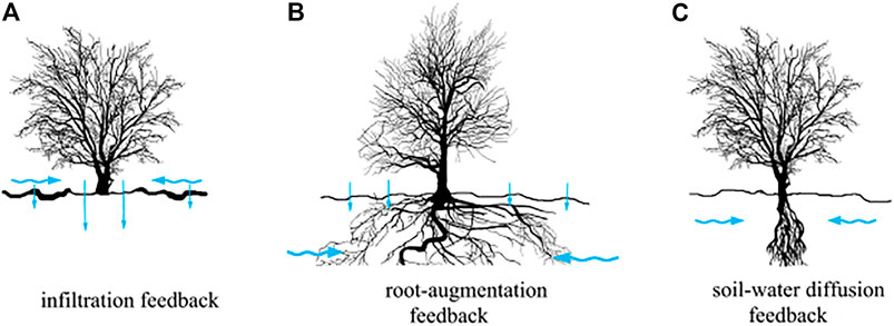
FIGURE 2. Schematic diagram of three feedback mechanisms between vegetation and water. (A) Difference of infiltration rate between bare soil and vegetation covered area causes surface water flow, (B) vegetation roots extend laterally to absorb water, and (C) soil water diffusivity exceed the spread of vegetation biomass. The blue arrow indicates the direction of water flow, and the length of the straight arrow represents the size of infiltration rate.
In the previous dimensionless model, the biological significances and values of all parameters are shown in Table 1. Next, we study the influence of the shading rate ρ on the robustness of vegetation ecosystems. Fixing other parameters, through numerical simulation, we get a series of vegetation pattern structure, as shown in Figure 3.
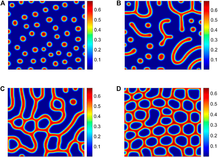
FIGURE 3. Vegetation pattern structure under different shading rates ρ. (A) Hot spot pattern with ρ = 0.6; (B) spots–stripes mixed pattern with ρ = 0.75; (C) stripe pattern with ρ = 0.9; (D) cold spot pattern with ρ = 0.94. See Table 1 for the other parameter values.
For the previous four different vegetation patterns, hot spot, mixed spots and stripes, stripe, and cold spot, we use vegetation density as a research variable and perform a semi-variogram analysis on them. According to Table 2, it is found that the structural ratio C/(C0 + C) of these four vegetation patterns in descending order are as follows: mixed spots and stripes
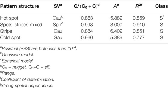
TABLE 2. Fitted semivariogram models (SV) and their characteristic parameters for different vegetation pattern structures (Figure 3). The high value of R2 and the low of RSS indicate good fitted effect.
The spread of infectious diseases will be affected by the spatial movement of the susceptible or infected, which will eventually lead to spatial patterns of the susceptible and infected individuals [37, 38]. In view of the characteristics of acquired immunodeficiency Syndrome (AIDS), hepatitis B virus (HBV), ebola virus, and other infectious diseases that are difficult to be cured after infected, meanwhile considering the complex spatial dynamics of the susceptible and the infected, scholars proposed an epidemic spatial model with non-linear incidence rates [25]. The non-linear incidence rate is caused by twice exposures of susceptible before infection. The transmission mechanism of such infectious disease can be described in Figure 4. The biological significances and values of all parameters in the model are shown in Table 3. The specific mathematical model is as follows:

FIGURE 4. Schematic diagram of infectious diseases transmission process. The model satisfies the following conditions: 1) the epidemic cannot be cured after being infected; 2) the susceptible is exposed to the disease repeatedly, leading to a non-linear transmission rate.
Based on the spatial infectious disease model (3), we studied the impact of the spatial distribution of infected individuals on the spread of infectious diseases in the population. First, fixing other parameters, only changing the transmission rate β, and a series of numerical simulations are carried out on model (3). Finally, we get the pattern structure, as shown in Figure 5.
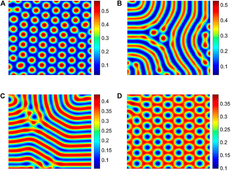
FIGURE 5. Different patterns of infected individuals. (A) Hot spot pattern with β = 32; (B) spots and stripes mixed pattern with β = 35; (C) stripe pattern with β = 40; and (D) cold spot pattern with β = 42.
With the increase in the transmission rate, the spatial distribution of infected individuals present four different pattern structures: hot spot, mixed spots and stripes, stripe, and cold spot (Figure 5). From Table 4, we find that the structural ratio C/(C0 + C) of the four different spatial distributions of the infected are all greater than 75%, and their ratios are arranged in the following order: spot–stripe mixed
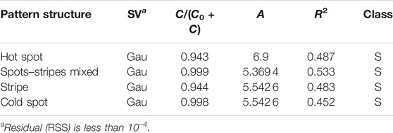
TABLE 4. Fitted semivariogram models (SV) and its characteristic parameters for different infected pattern (Figure 5). The meanings of other parameters are consistent with Table 2.
The predator function response is an indispensable part of describing the predator–prey model. This function can reflect the influence of the competition between predators on the predation efficiency, such as the coyotes, and jackrabbits in the western wilderness of North America and the plankton experiment [39]. In particular, when the predator can capture a large amount of prey per unit time, or when saturation is not considered, a ratio-dependent functional response is obtained [40]. However, with the addition of spatial diffusion, this ratio-dependent predator–prey model will produce a heterogeneous spatial distribution structure [26]. As a result, we consider this ratio-dependent predator–prey model with diffusion terms. After introducing dimensionless variables, the model is simplified to the following equations [26]
The dimensionless variables in model (4) and their values are shown in Table 5. Fixing other parameters and changing the prey consumption rate by predator γ, through numerical simulation, we obtain prey pattern structures, as shown later (Figure 6).

FIGURE 6. Different pattern structures of prey population. (A) Cold spot pattern with γ = 1.95; (B) stripe pattern with γ = 2.05.
On the basis of the previous method, we conduct a semi-variogram analysis on the previous two spatial distribution structures of prey. The detailed results are shown in Table 6. According to the heterogeneity classification standard, we find that the structural ratio C/(C0 + C) of these two patterns is significantly higher than 75%. However, by comparison, the structural ratio of the cold spot pattern is larger than that of the stripe pattern, that is, its corresponding system is more robust. Compared with the stripe structure, the cold spot pattern makes the prey to gather together and is not easy to be captured by the predators, and thus, the system is more robust.

TABLE 6. Fitted semivariogram models (SV) and its characteristic parameters for different prey pattern (Figure 6). The meanings of other parameters are consistent with Table 2.
The range A is an important index in geostatistics that can reflect the spatial heterogeneity or spatial dependence scale of regional variables. From the perspective of the range, we find that all the ranges obtained by analyzing the pattern structure above are larger than the sampling interval − − 1. Therefore, it shows that the sampling interval used in the study is credible for unbiased estimation of this area.
System robustness and pattern structure are two important characteristics to portray the spatiotemporal complexity of systems. However, the analysis of their corresponding relationship is lack of systematic research results. Focusing on the scientific problem of “which pattern structure implies the robustness of the system, and which pattern structure means the vulnerability of the system,” we combined three dynamical models from different fields, vegetation-water dynamical model [24], epidemic spatiotemporal dynamical model [25], and predator–prey spatial evolution dynamical model [26], and used geostatistical methods to analyze a series of different pattern structures produced by them. Finally, we found that the robustness of the system corresponding to different pattern structures is arranged as follows: spots and stripes mixed
In addition, we explored the systems’ resilience of different vegetation pattern structures (Figure 7), combined with the latest research methods [41]. We once again confirmed that the recovery rates of ecosystems with hot spot are the worst, compared with the other three pattern structures. And it also revealed that the recovery rate of the ecosystem corresponding to the spots and stripes mixed is greater than that of the cold spot. However, the only difference is that the recovery rate of system with stripe is the largest, which may be because the added disturbance increases the local density and finally affects the characteristics of the strip structure.
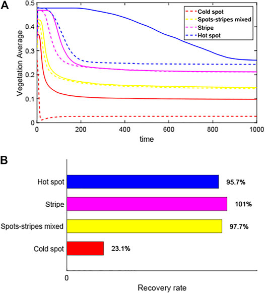
FIGURE 7. Recovery of different pattern structures for same disturbance. (A) Trajectories of different patterns when they return to steady state after the 20% disturbance occurs. Solid lines: trajectories of patterns formation; dashed lines: recovery track after the equilibrium point is reduced by 20%. (B) Recovery rates after a disturbance.
The evaluation of system robustness generally requires a large number of monitoring data or experimental data [42, 43]. However, our study is mainly based on the dynamical model to obtain the pattern structures, which can not only dynamically reflect the evolution of the system in time and space but also quantitatively predict the future spatiotemporal distribution structure. At the same time, the semi-variogram analysis method can comprehensively analyze and compare the spatial characteristics of each pattern structure, overcome the complexity of the previous analysis system robustness, and provide a new idea for describing the corresponding relationship between the pattern structure and the system robustness.
It is worth noting that our research ignores the scale dependence and does not combine with real data, while the pattern structure has different scales and can be completely corresponded to the real data. In this case, we can improve and verify our theoretical results based on GIS and big data analysis. Furthermore, the pattern structure can be divided into steady-state and non–steady-state structures, and this study only focuses on the former case. While for the non–steady-state pattern, its existence in the real world is more extensive, and hence, the correspondence between the unsteady structure and the robustness of the system is also an important scientific issue. We hope these questions will be systematically addressed in future research.
The original contributions presented in the study are included in the article/Supplementary Material; further inquiries can be directed to the corresponding authors.
All authors have made great contributions to the writing of study and approved the submitted version. G-QS, YP, LL, CL, YW, and ZW established dynamical modeling. G-QS, YP, CL, and YW participated in the program design and provided valuable comments on the manuscript writing. G-QS, YP, and LL collected and processed the relevant published data. GF, ZJ, and B-LL guided and improved the manuscript.
The project is funded by the National Key Research and Development Program of China (Grant No. 2018YFE0109600), National Natural Science Foundation of China (Grant No. 42075029), Program for the Outstanding Innovative Teams (OIT) of Higher Learning Institutions of Shanxi, China Postdoctoral Science Foundation (Grant Nos. 2017M621110 and 2019T120199), and Outstanding Young Talents Support Plan of Shanxi province.
The authors declare that the research was conducted in the absence of any commercial or financial relationships that could be construed as a potential conflict of interest.
All claims expressed in this article are solely those of the authors and do not necessarily represent those of their affiliated organizations, or those of the publisher, the editors, and the reviewers. Any product that may be evaluated in this article, or claim that may be made by its manufacturer, is not guaranteed or endorsed by the publisher.
1. Malkus JS. Cloud Patterns over Tropical Oceans: Tropical Clouds Are Arranged into Characteristic "Fingerprints" of the Weather Systems Producing Them. Science (1963) 141:767–78. doi:10.1126/science.141.3583.767
2. Caro T, Izzo A, Reiner RC, Walker H, Stankowich T. The Function of Zebra Stripes. Nat Commun (2014) 5:3535. doi:10.1038/ncomms4535
3. Lämmel M, Meiwald A, Yizhaq H, Tsoar H, Katra I, Kroy K. Aeolian Sand Sorting and Megaripple Formation. Nat Phys (2018) 14:759–65. doi:10.1038/s41567-018-0106-z
4. Getzin S, Yizhaq H, Bell B, Erickson TE, Meron E. Discovery of Fairy Circles in Australia Supports Self-Organization Theory. Proc Natl Acad Sci (2016) 113:201522130. doi:10.1073/pnas.1522130113
5. Klausmeier CA. Regular and Irregular Patterns in Semiarid Vegetation. Science (1999) 284:1826–8. doi:10.1126/science.284.5421.1826
6. Liu Q-X, Herman PMJ, Mooij WM, Huisman J, Scheffer M, Olff H, et al. Pattern Formation at Multiple Spatial Scales Drives the Resilience of Mussel Bed Ecosystems. Nat Commun (2014) 5:5234. doi:10.1038/ncomms6234
7. Gao C, Liu C, Schenz D, Li X, Zhang Z, Jusup M, et al. Does Being Multi-Headed Make You Better at Solving Problems? A Survey of Physarum-Based Models and Computations. Phys Life Rev (2019) 29:1–26. doi:10.1016/j.plrev.2018.05.002
8. Yang L, Dolnik M, Zhabotinsky AM, Epstein IR. Turing Patterns beyond Hexagons and Stripes. Chaos (2006) 16:037114. doi:10.1063/1.2214167
9. Ou YQ. Introduction to Nonlinear Science and Pattern Dynamics. Beijing, China: Peking University Press (2010).
11. Xue Q, Liu C, Li L, Sun GQ, Wang Z. Interactions of Diffusion and Nonlocal Delay Give Rise to Vegetation Patterns in Semi-Arid Environments. Appl Maths Comput (2021) 399:126038. doi:10.1016/j.amc.2021.126038
12. van de Koppel J, Rietkerk M, Dankers N, Herman PMJ. Scale-dependent Feedback and Regular Spatial Patterns in Young Mussel Beds. Am Nat (2005) 165:166–77. doi:10.1086/428362
13. Liu QX, Doelman A, Rottschafer V, Jager MD, Herman P, Rietkerk M, et al. Phase Separation Explains a New Class of Self-Organized Spatial Patterns in Ecological Systems. Proc Natl Acad Sci (2013) 110:11905–10. doi:10.1073/pnas.1222339110
14. Sun GQ, Zhang HT, Wang JS, Li J, Wang Y, Li L, et al. Mathematical Modeling and Mechanisms of Pattern Formation in Ecological Systems: A Review. Nonlinear Dyn (2021) 104:1677–96. doi:10.1007/s11071-021-06314-5
15. Tian C, Ling Z, Zhang L. Nonlocal Interaction Driven Pattern Formation in a Prey-Predator Model. Appl Maths Comput (2017) 308:73–83. doi:10.1016/j.amc.2017.03.017
16. Ni W, Shi J, Wang M. Global Stability and Pattern Formation in a Nonlocal Diffusive Lotka-Volterra Competition Model. J Differential Equations (2018) 264:6891–932. doi:10.1016/j.jde.2018.02.002
17. Chakraborty B, Baek H, Bairagi N. Diffusion-Induced Regular and Chaotic Patterns in a Ratio-Dependent Predator–Prey Model with Fear Factor and Prey Refuge. Chaos (2021) 31:033128. doi:10.1063/5.0035130
18. Sun G-Q, Li M-T, Zhang J, Zhang W, Pei X, Jin Z. Transmission Dynamics of Brucellosis: Mathematical Modelling and Applications in China. Comput Struct Biotechnol J (2020) 18:3843–60. doi:10.1016/j.csbj.2020.11.014
19. Zhu P, Dai X, Li X, Gao C, Jusup M, Wang Z. Community Detection in Temporal Networks via a Spreading Process. Europhysics Lett (2019) 126:48001. doi:10.1209/0295-5075/126/48001
20. Wang Z, Wang C, Li X, Gao C, Li X, Zhu J. Evolutionary Markov Dynamics for Network Community Detection. IEEE Trans Knowledge Data Eng (2020) 32:1. doi:10.1109/TKDE.2020.2997043
21. Gao C, Liu J. Network-Based Modeling for Characterizing Human Collective Behaviors during Extreme Events. IEEE Trans Syst Man, Cybernetics: Syst (2017) 47:171–83. doi:10.1109/TSMC.2016.2608658
22. von Hardenberg J, Meron E, Shachak M, Zarmi Y. Diversity of Vegetation Patterns and Desertification. Phys Rev Lett (2001) 87:198101. doi:10.1103/physrevlett.87.198101
23. Bastiaansen R, Doelman A, Eppinga MB, Rietkerk M. The Effect of Climate Change on the Resilience of Ecosystems with Adaptive Spatial Pattern Formation. Ecol Lett (2020) 23:414–29. doi:10.1111/ele.13449
24. Zelnik YR, Meron E, Bel G. Gradual Regime Shifts in Fairy Circles. Proc Natl Acad ences (2015) 112:12327–31. doi:10.1073/pnas.1504289112
25. Sun G-Q. Pattern Formation of an Epidemic Model with Diffusion. Nonlinear Dyn (2012) 69:1097–104. doi:10.1007/s11071-012-0330-5
26. Alonso D, Bartumeus F, Catalan J. Mutual Interference between Predators Can Give Rise to Turing Spatial Patterns. Ecology (2002) 83:28–34. doi:10.1890/0012-9658(2002)083[0028:mibpcg]2.0.co;2
27. Ogbunugafor CB, Pease JB, Turner PE. On the Possible Role of Robustness in the Evolution of Infectious Diseases. Chaos (2010) 20:026108. doi:10.1063/1.3455189
28. Yi CX, Jackson N. A Review of Measuring Ecosystem Resilience to Disturbance. Environ Res Lett (2021) 16:053008. doi:10.1088/1748-9326/abdf09
29. Usowicz B, Lipiec J. Spatial Variability of Saturated Hydraulic Conductivity and its Links with Other Soil Properties at the Regional Scale. Scientific Rep (2021) 11:8293. doi:10.1038/s41598-021-86862-3
30. Rahman AF, Gamon JA, Sims DA, Schmidts M. Optimum Pixel Size for Hyperspectral Studies of Ecosystem Function in Southern California Chaparral and Grassland. Remote Sensing Environ (2003) 84:192–207. doi:10.1016/s0034-4257(02)00107-4
31. Wang T, Kang FF, Han HR, Cheng XQ, Bai YC. Factors influencing spatial heterogeneity of soil moisture content in small catchment of Mount Taiyue, Shanxi Province. J Ecol (2017) 37:3902–11. doi:10.5846/stxb201604170709
32. Wang Z, Wang Q, Cheng Q. Spatial Heterogeneity of Soil Nutrients in Old Growth Forests of Korean pine. J For Res (1998) 9:240–4. doi:10.1007/bf02912326
33. Cambardella CA, Moorman TB, Novak JM, Parkin TB, Karlen DL, Turco RF, et al. Field-Scale Variability of Soil Properties in Central Iowa Soils. Soil Sci Soc America J (1994) 58:1501–11. doi:10.2136/sssaj1994.03615995005800050033x
34. Gilad E, Hardenberg JV, Provenzale A, Shachak M, Meron E. Ecosystem Engineers: From Pattern Formation to Habitat Creation. Phys Rev Lett (2004) 93:981051–4. doi:10.1103/physrevlett.93.098105
35. Gilad E, von Hardenberg J, Provenzale A, Shachak M, Meron E. A Mathematical Model of Plants as Ecosystem Engineers. J Theor Biol (2007) 244:680–91. doi:10.1016/j.jtbi.2006.08.006
36. Bertolini C, Cornelissen B, Capelle J, Koppel J, Bouma TJ. Putting Self‐Organization to the Test: Labyrinthine Patterns as Optimal Solution for Persistence. Oikos (2019) 128:1805–15. doi:10.1111/oik.06373
37. Zhu P, Zhi Q, Guo Y, Wang Z. Analysis of Epidemic Spreading Process in Adaptive Networks. IEEE Trans Circuits Syst (2019) 66:1252–6. doi:10.1109/tcsii.2018.2877406
38. Gao C, Su Z, Liu J, Kurths J. Even central Users Do Not Always Drive Information Diffusion. Commun ACM (2019) 62:61–7. doi:10.1145/3224203
39. Beddington JR. Mutual Interference between Parasites or Predators and its Effect on Searching Efficiency. J Anim Ecol (1975) 44:331–40. doi:10.2307/3866
40. Arditi R, Ginzburg LR. Coupling in Predator-Prey Dynamics: Ratio-Dependence. J Theor Biol (1989) 139:311–26. doi:10.1016/s0022-5193(89)80211-5
41. Zhao LX, Zhang K, Siteur K, Li XZ, Koppel J. Fairy Circles Reveal the Resilience of Self-Organized Salt Marshes. Sci Adv (2021) 7:eabe1100. doi:10.1126/sciadv.abe1100
42. Gowda K, Chen Y, Iams S, Silber M. Assessing the Robustness of Spatial Pattern Sequences in a Dryland Vegetation Model. Proc R Soc A (2016) 472:20150893. doi:10.1098/rspa.2015.0893
Keywords: pattern structure, system robustness, structural ratio, dynamical model, data analysis
Citation: Sun G-Q, Pang Y, Li L, Liu C, Wu Y, Feng G, Jin Z, Li B-L and Wang Z (2022) Linking the Pattern Structures to System Robustness Based on Dynamical Models and Statistical Method. Front. Phys. 10:827929. doi: 10.3389/fphy.2022.827929
Received: 02 December 2021; Accepted: 07 January 2022;
Published: 04 February 2022.
Edited by:
Zhanwei Du, University of Texas at Austin, United StatesReviewed by:
Sanling Yuan, University of Shanghai for Science and Technology, ChinaCopyright © 2022 Sun, Pang, Li, Liu, Wu, Feng, Jin, Li and Wang. This is an open-access article distributed under the terms of the Creative Commons Attribution License (CC BY). The use, distribution or reproduction in other forums is permitted, provided the original author(s) and the copyright owner(s) are credited and that the original publication in this journal is cited, in accordance with accepted academic practice. No use, distribution or reproduction is permitted which does not comply with these terms.
*Correspondence: Gui-Quan Sun, Z3F1YW5zdW5AMTI2LmNvbQ==; Chen Liu, bGl1YzMxN0BuZW5ldS5lZHUuY24=; Zhen Wang, emhlbndhbmcwQGdtYWlsLmNvbQ==
Disclaimer: All claims expressed in this article are solely those of the authors and do not necessarily represent those of their affiliated organizations, or those of the publisher, the editors and the reviewers. Any product that may be evaluated in this article or claim that may be made by its manufacturer is not guaranteed or endorsed by the publisher.
Research integrity at Frontiers

Learn more about the work of our research integrity team to safeguard the quality of each article we publish.