- School of Computer Science and Technology, Harbin Institute of Technology, Harbin, China
The influence maximization problem over social networks has become a popular research problem, since it has many important practical applications such as online advertising, virtual market, and so on. General influence maximization problem is defined over the whole network, whose intuitive aim is to find a seed node set with size at most k in order to affect as many as nodes in the network. However, in real applications, it is commonly required that only special nodes (target) in the network are expected to be influenced, which can use the same cost of placing seed nodes but influence more targeted nodes really needed. Some research efforts have provided solutions for the corresponding targeted influence maximization problem (TIM for short). However, there are two main drawbacks of previous works focusing on the TIM problem. First, some works focusing on the case the targets are given arbitrarily make it hard to achieve efficient performance guarantee required by real applications. Second, some previous works studying the TIM problems by specifying the target set in a probabilistic way is not proper for the case that only exact target set is required. In this paper, we study the Multidimensional Selection based Targeted Influence Maximization problem, MSTIM for short. First, the formal definition of the problem is given based on a brief and expressive fragment of general multi-dimensional queries. Then, a formal theoretical analysis about the computational hardness of the MSTIM problem shows that even for a very simple case that the target set specified is 1 larger than the seed node set, the MSTIM problem is still NP-hard. Then, the basic framework of RIS (short for Reverse Influence Sampling) is extended and shown to have a 1 − 1/e − ϵ approximation ratio when a sampling size is satisfied. To satisfy the efficiency requirements, an index-based method for the MSTIM problem is proposed, which utilizes the ideas of reusing previous results, exploits the covering relationship between queries and achieves an efficient solution for MSTIM. Finally, the experimental results on real datasets show that the proposed method is indeed rather efficient.
1 Introduction
As the social applications and graph structured data become more and more popular, many fundamental research problems over social networks have increased the interests of researchers. Influence maximization problem is a typical one of such problems, which aims to find a set of nodes with enough influential abilities over the whole network. One typical application of influence maximization problem is virtual marketing, which utilizes the method of pushing advertisements to special users and encourages them to propagate the advertisements to more users by their social relationships. Recently, the problem has been focused by lots of research works, which spreads over several areas such as network, information management and so on. Also, in different applications, the corresponding variants of the influence maximization problem have been proposed and studied.
One important variant of the general influence maximization problem is called targeted influence maximization, TIM for short. In the general definition, given a network G, the influence maximization problem is to compute a set S of k seed nodes such that S can influence the most nodes in G. Different from the general one, the aim of targeted influence maximization problem is to influence the nodes in a special subset T ⊆ VG (target set) as many as possible but not the whole node set of G. Obviously, in the definition of TIM, how to define the target set T is a key step. In [1,2], the target set is chosen arbitrarily, whose definition is independent from the application settings and in the most general way. In Li et al. (2015), it is given by a topic-aware way, where each node is associated with several topics and the target is specified by a topic list. Given the topic list (query), a measure about the closeness between each node and the query can be computed. As a consequence, the optimizing goal of TIM can be defined by a weighted sum of all nodes in G. In fact, the definition used by [3] assigns each node a probability of appearing in the target set and solves the corresponding influence maximization problem by using a modified optimizing goal.
There are two main drawbacks of previous works focusing on the TIM problem. First, providing abilities of quick feedback for the influence maximization applications [2,3] is very important, however, the general definition of TIM taken by previous works like [1] makes it hard to improve the performance of TIM algorithms by utilizing previous efforts on computing for other target sets, since the targets are usually given randomly and independent and caching the related information will cause huge costs. Second, previous works like [3] study the TIM problems by specifying the target set by topic-ware queries, query based specification of target sets make it possible to index relatively less information and answer an arbitrary TIM problem defined on topics efficiently by reusing the information indexed. However, as shown by the following example, in many applications, users may expect the target set can be specified in a more exact way, and the definition used in [3] will be not proper.
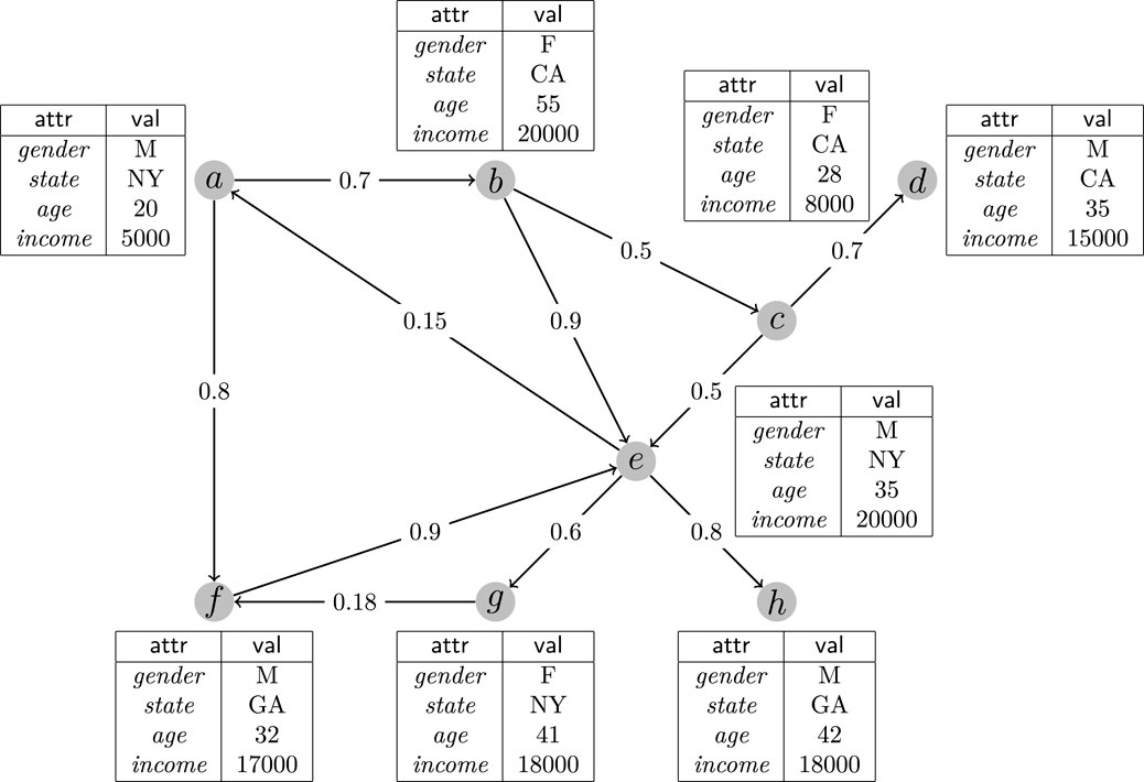
Example 1. As shown in Figure 1, there is a social network whose relationships can be represented by the graph structure. The node labelled by “a” maintains the information about a man aged 20 lived in “NY” whose salary is 5,000 per month. Also, the information associated with other nodes in the graph can be explained similarly. Each directed edge between two nodes u and v means that u can influence v. The edge between a and f is labelled by 0.8, it means that when receiving a message from a the probability that f will accept and transform the message is 0.8. That is, the value in the middle of each edge is the corresponding influence probability.
Let us consider a simple example. Suppose there is only one seed node b during the information propagation, since there is only one path between b and d, the probability that d will be influenced at last will be pb,d = 0.5 × 0.7 = 0.35. The general influence maximization problem is to find a seed node set such that after the information propagation procedure the expected number of nodes influenced is maximized.
Now, consider a case that the user want to select some nodes to help him to make an advertisement of an expensive razor. In this application, the target set may be naturally expected to be the male persons with high salary (no less than 15,000). That is, only the seed nodes with high influences to the nodes in {d, e, f, h} should be considered. Moreover, to specify the target set exactly and briefly, multi-dimensional range query is a proper choice, which can express the above requirements by a statement q: (gender = “M”) ∧ (income ≥ 15000).
As far as known by us, there are no previous works focusing on the targeted influence maximization problem based on multi-dimensional queries. To provided quick response to the targeted influence maximization problem based on multi-dimensional queries, there are at least two challenges. 1) Different from previous methods, since the target set is specified in a non-trivial way, efficient techniques for collecting the exact target set for an ad-hoc query must be developed. 2) To return the seed node set efficiently, the idea of using previously cached results should be well exploited. Although in the area of topic aware influence maximization [3] has investigated such method, it is not proper for the cases when the target set is specified by multi-dimensional queries.
Therefore, in this paper, we address the problem of Multidimensional Selection based Targeted Influence Maximization, MSTIM for short. To support efficient evaluation of queries specifying the target set, an index based solution is utilized to reuse the previous query results. While to compute the corresponding influence maximization problem efficiently, a sample based method is developed based on previous works, and it is extended to an index based solution which can reuse the samples obtained before and improve the performance significantly. The main contributions of this paper can be summarized as follows.
1. We identify the effects of multi-dimensional queries to specify the target set in the influence maximization problem, and propose the formal problem definition of Multidimensional Selection based Targeted Influence Maximization (MSTIM for short) based on a brief and expressive fragment of general multi-dimensional queries.
2. We show the computational hardness of the MSTIM problem, in fact, even if a very simple case that the target set specified is 1 larger than the seed node set, the MSTIM problem is still NP-hard.
3. Based on the Reverse Influence Sampling (RIS for short) method previously proposed, for the MSTIM problem, the basic framework of RIS is extended and shown to have a 1 − 1/e − ϵ approximation ratio when a sampling size is satisfied.
4. The index-based solution for the MSTIM problem is proposed. Using indexes of queries previously maintained, the performance of evaluating multi-dimensional queries are improved by reusing the results computed before. Sophisticated techniques for handling searching query predicates are designed and well studied. By the help of indexes of previous samples and the inverted index between nodes and samples, the MSTIM problem can be solved efficiently.
5. The experimental results on real datasets show that the proposed method is indeed rather efficient.
The rest parts of the paper are organized as follows. In section 2, some background information are introduced. Then, in section 3, the theoretical analysis of the MSTIM problem is given. Section 4 provides the basic framework of the sampling based approximation solution for the MSTIM problem. In section 5, the index version is proposed and introduced in details. Section 6 shows the experimental results. Related works are discussed in section 7, and the final part is the conclusion.
2 Related Work
The influence maximization is an important and classical problem in the research area of online social networking, which has many applications such as viral marketing, computational advertising and so on. It is firstly studied by Domingo and Richardson [4,5], and the formalized definitions and comprehensive theoretical analysis are given in [6]. Different models have been formally defined to simulate the information propagation processes with different characteristics, the two most popular models are the Independent Cascade (IC for short) and Linear Threshold (LT for short) models. In [6], the influence maximization problems under both IC and LT models are shown to be NP-hard problems and the problem of computing the exact influence of given nodes set is shown to be ♯P-hard problem in [7].
After the problem is proposed, many research efforts have been made to find the node set with maximum influence [6]. Proposed an algorithm for influence maximization based on greedy ideas which has constant approximation ratio (1 − 1/e), whose time cost is usually expensive for large networks. To overcome the shortcomings of greedy based algorithms [8], proposed CELF (Cost-Effective Lazy-Forward) algorithm, which can improve the performance of greedy based algorithms for influence maximization by reducing the times of evaluations of influence set of given seed set [9]. Proposed SIMPATH algorithm in LT model which improve the performance of greedy based influence maximization algorithm in LT model. Similar works focusing on improve the performance of influence maximization algorithms can be found also, such as [10–12] and so on. Recently, a series of sampling based influence maximization algorithms such as [13–15] are proposed and well developed, which have improved the practical performance greatly by involving a tiny loss on the approximation ratio. However, as shown by [16,17], the efficiency problem is still challenging for applying influence maximization algorithms in real applications.
The work most related with ours is [3], which focuses on the topic aware targeted influence maximization problem. In the topic aware setting, each node is associated with a list of interesting topics and the query is specified in the form of topic list. After calculating the similarities between users and the query, a weight can be assigned to the node such that the general optimizing goal of IM problem is extended to the weighted case. A sampling based solution under the help of indexes are given in [3]. Indexes are built for each keyword refereed in the topic setting. When a random query is given, the topic list associated with the query will be weighted and the computations of the similarities will be assigned to each keyword, and finally the samples are collected by combining the samples maintained for each keyword. Different from this paper, the work is not proper for the case that an exact subset of the whole network is expected to be the target set. Considering the case that the target set can be specified in an arbitrary way [1,2] studies the most general targeted influence maximization problems and provides efficient solutions. However, the general method adopted by them makes it almost impossible to provide efficient solutions using previous results with acceptable space cost. While this paper considers a more specific case that the target set can be described by a multi-dimensional query and utilizes the characteristics of those queries to develop sophisticated index based solutions. Therefore, the paper studies a variant of targeted influence maximization problem which is different from previous works.
There are also many works which try to extend the classic influence maximization methods to other application settings [18]. Studies the problem of influence maximization under location based social networks. In those networks, one node can be influenced by the other node if and only if they are neighbours according to their location informations, and [18] focus on the problem of finding k users which can affect maximum users in the location based social network [19]. Identifies the relation types during propagating the information and formally defines the problem of influence maximization by considering different types of relationships between nodes. A key idea is that given certain information which needs to be propagate the influence set of some node set can be computed more efficiently by reducing those edges belonging to some certain types [20]. Studies the problem of influence maximization under topic-aware applications. As shown by [21], the influence probabilities between users with special triangle structures are obviously higher than others. The above research efforts focus on totally different problems, compared with this paper, but their ideas on developing efficient influence maximization algorithms are helpful for us.
3 Preliminary
3.1 Classical Influence Maximization
The general description of information diffusion can be explained to be a propagating procedure of information over some special network. A network is denoted by a graph G(V, E). Given an information diffusion model M, the model will describe how the nodes influences others in network. In an instant state of the network, nodes in the network will be labelled by active or inactive. According to the model M, the inactive nodes may become active because of the existence of special active neighbours, whose rule is defined by M.
There are two classical methods to define the information propagation model, linear threshold and independent cascade model. This paper focuses on the independent cascade model (IC for short). In this model, for each edge (u, v) a probability puv is given to describe that u can activate v with probability puv. After initializing an active node set S0, in the ith step, every node will try to activate their neighbours. In detail, for each node u ∈ Si−1 and node v ∈ V \ Si−1, if (u, v) ∈ E, v will be activated once in probability puv. If v indeed becomes active, it will be added to Si and not be further considered in current step. Repeat this procedure until that no new nodes are added. Obviously, under a specific information propagation model, given an initial active set S over a network G, we can obtain a node set IS which can be activated when the propagation procedure is finished. Therefore, an expected value
Definition 1 (Influence Maximization, IM for short). Given a propagation graph G = (V, E) such that there is an associated probability puv for each edge (u, v) ∈ E, and an integer k > 0, the goal is to compute a node set S such that
3.2 Multidimentional Selection
To support multidimensional selections over social networks, it is necessary to consider an extended model of the general network for information propagation.
For each node v ∈ VG, there are m attributes
Then, we can define some basic concepts of multidimensional selection queries.
Definition 2 (1-Dimension Set). A 1-dimension set of a general attribute Ai is a set s = {v1, v2, … , vl} satisfying vj ∈ Dom(Ai) for each j between 1 and l.
Definition 3 (1-Dimension Range). A 1-dimensional range
Similarly, we can define the 1-dimension range (li, ui), (li, ui] and [li, ui), where the round bracket means that it excludes the boundary value.
Then, a 1-dimensional selection query q can be represented by (Ai, p) where p is a 1-dimension set s or a 1-dimension range
To be more general, we can define k-dimensional selection based on the definitions above.
Definition 4 (k-Dimensional Selection Query). A k-dimensional selection query Q, which defines a function V↦(0, 1), is composed of a set of k 1-dimensional query {q1, … , qk}. For each node v ∈ V, Q(v) = 1 or v ∈ Q(V) if and only if we have qi(v) = 1 for all qi (1 ≤ i ≤ k).
Here, given a k-dimensional selection query Q, let
Then, based on the concepts above, for a specific node set V, we can give a formal definition of the selection result of query Q as Q(V) = [v|v ∈ V and Q(v) = 1], which is used in an informal way before.
Example 2. Continue with Example 1, the network shown in Figure 1 can be transformed into the form shown in Figure 2, where each node in the network is associated with four attributes which are listed on the left. For each node, the corresponding values are shown on the right in the form of a table. Given a 2-dimensional query Q: [A1 = M, A2 ∈ (20, 40)], the query result Q(V) will include the nodes a, d, e, and f.
3.3 Multidimensional Selection Based Targeted Influence Maximization
Given a k-dimensional query Q representing the target users, it can be used to determine whether a node v is interested by checking whether Q(v) = 1. For a node set S ⊆ V, after a specific information propagation procedure, only the nodes activated which belong to the result of query Q are really interested by the users. Then, we can define the selection query based targeted influence as follows.
Definition 5 (Multidimensional Selection based Targeted Influence). Given a network graph G = (V, E, A), a k-dimensional query Q and a node set S ⊆ V, if the influence of S in classic influence maximization model is denoted by IS, the targeted influence based on Q can be represented by FS = IS ∩ Q(V).
Similarly, we can define the expected targeted influence
Definition 6 (Multidimensional Selection based Targeted Influence Maximization, MSTIM for short). Given a network graph G = (V, E, A), a k-dimensional query Q and an integer k, the problem is to find a subset S ⊆ V satisfying |S| ≤ k such that the expected size of
4 The Computational Complexity of MSTIM
Obviously, the general influence maximization problem is a special case of the MSTIM problem. Therefore, it can be known that the MSTIM problem is NP-hard when the query Q simply returns all nodes in V. Then, we can have the following result without detailed proofs.
Proposition 4.1. The MSTIM problem is NP-hard.
Of course, the above general case is very special and our interesting point is whether the MSTIM problem can be solved more efficiently when a practical query Q is met.
Intuitively, the definition of MSTIM is based on limiting the nodes influenced within a range defined by the query Q. An extreme case is that the result size of Q(V) is very small, and it is interested to study whether or not there exists an efficient algorithm for such cases. Obviously, when |Q(V)| ≤ k, the MSTIM problem can be solved efficiently simply by choosing the nodes in Q(V) into S, since the query result Q(V) can be solved by scanning every node v ∈ V and checking the dimensional predicates which will produce an algorithm in linear time. Then, it is meaningful to study whether such an algorithm can be extended to solve more cases for the MSTIM problem.
Next, we can prove that even for very limited but not trivial cases, it is still hard to solve the MSTIM problem efficiently.
Theorem 1. Given a network graph G = (V, E, A), a k-dimensional query Q and an integer k, the MSTIM problem is still NP-hard even for the case |Q(V)| = k + 1.
Proof. Consider an instance of the Set Cover problem, which is a well-known NP-complete problem, whose input includes a collection of subsets S1, S2, …, Sm of a ground set U = {u1, u2, … , un}. The question is whether there exist k of the subsets whose union is equal to U.
In [6], the Set Cover problem is shown to be a special case of the classical influence maximization problem, whose following results is that the classical influence maximization problem is NP-hard. While, in this paper, by the following reduction, it can be utilized to show that the MSTIM problem is NP-hard even for the case |Q(V)| = k + 1.
Given an arbitrary instance of the Set Cover problem, we first define a corresponding directed bipartite graph with n + m nodes like done in the proof of [6]. Suppose the bipartite graph constructed is G1 = (V1, E1). For each set Si, there is a corresponding node vi, and there is a node
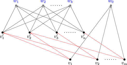
FIGURE 3. An example of the reduction, where the edge with activation probability 1 is in red and the other edges have probability c.
The following facts are essential for verifying the correctness of the reduction above.
• For the query Q, we have |Q(V)| = k + 1, and we can obtain an easy lower bound by selecting arbitrary k nodes from {w0, … , wk}. Observing that there are no output edges of the nodes in (w0, … , wk), such a method can produce a seeding node set with expected influence k exactly.
• Obviously, S should not choose nodes in
• Suppose S contains nodes in both (wi) and (vj) and there exists a set cover (St) of size k, we can always increase the influence by utilizing nodes in (vj) to replace nodes in (wi). Assume that there are x nodes of {vj} and y > 0 nodes of {wi} in S, and the x nodes can cover n − 1 nodes in
Let S′ be the nodes of {vi} corresponding to the cover {St}.
Then, we have the following results.
Obviously, we have
Then, according to the facts above, it is easy to check that there exists a solution of the set cover problem if and only if we can find k seeding nodes such that the influence obtained is at least k + 1 − k(1 − c)n − (1 − c)k.
Finally, the MSTIM problem is NP-hard even for the case |Q(V)| = k + 1.
5 The Basic Sampling Algorithm for MSTIM
5.1 Reverse Influence Sampling
RIS (Reverse Influence Sampling) based methods are the state-of-the-art techniques for approximately solving influence maximization problem. In this part, we introduce this kind of methods first. First, we introduce the concept of Reverse Reachable (RR) Set and Random RR Set.
Definition 7 (Reverse Reachable Set, [22]). Let v be a node in G, and
Definition 8 (Random RR Set, [22]). Let
Based on the two definitions above, a typical RIS based method can be described as follows.
• Generate multiple random RR sets based on G.
• Utilize the greedy based algorithm for max-coverage problem shown in [23] to find a node set A satisfying |A| ≤ k such that as many random RR sets can be covered by A as possible. The solution is a (1 − 1/e)-approximation result.
Obviously, since the second step is just a standard method for solving maximum coverage problem, to guarantee the (1 − 1/e) approximation ratio, enough samples should be gathered in the first round of the algorithm. As shown in [24], there have been several research works providing such sampling based influence maximization algorithm with 1 − 1/e − ϵ approximation ratio within time cost
Here, assuming that the sample size is presented by θ, a result shown in [22] is utilized to explain the principles of our method. Since there have been always research efforts focusing on improving the sampling size, it is easy to check that the improved version can be easily applied to the method proposed by us.
Theorem 2 [22]. If θ is at least
5.2 RIS Based Algorithm for MSTIM
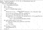
As shown in Figure 1, a conceptual algorithm is given to solve the MSTIM problem. Compared with the original version of RIS method, the random RR set is not generated by starting from an arbitrary node in G, but from a node in Q(V), where Q(V) is the nodes in the selection result of query Q.
Algorithm 1 RIS-MSTIM.
Obviously, the verify the correctness of the above algorithm, it is only needed to show that the random RR set obtained is a proper estimator of
Theorem 3. Given a set S ⊆ V, for a random RR set e of Q(V), we have
Proof. According to the definition of
Since the starting node v of Q(V) is randomly selected, for each of them the probability of being selected is
Then, similar with the analysis in [22], it can be shown that when
6 Index-Based Solution for MSTIM
6.1 Indexing for the Range Query
Since the query Q required is holistic, the result Q(V) cannot be predicated well. For the step 2 of the conceptual level algorithm RIS-MSTIM, the query result T = Q(V) is extracted to help the following sampling steps, however, evaluating the query Q may be an expensive procedure because of the multi-selection predicates [25].
A possible solution is to utilize sophisticated index to improve the query performance, such as R-Tree [26], k-d Tree [27] and so on. However, the above indexes will cause large storage overhead and usually the selection time cost using the index will increase as storage cost increases, especially when the data distribution is seriously skewed. For the worst cases, even the scanning method may become more time and space efficient [28].
Since the evaluation of the range queries is a preprocess of the whole RIS-MSTIM algorithm and most space cost will be expected to be improve the sampling performance as shown by the follows, inspired by the method used by [28], an adaptive indexing method for the range queries are utilized here to improve the performance of evaluating range queries.
There are mainly two index structures, resultPool and queryPool, utilized to improve the performance of the range query evaluation.
6.1.1 The ResultPool Index Structure
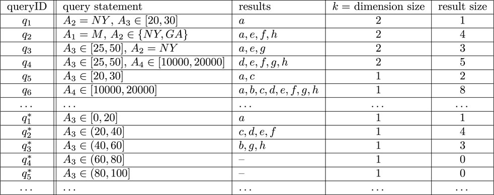
The resultPool index maintains the information about the query results of the queries processed previously, whose function is to provide a physical cache for the results such that the queries selecting a subset of some previous query can be processed efficiently. Assuming that each query can be identified by an unique queryID, as shown in Figure 4, for each qi, four parts of information are maintained in resultPool.
a) The query statement is the formal representation of the query qi.
b) The query results are the IDs of the nodes in V which belong to the set qi(V), and the nodes are listed in the ascending order of their IDs. Furthermore, the node set V can be stored in an array indexed by the nodeIDs, such that the attribute values of some node v can be accessed in constant time cost using the ID of v.
c) The dimension size k represents how many predicates are utilized in qi.
d) The result size is the size of qi(V).
The queries stored in
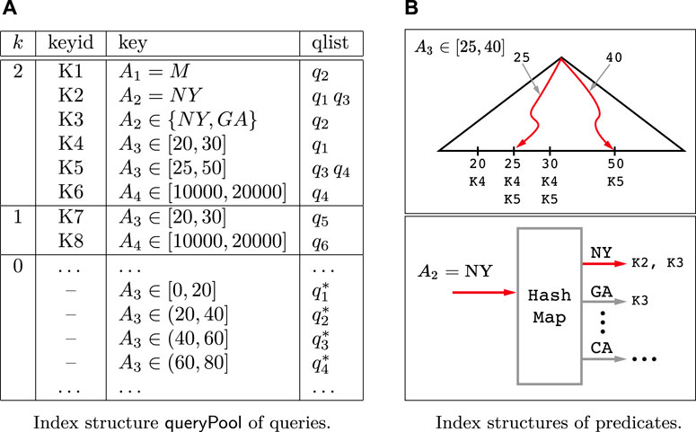
Example 3. Continue with Example 2, given the graph shown in Figure 2, as shown in Figure 4, the index structure related with a special query history {q1, q2, … } contains two parts, qis and
6.1.2 The QueryPool Index Structure
Algorithm 2 IndexOperations.
The
Given two range queries q1 and q2, q1 is contained by q2, denoted by q1 ⊆ q2, if for every data instance D there is q1(D) ⊆ q2(D). Specially, if q1 ⊆ q2 and q2 is a 1-dimensional range query, a.k.a. a predicate, we say q2 covers q1. For a set of queries {q1, … , qn}, if there is qi ⊆ qj (i ≠ j), qj is called to be a redundant one in the following.
The
Example 4. Continue with Example 3, the corresponding
6.1.3 The SearchQueryPool Procedure
Next, the principles of using the two index structures to improve the performance of range query evaluation are introduced.
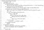
The SearchQueryPool function is shown in Algorithm 2, which will return a query Q′ for given a query Q such that the result Q(V) can be obtained efficiently based on Q′(V). First, a set candidate is initialized to be empty (line 2), which will be used to store the candidates of Q′. Then, an iteration from the group with k = |Q| to the one with k = 1 is done to generate the queries in candidate (line 3–21). For each fixed i ∈ [1, |Q|], a merge-style method is used to extract the queries containing Q efficiently by the following steps. (a) The keys covering some predicate of Q are collected, and a pointer is initialized at the front of the corresponding qlist for each key found (line 4–7). The details of obtaining keys covering some predicate will be introduced later. (b) Using the pointers initialized above, the merge-style method works by counting the appearing times of the current smallest queryID and inserting the query appearing no less than i times to the candidate set (line 8–19). At the end of each iteration, if the candidate is not empty, the iterations will stop. Finally, after the iterations, if the candidate set is not empty, an arbitrary non-redundant query in candidate is returned (line 22–24). Otherwise,
As shown in Figure 5B, to efficiently search the keys covering some predicate, for the numerical attribute we can use a tree based search structure to achieve a O(log n) time cost for search operation where n is the number of distinct values appearing in the query predicates, and for the category values a hash table can be utilized to achieve an expected O(1) time cost.
• For each numerical attribute A, a standard binary search tree is built. The search keys are chosen from the set of all distinct values appearing in the queries. In each leaf node with search key m, the keyID of each predicate qA over A satisfying m ∈ qA is stored. For example, as shown in Figure 5B, the leaf node with search key 25 includes K4 and K5 whose corresponding predicates in the
• For each category attribute A, a standard hash map is built by using the values as the hashing keys. Similarly, each item x obtained by the hash map is associated the keyIDs of the predicates in the form A = x. For example, as shown in Figure 5B, the hashed item of “NY” is associated with K2 and K3, which are keyIDs of predicates A2 = NY and A2 ∈ {NY, GA}.
Example 5. Continue with Example 4, given a query Q: (A2 = NY) ∧ (25 ≤ A3 ≤ 40), the candidate queries which contain Q can be found as follows. First, Q can be divided into two predicates q1: A3 ∈ [25, 40] and q2: A2 = NY. Then, for the group of keys with k = 2 in the
Here, the underline indicates the position of the related pointer for each list. During the merge procedure, the query q3 will be inserted into the candidate set, since in the third step q3 appears at the front of two lists. To verify the correctness, it can be found that the statement of q3 is (A3 ∈ [25, 50]) ∧ (A2 = NY) and obviously we have Q ⊆ q3.
6.1.4 Index Based Range Query Evaluation
Algorithm 3 IndexRQE (Index Based Range Query Evaluation).
Now, we will show how to obtain the exact result of a given query based on the techniques shown above. As shown in Algorithm 3, given a k − dimensional query Q, the function SearchQueryPool is first invoked to search a candidate query set q whose item will contain the query Q (line 2). The structure qres is utilized to maintain a superset of Q(V) and initialized to be empty (line 3). If q is not
Example 6. Continue with Example 5, suppose the query Q′: A3 ∈ [10, 40] is given. Obviously, there are no predicates covering Q′, therefore, the function SearchQueryPool(Q′) will return
6.2 Indexing for the Random RR Sets
6.2.1 The Indexing Structures
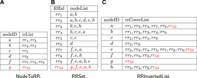
To maintain the related information of random RR sets, three index structures are utilized,
In the
Example 7. As shown in Figure 6B, a set of samples are listed in the
6.2.2 Adaptive Sampling Using Index
Algorithm 4 AdaptiveSampling.
In this part, we will explain how to sample the random RR sets adaptively under the help of indexes introduced above. As shown in Algorithm 4, the inputs of AdaptiveSampling include the network graph G, a target node set T and a sampling size θ, and the output R is a sample set of random RR sets. For each node v ∈ T, a variable cntv will be used to record the number of samples needed starting from v and initialized to be 0 (line 3–4). Then, θ nodes are randomly selected from T with replacement, different from the commonly used sampling methods this step does not start the random walking but just increases the counter variable cntv to remember that one sample is needed (line 5–7). After that, we will know the number of samples needed for each node, all left we need to do is to reuse the samples maintained in
Example 8. Let us consider the case that cntg and cntf are assigned to be 1 and 2, respectively, when running AdaptiveSampling. As shown in Figure 6, the information shown in black is the index structures before invoking AdaptiveSampling. Since cntg = 1 and there are no items with nodeID = g, one random walking will be made to obtain a new sample rr10. Then, the parts in Figure 6 shown in red will be added. For the node f, since cntf = 2 and there are three RRids in the rrList of the item with nodeID = f in
6.3 RIS-MSTIM-Index Algorithm
Finally, we introduce the main procedure of index based solution for the MSTIM problem. As shown in Algorithm 5, the RIS-MSTIM-Index function is the index version of Algorithm 1. Different from Algorithm 1, RIS-MSTIM-Index utilizes the IndexRQE method to collect the results of Q(V) (line 1). Then, during the sampling procedure, AdaptiveSampling is invoked to obtain the sample set with enough random RR sets (line 4). After that, to utilize the
Algorithm 5 RIS-MSTIM-Index.
7 Experimental Evaluation
In this part, experiments on real datasets are conducted to evaluate the efficiency and performance of the targeted influence maximization algorithm defined based on multidimensional queries.
7.1 Experiment Setup
We ran our experiments on four real datasets, Google, Youtube, Twitter, and WikiVote, which are collected from Konect (http://konect.uni-koblenz.de/) and SNAP (http://snap.stanford.edu/data/) respectively. All of them are social network datasets. Typically, the characteristic information of the four datasets are shown in Table 1. In these four social networks, nodes represent users and edges represent friendships between users. All experiments were executed on a PC with 3.40 GHz Intel Core i7 CPU and 32 GB of DDR3 RAM, running Ubuntu 20.04.
We compare two versions of the influence maximization algorithm proposed. For RIS algorithm, it means that the baseline method shown in Algorithm 1, where a trivial method is utilized to obtain the query result first and the commonly used RIS method is utilized to solve the corresponding targeted influence maximization problem. While, for RIS-MSTIM-Index algorithm, it means that the index version of Algorithm 1, which utilizes the
For each dataset, the dimensions and values of the nodes are generated randomly. For each node, 5 category dimensions and 10 numerical dimension are associated and the corresponding values are randomly selected in an uniform way within the value domain. To evaluate the query based targeted influence maximization algorithm, multidimensional range queries are generated in the following way. For each dataset, 10 group of queries are generated randomly, within each group, there are 50 queries in total. The dimension number of each query is chosen between 1 and 5 according to a normal distribution, most of the queries have three or four predicates. A query is only allowed to contain at most one predicate on each dimension. The range predicates are also randomly generated by controlling the selectivities to be about 20%. Usually, to be simple, we use the number of queries and random RR sets to control the index size. It should be remarked that the controlling method is not an accurate way since the size of each query or sample is not known, but it can avoid complex calculating the index size which may affect the performance of the main algorithm.
7.2 Experimental Results and Analysis
The experimental results are conducted to verify the efficiencies of the influence maximization algorithm proposed from several aspects.
7.2.1 Efficiency of RIS-MSTIM Algorithm
To study the efficiencies of the RIS-MSTIM algorithm proposed, for each real dataset, both the RIS-MSTIM algorithms with and without indexes are executed to solve the targeted influence maximization problem. To measure the performance of RIS-MSTIM fairly when considering different queries, 10 range query groups, each of which contain 50 queries, are generated randomly. For each group of queries, RIS-MSTIM algorithm is invoked to solve the corresponding targeted influence maximization problem. Within each group, the performance of RIS-MSTIM will become better as the increase of the number of queries processed, assuming that there are enough space costs to maintain the corresponding indexes. For each same setting, the algorithm is ran 5 times and the average time costs are recorded.
As shown in Figure 7, executing the RIS-MSTIM algorithms with and without indexes over the four datasets, when the seed size k is increased from 5 to 80, the average time costs for evaluating each group of queries generated are reported. Here, for the previous three datasets, the average time cost of 10 group of queries are reported, while for the youtube dataset the average time cost of 3 group of queries are reported since it will take much longer time than other datasets. Based on the above results, we have two observations. The first one is that as the seed size increases in an exponential speed both the index and no-index versions of RIS-MSTIM can scale well, where it should be noted that the seed size is enlarged twice each time. The second one is that using the indexes the RIS-MSTIM algorithm performances much better, where the indexes can help the reduce the time costs to about 50% for all datasets. It is verified that the index based idea of improving the performance of RIS-MSTIM is effective and can be utilized in rather diverse settings for which within the experiments there are about 500 queries and five different seed sizes. Moreover, since the datasets used here have different characteristics, it has been also verified that our index based method is proper for different types of data.
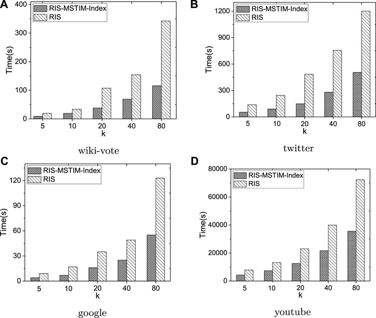
FIGURE 7. The average time cost of targeted influence maximization algorithm for evaluating the randomly generated query groups over four datasets.
Also, it is verified that the index based solution can be applied to other sophisticated method within RIS framework also. As shown in Figure 8, using BCT method in [1] which is the state of the art and the same setting, for wiki-vote and google datasets, the average time costs of BCT methods with and without index are compared. It can be observed that the index solution proposed by this paper can improve the performance of BCT based method significantly also. The second key observation is that, although BCT is better than the standard RIS method, the total time costs caused by BCT and RIS methods are nearly same. The reason is that the cost of performing targeted influence maximization is highly dominated by the cost of evaluating multi-dimensional queries.

FIGURE 8. The average time cost of BCT based targeted influence maximization algorithm for evaluating the randomly generated query groups over two datasets.
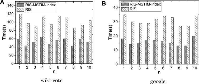
As shown in Figure 9, fixing the seed size to be 20, the time costs for evaluating each query group are reported. In Figure 9A, over the wiki-vote dataset, the results for 10 groups of queries are shown, where as discussed above each of the group contains 50 queries and the label n of x-axis means the group id. Similarly, the experimental results over google dataset is shown in Figure 9B. It can be observed that over those two datasets the performance of RIS-MSTIM method can be improved by using indexes for all the query group randomly generated.
7.2.2 Effectiveness of Adjusting Index Sizes
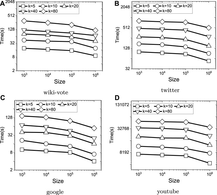
To evaluate the effects of index sizes, the memory size used by the indexes are controlled by limiting the total number of queries and random RR sets cached by the indexes. The total size is changed between 1 and 1000 K, where each time it is increased by 10 times. For each dataset, the average time costs of evaluating the targeted influence maximization algorithm for the 10 groups of queries generated are recorded. As shown in Figure 10, when increasing the index size, the time costs over all four datasets are reduced. Since increasing the index size can enlarge the probability that a random chosen query share random RR sets with previous queries, such an observation is just what are expected. Therefore, it can be verified that the indexes using by the algorithm is the essential part for improving the performance of RIS-MSTIM, and when being allowed, the threshold for controlling index size should be assigned to a value as large as possible.
7.2.3 The Space Cost of Indexes
Intuitively, to let the index based method more general and usable, the space cost of the indexes used should be well controlled. Intuitively, when it is assumed that the memory is enough large to contain all possible index items, without considering the maintaining and searching costs of the indexes, the performance of the influence maximization algorithms can only become better when more items are indexed. Although, the maintaining and searching costs are relatively small comparing with the total time cost of RIS-MSTIM, it still needs huge space cost to store the sampled random RR sets temporally. If the indexes consume too many space costs, there may be only few space to store the new samples needed and the algorithm will perform very bad because of no enough memory space. In this part, fixing the index control size as 1000 K, for the four datasets, we run RIS-MSTIM algorithm over them for the parameter settings k ∈ {5, 10, 20, 40, 80}. Then, the sizes of indexes for query results and random RR sets are reported. As shown in Table 2, the space cost of RIS-MSTIM with index over the youtube dataset is the largest and the cost over the wiki-vote dataset is the smallest, which is expected based on the observation about the execution time costs. Generally speaking, when the seed size becomes larger, the space cost increases also. For the google and wiki-vote datasets, when the seed size is rather smaller, because that the space cost of all samples generated is still smaller than the threshold, the cost labelled by
7.2.4 Comparison of Influence Obtained
Since the two versions of the RIS-MSTIM algorithm are the same one in principle, the effects of solving targeted influence maximization problem should be the same also. However, the key idea utilized in the index version is to reuse the samples obtained before, therefore, the detailed execution of the two RIS-MSTIM algorithms may be different. In this part, we should verify that the difference discussed above is very tiny such that we can ignore them when considering the qualities of the solutions obtained.
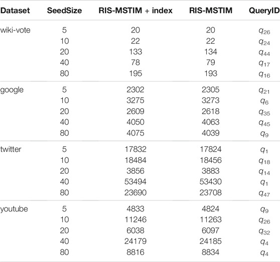
Since for each parameter setting, 50 queries in total are ran, we randomly select one query for each setting, record the seed node set, evaluate and compare their corresponding influence obtained. The results are shown in Table 3. It can be observed that there are tiny differences between the influence values obtained by RIS-MSTIM with and without indexes. This is as expected since the algorithm is a randomized one which only makes sure that a (1 − 1/e − ϵ) approximation solution is obtained with at least (1 − δ) probability. Also, it can be observed that the differences are acceptable for each dataset when considering the total dataset sizes.
8 Conclusion
In this paper, the problem of multidimensional selection based Targeted Influence Maximization is studied. The MSTIM problem is shown to be NP-hard even when the target set is rather small. The RIS framework is extended to the MSTIM case, based on a careful analysis of the sampling size, it is shown that the MSTIM problem admits a 1 − 1/e − ϵ approximation algorithm based on reverse influence sampling. To answer the MSTIM problem efficiently, an index based solution is proposed. To improve the performance of evaluating multi-selection queries, an inverted list style index for query predicates is presented, and efficient index based query evaluation method is developed. To improve the performance of the sampling procedure, using the idea of sharing samples as much as possible, an adaptive sampling strategy based on index is introduced and the corresponding influence maximization algorithm is designed. The experimental results show that the method proposed is efficient.
Data Availability Statement
Publicly available datasets were analyzed in this study. This data can be found here: http://snap.stanford.edu/data/ http://konect.uni-koblenz.de/.
Author Contributions
DJ completes the main work and updates the manuscript of this paper. TL gave the main idea of the key method, designed the study, and helped to draft the manuscript. All authors read and approved the final manuscript.
Funding
This work is supported by the National Key Research and Development Program of China (2018AAA0101901), the National Natural Science Foundation of China (NSFC) via Grant 61976073 and 61702137.
Conflict of Interest
The authors declare that the research was conducted in the absence of any commercial or financial relationships that could be construed as a potential conflict of interest.
Publisher’s Note
All claims expressed in this article are solely those of the authors and do not necessarily represent those of their affiliated organizations, or those of the publisher, the editors and the reviewers. Any product that may be evaluated in this article, or claim that may be made by its manufacturer, is not guaranteed or endorsed by the publisher.
References
1. Nguyen HT, Thai MT, Dinh TN. A Billion-Scale Approximation Algorithm for Maximizing Benefit in Viral Marketing. Ieee/acm Trans Networking (2017) 25:2419–29. doi:10.1109/tnet.2017.2691544
2. Epasto A, Mahmoody A, Upfal E. Real-time Targeted-Influence Queries over Large Graphs. In: Proceedings of the 2017 IEEE/ACM International Conference on Advances in Social Networks Analysis and Mining 2017; July 31 - August 03, 2017; Sydney, Australia (2017). p. 224–31. doi:10.1145/3110025.3110105
3. Li Y, Zhang D, Tan K-L. Real-time Targeted Influence Maximization for Online Advertisements. Proc VLDB Endow (2015) 8:1070–81. doi:10.14778/2794367.2794376
4. Domingos P, Richardson M. Mining the Network Value of Customers. In: KDD ’01 (2001). p. 57–66. doi:10.1145/502512.502525
5. Richardson M, Domingos P. Mining Knowledge-Sharing Sites for Viral Marketing. In: Proceedings of the Eighth ACM SIGKDD International Conference on Knowledge Discovery and Data Mining; New York, USA: ACM (2002). p. 61–70. KDD ’02. doi:10.1145/775047.775057
6. Kempe D, Kleinberg J, Tardos E. Maximizing the Spread of Influence through a Social Network. In: Proceedings of the Ninth ACM SIGKDD International Conference on Knowledge Discovery and Data Mining; New York, USA: ACM (2003). p. 137–46. KDD ’03. doi:10.1145/956750.956769
7. Chen W, Wang C, Wang Y. Scalable Influence Maximization for Prevalent Viral Marketing in Large-Scale Social Networks. In: KDD ’10; New York, USA: ACM (2010). p. 1029–38. doi:10.1145/1835804.1835934
8. Leskovec J, Krause A, Guestrin C, Faloutsos C, VanBriesen J, Glance N. Cost-effective Outbreak Detection in Networks. In: Proceedings of the 13th ACM SIGKDD International Conference on Knowledge Discovery and Data Mining; New York, USA: ACM (2007). p. 420–9. KDD ’07. doi:10.1145/1281192.1281239
9. Goyal A, Lu W, Lakshmanan LVS. Simpath: An Efficient Algorithm for Influence Maximization under the Linear Threshold Model. In: ICDM ’11; Washington, DC, USA, (2011). p. 211–20.
10. Chen W, Wang Y, Yang S. Efficient Influence Maximization in Social Networks. In: Proceedings of the 15th ACM SIGKDD International Conference on Knowledge Discovery and Data Mining; New York, USA: ACM (2009). p. 199–208. KDD ’09. doi:10.1145/1557019.1557047
11. Chen Y-C, Peng W-C, Lee S-Y. Efficient Algorithms for Influence Maximization in Social Networks. Knowl Inf Syst (2012) 33:577–601. doi:10.1007/s10115-012-0540-7
12. Jiang Q, Song G, Cong G, Wang Y, Si W, Xie K. Simulated Annealing Based Influence Maximization in Social Networks. In: Proceedings of the Twenty-Fifth AAAI Conference on Artificial Intelligence. Palo Alto, CA: AAAI Press (2011). p. 127–32. AAAI’11.
13. Tang Y, Shi Y, Xiao X. Influence Maximization in Near-Linear Time. In: TK Sellis, SB Davidson, and ZG Ives, editors. Proceedings of the 2015 ACM SIGMOD International Conference on Management of Data, Melbourne; May 31 - June 4, 2015; New York, USA: ACM (2015). p. 1539–54. doi:10.1145/2723372.2723734
14. Huang K, Wang S, Bevilacqua G, Xiao X, Lakshmanan LVS. Revisiting the Stop-And-Stare Algorithms for Influence Maximization. Proc VLDB Endow (2017) 10:913–24. doi:10.14778/3099622.3099623
15. Huang K, Tang J, Han K, Xiao X, Chen W, Sun A, et al. Efficient Approximation Algorithms for Adaptive Influence Maximization. VLDB J (2020) 29:1385–406. doi:10.1007/s00778-020-00615-8
16. Arora A, Galhotra S, Ranu S. Influence Maximization Revisited: The State of the Art and the Gaps that Remain. In: M Herschel, H Galhardas, B Reinwald, I Fundulaki, C Binnig, and Z Kaoudi, editors. Advances in Database Technology - 22nd International Conference on Extending Database Technology, EDBT 2019; March 26-29, 2019; Lisbon, Portugal. Konstanz, Germany: OpenProceedings.org (2019). p. 440–3. doi:10.5441/002/edbt.2019.40
17. Arora A, Galhotra S, Ranu S. Debunking the Myths of Influence Maximization. In: S Salihoglu, W Zhou, R Chirkova, J Yang, and D Suciu, editors. Proceedings of the 2017 ACM International Conference on Management of Data, SIGMOD Conference 2017; May 14-19, 2017; New York, USA: ACM (2017). p. 651–66. doi:10.1145/3035918.3035924
18. Li G, Chen S, Feng J, Tan K, Li W. Efficient Location-Aware Influence Maximization. In: Proceedings of the 2014 ACM SIGMOD International Conference on Management of Data; New York, USA: ACM (2014). p. 87–98. SIGMOD ’14. doi:10.1145/2588555.2588561
19. Tang S, Yuan J, Mao X, Li X, Chen W, Dai G. Relationship Classification in Large Scale Online Social Networks and its Impact on Information Propagation. In: INFOCOM 2011 (2011). p. 2291–9. doi:10.1109/infcom.2011.5935046
20. Chen S, Fan J, Li G, Feng J, Tan K-l., Tang J. Online Topic-Aware Influence Maximization. Proc VLDB Endow (2015) 8:666–77. doi:10.14778/2735703.2735706
21. Zhang J, Tang J, Zhong Y, Mo Y, Li J, Song G, et al. Structinf: Mining Structural Influence from Social Streams. In: AAAI’17 (2017). p. 73–80.
22. Tang Y, Xiao X, Shi Y. Influence Maximization: Near-Optimal Time Complexity Meets Practical Efficiency. In: SIGMOD 2014 (2014). p. 75–86.
23. Khuller S, Moss A, Naor J. The Budgeted Maximum Coverage Problem. Inf Process Lett (1999) 70:39–45. doi:10.1016/s0020-0190(99)00031-9
24. Li Y, Fan J, Wang Y, Tan K-L. Influence Maximization on Social Graphs: A Survey. IEEE Trans Knowl Data Eng (2018) 30:1852–72. doi:10.1109/tkde.2018.2807843
25. Gaede V, Günther O. Multidimensional Access Methods. ACM Comput Surv (1998) 30:170–231. doi:10.1145/280277.280279
26. Guttman A. R-trees: A Dynamic index Structure for Spatial Searching. In: SIGMOD’84, Proceedings of Annual Meeting; June 18-21, 1984. Boston, Massachusetts, USA (1984). p. 47–57.
27. Bentley JL. Multidimensional Binary Search Trees Used for Associative Searching. Commun ACM (1975) 18:509–17. doi:10.1145/361002.361007
28. Lamb A, Fuller M, Varadarajan R, Tran N, Vandiver B, Doshi L, et al. The Vertica Analytic Database. Proc VLDB Endow (2012) 5:1790–801. doi:10.14778/2367502.2367518
29. Borgs C, Brautbar M, Chayes J, Lucier B. Maximizing Social Influence in Nearly Optimal Time. In: Proceedings of the Twenty-Fifth Annual ACM-SIAM Symposium on Discrete Algorithms; USA: Society for Industrial and Applied Mathematics. Philadelphia, PA. SODA ’14 (2014). p. 946–57. doi:10.1137/1.9781611973402.70
Keywords: targeted, influence maximization, index, sampling, multidimensional selection
Citation: Jing D and Liu T (2021) Efficient Targeted Influence Maximization Based on Multidimensional Selection in Social Networks. Front. Phys. 9:768181. doi: 10.3389/fphy.2021.768181
Received: 31 August 2021; Accepted: 09 November 2021;
Published: 06 December 2021.
Edited by:
Chengyi Xia, Tianjin University of Technology, ChinaReviewed by:
Peican Zhu, Northwestern Polytechnical University, ChinaZhen Wang, Hangzhou Dianzi University, China
Copyright © 2021 Jing and Liu. This is an open-access article distributed under the terms of the Creative Commons Attribution License (CC BY). The use, distribution or reproduction in other forums is permitted, provided the original author(s) and the copyright owner(s) are credited and that the original publication in this journal is cited, in accordance with accepted academic practice. No use, distribution or reproduction is permitted which does not comply with these terms.
*Correspondence: Ting Liu, dGxpdUBpci5oaXQuZWR1LmNu
 Dong Jing
 Ting Liu*