Department of Physics, NIT Sikkim, South Sikkim, India
Investors adopt varied investment strategies depending on the time scales (τ) of short-term and long-term investment time horizons (ITH). The nature of the market is very different in various investment τ. Empirical mode decomposition (EMD) based Hurst exponents (H) and normalized variance (NV) techniques have been applied to identify the τ and characteristics of the market in different time horizons. The values of H and NV have been estimated for the decomposed intrinsic mode functions (IMF) of the stock price. We obtained and for the IMFs with τ ranging from a few days to 3 months and 5 months, respectively. Based on the value of , two time series have been reconstructed from the : a) short-term time series [] with and τ from a few days to 3 months; b) long-term time series with and 5 months. The and show that market dynamics is random in short-term and correlated in long-term . We have also found that the is very small in the short-term ITH and gradually increases for long-term . The results further show that the stock prices are correlated with the fundamental variables of the company in the long-term . The finding may help the investors to design investment and trading strategies in both short-term and long-term investment horizons.
Introduction
The stock market is a complex dynamical system where the evolution of the dynamics depends on the participation of different types of investors or traders [1–3]. Investors/traders participate in the stock market to gain profit implementing different investment and trading strategies depending on investment time horizons (ITH) [45]. The participation of diversified investors, reaction to the information, and short-term and long-term investment approaches play crucial roles in the movement of stock prices [4].
In the stock markets, there are mainly two types of investors: short-term investors who invest for short-term gain and long-term investors who invest for long-term gain [67]. Studies show that the for short-term investors ranges from a single day to a few months, and for long-term investors, it usually ranges from a few months to several years [89]. The fund managers and foreign exchange dealers of various countries use technical analysis for the short-term and fundamental analysis for the long-term [810]. The time scales (τ) of short-term and long-term by the investors are generally chosen in an arbitrary manner based on the investment experience [810]. So the identification of τ from stock price time series using a well defined technique may be helpful for both the short-term and long-term investors.
As the market is mean reversing in short-term [9], traders fail to generate significant returns using technical analysis [11]. On the other hand, in the long-term , an investor can generate significant return or help in making decision whether to exit from that particular stock to avoid loss by determining the financial health of a company by using fundamental variables [12–14]. Fundamental analysis is an essential tool to find out the relation between stock price and fundamental variables such as book to market (B/M), sales to price, debt to equity, earnings to price, and cash flow of a stock [12–14]. The stock price is found to be positively correlated with the essential fundamental variables [14–20]. The study of the correlation in the short-term and long-term is essential to take a fruitful investment decision.
In the short-term , the market is generally considered to be governed by psychological behavior of the investors. However, the fundamental variables are the main determining crucial factors in the long-term . Usually, investors choose the τ of short-term and long-term investment horizon in an arbitrary manner [98]. Recently, we used structural break study to show that the τ for the short-term is usually less than a few months [9]. The separation of the short- and long-term dynamics in terms of τ plays a vital role in the prediction of future price movement. Hence, detailed studies are required to find the correlation of the stock price with fundamental variables and to identify the τ of market dynamics in the short-term and long-term .
In this article, we estimated the τ of the stock price in the short-term and long-term for twelve leading global stock indices and the stock price of some companies using empirical mode decomposition () based Hurst exponent (H) analysis. We have reconstructed short-term and long-term time series based on the H. Finally, we estimated the correlation coefficient between long-term time series and fundamental variables. Herein we establish that short-term is normally less than 3 months and long-term is more than 5 months. Correlation analysis shows that the long-term stock price is positively correlated with the fundamental variables.
The remaining part of this paper is organized as follows: In Section 2, we introduce the method of analysis, while Section 3 presents the data analyzed. Results and discussion and conclusion are delineated in Sections 4 and 5, respectively.
Method of Analysis
A nonlinear two-step technique—EMD followed by Hilbert–Huang Transform ()—has been applied to analyze the stock data as it is nonlinear and nonstationary. Nonlinearity in the stock market appears due to the presence of market frictions and transaction costs, existence of bid-ask spread, and short selling, whereas nonstationarity appears due to different time scales present in the stock market [2122]. This approach helps us to identify the characteristic τ and the important trends and components present in the data [3].
The method decomposes the stock index and stock price into the intrinsic oscillatory modes of different τ by preserving the nonstationarity and nonlinearity of the data. These oscillatory modes are termed intrinsic mode functions (). The can be both amplitude and frequency modulated as well as nonstationary [2324]. The τ of each has been identified by The eliminates the spurious harmonic components generated due to the nonlinearity and nonstationarity of the data [2324].
The satisfy the following two conditions; i) the number of extrema and the number of zero crossing must be equal or differ by one; and ) mean values of the envelope, defined by the local maxima and local minima, for each point are zero. The is calculated in the following way [2325]:
a. Lower envelope and upper envelope are drawn by connecting minima and maxima of the data, respectively, using spline fitting.
b. Mean value of the envelope is subtracted from the original time series to get new data set
c. Repeat the processes (a) and (b) by considering h as a new data set until the conditions (i and ) are satisfied.
Once the conditions are satisfied, the process terminates, and h is stored as the first . The second is calculated repeating the above steps (a)–(c) from the data set . When the final residual is monotonic in nature, the steps (a)–(c) are terminated and the original time series can be written as a set of plus residue,
where represents the ith , and residue represents the trend of the stock data.
are the signal with different τ. The is a signal with the smallest τ, the is the signal with the second smallest τ, and so on. Hence, technique is useful to extract different τ from the signal. The characteristic τ of each can be estimated from the frequency (ω) by using Hilbert Transform, which is defined as
where P is the Cauchy principle value, and where , and [23]. Identification of important is essential to differentiate the market dynamics in short-term from long-term , and the differentiation can be done by evaluating the H.
Rescaled-range (R/S) analysis is a technique to estimate the correlation present in a time series by calculating H [26–28]. Details of the R/S technique are described below. Let us consider a time series of length L and divided into p subseries of length l. Each subseries is denoted as , where t = 1, 2, 3, …, p. Mean and standard deviation of the subseries are defined as
and
respectively. Mean adjusted series is calculated as
for j = 1, 2, 3, …, l. Cumulative time series is given by
for j = 1, 2, 3, …, l.
Range of the series has been calculated as
Individual subseries range can be rescaled or normalized by dividing the standard deviation. So, R/S is written as
The ratio of each subseries of length l is expressed as , where H is the Hurst exponent. H can be estimated from the slope of ln(R/S) vs. ln(l). For a random time series, H is around 0.5, and for correlated and anticorrelated time series, H is greater than 0.5 and less than 0.5, respectively.
Normalized variance () is another important statistical tool to identify the important based on the energy of the signal. The higher the value is, more significant the signal is. The technique estimates the energy of the ith by calculating variance [2930], and of ith is defined as
where q is the total number of .
Data Analyzed
We have analyzed the stock indices and stock prices of a few companies of different countries from December 1995 to July 2018, namely, 1) S&P 500 (USA), 2) Nikkei 225 (Japan), 3) CAC 40 (France), 4) IBEX 35 (Spain) 5) HSI (Hong Kong), 6) SSE (China), 7) BSE SENSEX (India), 8) IBOVESPA (Brazil), 9) BEL 20 (Euro-Next Brussels), 10) IPC (Mexico), 11) Russell 2000 (USA), and 12) TA125 (Israel), and stock prices of the companies 1) IBM (USA), 2) Microsoft (USA), 3) Tata Motors (India), 4) Reliance Communication (RCOM) (India), 5) Apple Inc. (USA), and 6) Reliance Industries Limited (RIL) (India). Stock indices and price data were downloaded from yahoo finance, and the analysis was carried out using MATLAB software.
Results and Discussions
The stock market shows different behavior in different investment horizon. based H and techniques have been applied to analyze the market dynamics as discussed below.
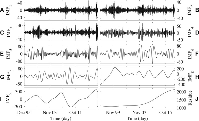
Figures 1A–J show the to and the residue of the S&P 500 index calculated using technique as described in detail in Section 2. in Figure 1A represents the mode with the lowest τ, and it gradually increases with the increase in numbers. Figure 1J represents the residue of the signal, which indicates the overall trend of the index. Similarly, we have calculated all for all the indices and companies to analyze the market.
FIGURE 1
FIGURE 1. The plots (A)–(I) represent the to , respectively, and (J) represents residue of the S&P 500 index.
Based H and Analysis
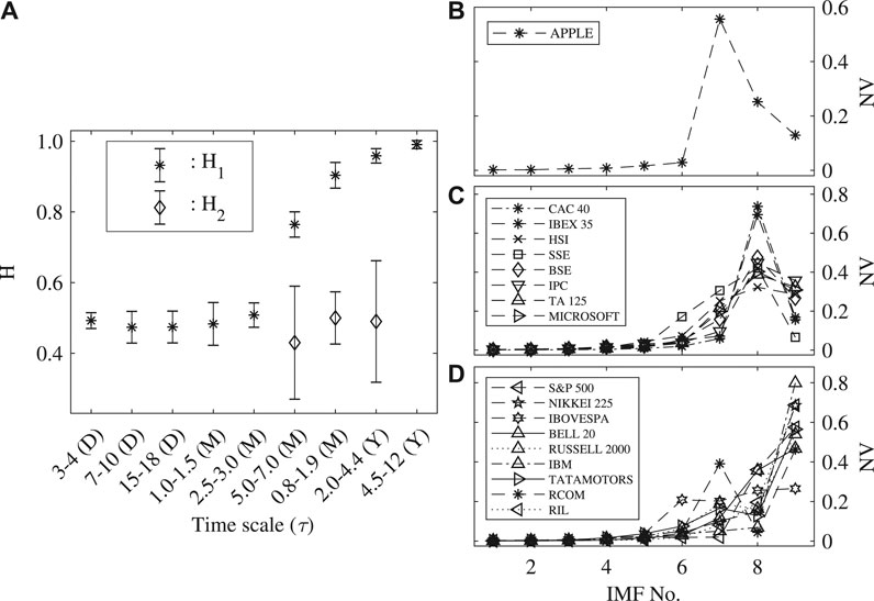
H has been calculated for all the . Figure 2A shows the typical plot of H versus τ of all the indices and companies. We obtained single H from and it is indicated as . Higher-order shows two H, namely, and . We obtained for to with τ ranging from a few days (D) to 3 months (M). The value of jumps to for with M. It gradually increases for to with a τ ranging from 1 year (Y) to 12 Y. for to indicates that the nature of the first five is random. to show a long-range correlation up to one period . τ of , , , , and of all the indices and companies stock data analyzed here are in the range of 3–4 D, 7–10 D, 15–18 D, 1–1.5 M, and 2.5–3 M, respectively.
FIGURE 2
FIGURE 2. (A) shows the Hurst exponents ( and ) vs. τ of all the of all the indices and companies with error bar. The first point represents the average value of of all the first of all stock data, the second point represents the average value of of all the second of all stock data, and so on. For to of all indices and companies with a maximum τ of around 3 M. The value of jumps to for (with a ) and gradually increases for to . value shows that nature of to is random and to have a long-range correlation. (D), (M), and (Y) in the x-axis represent the day, month, and year, respectively. (B)–(D) represent the normalized variance of s of all the indices and company, respectively.
To further validate the robustness of the proposed method, analysis of the decomposed time series has been carried out using technique. Figures 2B–D represent of all the of all the indices and companies, where plots have been arranged according to the order of higher of . Figures 2B–D show that the value of is very low for all the indices and companies up to , and increases significantly for to . Hence, based on the value of the time series can also be decomposed into two time series with two distinct time horizons: short-term time series by adding to and long-term time series by adding to plus residue as described in Section 4.2. Further, technique can be used to find a time series with important time scale in the form of Figures 2B–D show that the value of is higher for with , with , and with , respectively, for the companies mentioned in the plots. The decomposed time series with higher value of may play important role to predict long-term behavior of the market [29]. More such studies in detail can be pursued in future.
Reconstruction of Short-Term and Long-Term Time Series
In order to analyze the market dynamics in short-term and long-term , we have reconstructed two time series from the decomposed as discussed below.
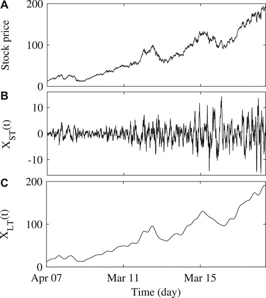
We have reconstructed a time series by adding the to whose , that is, . The time scale of ranges in . Figure 3B shows the reconstructed time series obtained by decomposing the original time series of Apple Inc. which is shown in Figure 3A. shows that the stock market is random when τ ranging from a few days to 3 months. Hence, represents the short-term time series in . The above analysis shows that the market behavior is random in the short-term when τ is in the range of a few days to 3 months.
FIGURE 3
FIGURE 3. (A) represents the daily price movement of Apple Inc. from April 2007 to March 2018. (B),(C) represent the reconstructed short-term time series and long-term time series , respectively.
Higher-order shows two Hurst exponents ( and ). We have reconstructed another time series by adding to whose and residue, that is, residue to understand the market dynamics in long-term . The time scales of are . Figure 3C shows the reconstructed long-term time series obtained by decomposing the original time series of Apple Inc., which is shown in Figure 3A. The present analysis yielded a value of , which shows that the stock market has a long-range correlation with . Hence, represents the long-term time series with . From the above analysis, it can be concluded that the market has a long-range correlation in the long-term with and hence may be used to predict a future price. Further, it has been observed that the future price of a stock is actually much more dependent on the fundamental variables of a company. In order to understand such dependence, we have studied the correlation between and the fundamental variables of the companies.
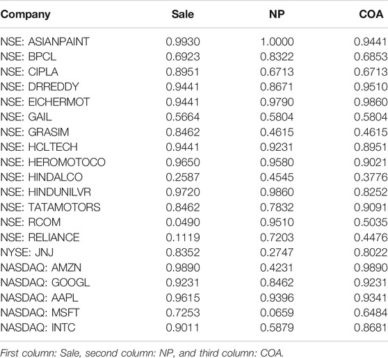
Table 1 shows that the correlation coefficient (J) between and three fundamental variables: sale, net profit (NP), and cash from operating activity (COA) for some Indian and American companies which are listed in NSE, NYSE, and NASDAQ, from March 2007 to March 2018 in the annual price level. Fundamental variables data have been downloaded from screener and macrotrends. We obtained a positive correlation between and sale, NP, and COA for all the years. It implies that stock price is correlated with the sale, NP, and COA. We have obtained a small J for a few stocks. These stocks show a small J for the following two possible reasons: a) the stock price of a company with strong growth prospect increases even though sale or NP decreases temporarily; b) the stock price of a company with weak growth prospect decreases even though sale or NP increases temporarily. Hence, for long-term investment, the fundamental variables are the most crucial variables for the prediction of the future price. In the future, we would like to study the correlation between stock price and other fundamental variables of companies.
TABLE 1
TABLE 1. Correlation coefficient between reconstructed long-term time series and three fundamental variables of some Indian and American companies.
Conclusion
In this paper, we have studied the stock market using the empirical mode decomposition () based Hurst exponent (H) analysis and normalized variance () technique. technique has been applied to decompose the time series in the form of . H and have been calculated for all the to understand the nature of the market dynamics.
The analysis yielded a value of for to . A short-term time series is reconstructed by adding to . The time scale of ranges from a few days to 3 months. The estimated value of which shows that the stock market is random in the short-term . We have estimated the value of , , , and for , , , and , respectively, for all the data. shows that the to have long-range correlation, and hence a long-term time series is reconstructed by adding to and residue. The time scale of is greater than 5 months. The results show that the market is random with and having a long-range correlation with . The study of the correlation between and sale, net profit, and cash from operating activity of different companies shows that the market is positively correlated with the fundamental variables of a company in long-term . Hence, the dynamics of the market may be predicted in long-term using fundamental variables.
A detailed study of the market in the long-term in terms of fundamental variables of a company is necessary to predict the future price. We believe that the outcome of the present study may help in making investment decisions in both short-term and long-term .
All the authors have equally contributed to preparing the manuscript.
Conflict of Interest
The authors declare that the research was conducted in the absence of any commercial or financial relationships that could be construed as a potential conflict of interest.
Acknowledgments
The authors acknowledge the help of Taraknath Kundu and suggestions of the anonymous reviewers in preparing and improving the manuscript.
References
1. Mantegna RN, Stanley HE. Introduction to econophysics: correlations and complexity in finance.. Cambridge, United Kingdom: Cambridge University Press (1999).
2. Bouchaud J-P, Potters M. Theory of financial risk and derivative pricing: from statistical physics to risk management.. Cambridge, United Kingdom: Cambridge University Press (1999).
3. Huang NE, Wu M-L, Qu W, Long SR, Shen SS. Applications of Hilbert–Huang transform to non-stationary financial time series analysis. Appl Stoch Model Bus Ind (2003). 19:245–68. doi:10.1002/asmb.501
4. Peters EE, Peters ER, Peters D. Fractal market analysis: applying chaos theory to investment and economics., Vol. 24. Hoboken, NJ: John Wiley & Sons (1994).
5. Jegadeesh N, Titman S. Returns to buying winners and selling losers: implications for stock market efficiency. J Finance (1993). 48:65–91. doi:10.1111/j.1540-6261.1993.tb04702.x
8. Menkhoff L. The use of technical analysis by fund managers: international evidence. J Bank Finance (2010). 34:2573–86. doi:10.1016/j.jbankfin.2010.04.014
9. Mahata A, Bal DP, Nurujjaman M. Identification of short-term and long-term time scales in stock markets and effect of structural break. Phys Stat Mech Appl (2019). 12:123612. doi:10.1016/j.physa.2019.123612
10. Lui Y-H, Mole D. The use of fundamental and technical analyses by foreign exchange dealers: Hong Kong evidence. J Int Money Finance (1998). 17:535–45. doi:10.1016/s0261-5606(98)00011-4
12. Samaras GD, Matsatsinis NF, Zopounidis C. A multicriteria dss for stock evaluation using fundamental analysis. Eur J Oper Res (2008). 187:1380–401. doi:10.1016/j.ejor.2006.09.020
15. Basu S. Investment performance of common stocks in relation to their price-earnings ratios: a test of the efficient market hypothesis. J Finance (1977). 32, 663–82. doi:10.1111/j.1540-6261.1977.tb01979.x
21. Hasanov M. Is South Korea’s stock market efficient? Evidence from a nonlinear unit root test. Appl Econ Lett (2009). 16:163–7. doi:10.1080/13504850601018270
23. Huang NE, Shen Z, Long SR, Wu MC, Shih HH, Zheng Q, et al. The empirical mode decomposition and the hilbert spectrum for nonlinear and non-stationary time series analysis. Proc R Soc Lond A Math Phys Eng Sci (1998). 454:903–95. doi:rspa.1998.0193
24. Huang W, Shen Z, Huang NE, Fung YC. Engineering analysis of biological variables: an example of blood pressure over 1 day. Proc Natl Acad Sci USA (1998). 95:4816–21. doi:10.1073/pnas.95.9.4816
25. Chowdhury S, Deb A, Nurujjaman M, Barman C. Identification of pre-seismic anomalies of soil radon-222 signal using Hilbert–Huang transform. Nat Hazards (2017). 87:1587–606. doi:10.1007/s11069-017-2835-1
27. Nurujjaman M, Iyengar AS. Realization of SOC behavior in a dc glow discharge plasma. Phys Lett (2007). 360:717–21. doi:10.1016/j.physleta.2006.09.005
29. Chatlani N, Soraghan JJ. EMD-based filtering (EMDF) of low-frequency noise for speech enhancement. IEEE Trans Audio Speech Lang Process (2012). 20:1158–66. doi:10.1109/tasl.2011.2172428
30. Zao L, Coelho R, Flandrin P. Speech enhancement with emd and hurst-based mode selection. IEEE/ACM Trans Audio Speech Lang Process (2014). 22:899–911. doi:10.1109/taslp.2014.2312541
Keywords: empirical mode decomposition, Hurst exponent, short-term investment time horizon, long-term investment time horizon, time scale, normalized variance
Citation: Mahata A and Nurujjaman M (2020) Time Scales and Characteristics of Stock Markets in Different Investment Horizons. Front. Phys. 8:590623. doi: 10.3389/fphy.2020.590623
Received: 02 August 2020; Accepted: 29 September 2020; Published: 12 November 2020.
Disclaimer: All claims expressed in this article are solely those of the authors and do not necessarily represent those of their affiliated organizations, or those of the publisher, the editors and the reviewers. Any product that may be evaluated in this article or claim that may be made by its manufacturer is not guaranteed or endorsed by the publisher.
 Ajit Mahata
 Md. Nurujjaman*