Recent Advances in the Calculation of Dynamical Correlation Functions

We review various theoretical methods that have been used in recent years to calculate dynamical correlation functions of many-body systems. Time-dependent correlation functions and their associated frequency spectral densities are the quantities of interest, for they play a central role in both the theoretical and experimental understanding of dynamic properties. In particular, dynamic correlation functions appear in the fluctuation-dissipation theorem, where the response of a many-body system to an external perturbation is given in terms of the relaxation function of the unperturbed system, provided the disturbance is small. The calculation of the relaxation function is rather difficult in most cases of interest, except for a few examples where exact analytic expressions are allowed. For most of systems of interest approximation schemes must be used. The method of recurrence relation has, at its foundation, the solution of Heisenberg equation of motion of an operator in a many-body interacting system. Insights have been gained from theorems that were discovered with that method. For instance, the absence of pure exponential behavior for the relaxation functions of any Hamiltonian system. The method of recurrence relations was used in quantum systems such as dense electron gas, transverse Ising model, Heisenberg model, XY model, Heisenberg model with Dzyaloshinskii-Moriya interactions, as well as classical harmonic oscillator chains. Effects of disorder were considered in some of those systems. In the cases where analytical solutions were not feasible, approximation schemes were used, but are highly model-dependent. Another important approach is the numericallly exact diagonalizaton method. It is used in finite-sized systems, which sometimes provides very reliable information of the dynamics at the infinite-size limit. In this work, we discuss the most relevant applications of the method of recurrence relations and numerical calculations based on exact diagonalizations. The method of recurrence relations relies on the solution to the coefficients of a continued fraction for the Laplace transformed relaxation function. The calculation of those coefficients becomes very involved and, only a few cases offer exact solution. We shall concentrate our efforts on the cases where extrapolation schemes must be used to obtain solutions for long times (or low frequency) regimes. We also cover numerical work based on the exact diagonalization of finite sized systems. The numerical work provides some thermodynamically exact results and identifies some difficulties intrinsic to the method of recurrence relations.

1 Introduction

Dynamical correlation functions are central to the understanding of time-dependent properties of many-body systems. They appear ubiquitously in the formulation of the fluctuation-dissipation theory, where the response of a system to a weak external perturbation is cast in terms of a time-dependent relaxation function of the unperturbed system [1, 2].

In this article, we are concerned with the recent calculations of such correlation functions. We shall cover two lines of approach, namely the method of recurrence relations and the method of exact diagonalization.

The method of recurrence relations was developed in the early 1980s [3–7] following the ideas of the Mori-Zwanzig projection operator formalism [8, 9]. Essentially one solves the Heisenberg equation of motion for an operator of an interacting system, from which one obtains dynamic correlation functions, a generalized Langevin equation, memory functions, etc. Review articles found in the literature cover the earlier developments [10–12].

On the other hand, exact diagonalization methods have also been used in several areas of physics [13–17]. In this method one numerically determines the eigenvalues and eigenfunctions of a given Hamiltonian of a finite system to find the dynamical correlations of interest. The main drawback is that one is bound by computer limitations and must deal with finite systems. In addition, being a numerical method, it does not provide any new general insight in the form of theorems, etc. Nevertheless, one can obtain surprisingly good results which can be readily extended to the thermodynamic limit. In a way, exact diagonalization complements the method of recurrence relations, especially when solutions become hard to obtain by analytic means. Othertheoretical approaches can be found in Refs. [18–26]. One can also find interesting developments in experiments with cold atoms in optical lattices that mimic the dynamics of some spin systems [27–30].

2 Dynamical Correlation Functions

Consider a system of N elements such as particles, spins, etc., governed by a time-independent Hamiltonian H, in thermal equilibrium with a heat bath at temperature T. For two dynamical variables X and Y of the system, the time-dependent correlation function is given by the average:

$\langle Y\left(0\right)X\left(t\right)\rangle \equiv \left(1/Z\right)\text{Tr}\left[Y\left(0\right)X\left(t\right)\text{exp}\left(-\beta H\right)\right],(1)$

where $\text{Tr}[\dots ]$ denotes a trace over a complete set of states. Here, $\beta =1/k_{B}T$ is the inverse temperature, $Z\equiv \text{Tr}\text{exp}\left(-\beta H\right)$ is the canonical partition function, and $X\left(t\right)$ is a time-dependent operator in Heisenberg representation $X\left(t\right)=\text{exp}\left(iHt/\hslash \right)X\text{exp}\left(-iHt/\hslash \right)$, which satisfies:

$i\hslash \frac{dX\left(t\right)}{dt}=\left[X\left(t\right),H\right],X\left(0\right)=X,(2)$

where $\left[X\left(t\right),H\right]$ is the quantum commutator.

In a classical system, the operators are replaced by classical dynamic variables, the trace by integral over the phase space, and the commutators by Poisson brackets.

For a given variable, the time-dependent correlation function $C\left(t\right)$ reads:

$C\left(t\right)=\frac{\langle X\left(0\right)X\left(t\right)\rangle }{\langle X\left(0\right)X\left(0\right)\rangle }(3)$

Its Fourier transform $S\left(\omega \right)$ is called the spectral density, or frequency spectrum:

$S\left(\omega \right)={{{\displaystyle \int }}^{\text{}}}_{-\infty }^{\infty }C\left(t\right)\text{exp}\left(-i\omega t\right)dt(4)$

If we use the integral representation of the Dirac δ-function:

$\delta \left(t\right)=\frac{1}{2\pi }{{{\displaystyle \int }}^{\text{}}}_{-\infty }^{\infty }\text{exp}\left(-i\omega t\right)d\omega ,(5)$

then we obtain

$C\left(t\right)=\frac{1}{2\pi }{{{\displaystyle \int }}^{\text{}}}_{-\infty }^{\infty }S\left(\omega \right)\text{exp}\left(i\omega t\right)d\omega (6)$

Since the Hamiltonian is time-independent, it follows that $C\left(t\right)$ in Eq. 3, has the property $<X\left(0\right)X\left(t\right)>=< X\left(\tau \right)X(t+\tau )>$. If we take $\tau =-t$, then $< X\left(0\right)X\left(t\right)>=<X(-t)X\left(0\right)>$. Also, it follows that $S\left(\omega \right)$ is real. Due to the invariance of the trace under cyclic permutations, one finds that $S\left(-\omega \right)=\text{exp}\left(-\beta \hslash \omega \right)S\left(\omega \right)$. In the classical limit ($\hslash =0$) or at infinite temperature $\beta =1/k_{B}T=0$, it follows that $S\left(\omega \right)$ is even in ω. In general, the asymmetry in $S\left(\omega \right)$ is a typical quantum feature, and is referred to as the detailed balance.

Dynamical correlation functions appear in the relaxation function$R\left(t\right)$ from linear response theory [2, 31]:

$\begin{array}{l}R\left(t\right)={\displaystyle {\int }_0^{\beta }d}\lambda <\exp \left(\lambda H\right)Y\exp (-\lambda H)X\left(t\right)>\\ -\beta <X><Y>\end{array}(7)$

where $<\dots >$ is a canonical average, and X and Y are operators.

Time-dependent correlation functions appear in the dynamical structure factor, are related to the inelastic neutron-scattering cross section, where the neutron energy changes upon the scattering process. For a system of interacting spins on a lattice, the dynamic structure factor reads:

$S^{\alpha }(q,\omega )={\displaystyle \sum _n{\displaystyle {\int }_{-\infty }^{\infty }d}}t\exp \left[i(qn-\omega t)\right]<S_j^{\alpha }\left(0\right)S_{j+n}^{\alpha }\left(t\right)>(8)$

where S are spin variables and the sum runs over all the lattice sites.

In light scattering experiments, the scattered intensity is given by the differential cross section, proportional to:

$I\left(\mathbf{k},\omega \right)={{{\displaystyle \int }}^{\text{}}}_{-\infty }^{\infty }dt\text{exp}\left(-i\omega t\right)<A_k^{†}\left(0\right)A_k\left(t\right)>(9)$

where the form of operator A is system dependent. It also depends on the the particular frequency of the incoming light.

2.1 The Method of Recurrence Relations

The time evolution of a Hermitian operator $A\left(t\right)$ is governed by the Heisenberg equation:

$\frac{dA\left(t\right)}{dt}=i\mathrm{ℒ}A\left(t\right),(10)$

where:

$\mathrm{ℒ}A\left(t\right)\equiv HA\left(t\right)-A\left(t\right)H=\left[H,A\left(t\right)\right](11)$

Consider a time-independent and Hermitian Hamiltonian H. From now on we will be using a system of units in which $\hslash =1$. We seek a solution to Eq. 10 for $t\ge 0$, thus we set $A\left(t\right)=0$ for $t<0$.

In the method of recurrence relations, the formal solution:

$A\left(t\right)=\text{exp}\left(iHt\right)A\text{exp}\left(-iHt\right)(12)$

is cast as an orthogonal expansion in a realized Hilbert space $\mathrm{S}$ of d dimensions. That Hilbert space $\mathrm{S}$ is realized by the scalar product:

$\left(X,Y\right)={\beta }^{-1}{\displaystyle {\int }_0^{\beta }d\lambda }\langle X\left(\lambda \right)Y\rangle -\langle X\rangle \langle Y\rangle (13)$

where X, Y$\in \mathrm{S}$, β is the inverse temperature, $X\left(\lambda \right)=\text{exp}\left(\lambda H\right)X\text{exp}\left(-\lambda H\right)$, and $<\dots >$ denotes a canonical ensemble average.

Thus, the time evolution of $A\left(t\right)$ is written as:

$A\left(t\right)={\displaystyle \sum }_{\nu =0}^{d-1}{a}_{\nu }\left(t\right)f_{\nu }(14)$

where $\left\{f_{\nu }\right\}$ is a complete set of states in, while the time-dependence is carried out by the coefficients $a_{\nu }\left(t\right)$. The dimensionality d of the realized Hilbert space $\mathrm{S}$ is still unknown, but it will be determined later. If d turns out to be finite, the solutions are oscillatory functions. However, in most interesting cases d is infinite. The method of recurrence relations imposes constraints on which type of solutions are admissible.

By choosing the basal vector $f_0=A\left(0\right)=A$, the remaining basis vectors are obtained following the Gram-Schmidt orthogonalization procedure, which is equivalent to the recurrence relation:

$f_{\nu +1}=i\mathrm{ℒ}{f}_{\nu }+{\text{Δ}}_{\nu }{f}_{\nu -1},\nu \ge 0(15)$

with $f_1\equiv 0$, ${\text{Δ}}_0\equiv 0$. The quantity ${\text{Δ}}_{\nu }$ is defined as the ratio between the norms of consecutive basis vectors:

${\text{Δ}}_{\nu }=\frac{\left(f_{\nu },f_{\nu }\right)}{\left(f_{\nu -1},f_{\nu -1}\right)}\nu \ge 1(16)$

The $\text{Δ}$’s are referred to as the recurrants whereas Eq. 15 is termed the first recurrence relation, or RRI. The time-dependent correlation function $C\left(t\right)$ is given by:

$C\left(t\right)=\frac{<A\left(0\right)A\left(t\right)>}{<A\left(0\right)A\left(0\right)>}=(f_0,A\left(t\right))=a_0\left(t\right)(17)$

The basal coefficient $a_0\left(t\right)$ is just the time-dependent correlation function.

The time-dependent coefficients $a_{\nu }\left(t\right)$ obey a second recurrence relation (RRII):

${\text{Δ}}_{\nu +1}{a}_{\nu +1}\left(t\right)=-{\dot{a}}_{\nu }\left(t\right)+a_{\nu -1}\left(t\right)\nu \ge 0,(18)$

where ${\dot{a}}_{\nu }\left(t\right)=d{a}_{\nu }\left(t\right)/dt$, and $a_{-1}\equiv 0$. It follows from Eq. 14 that the initial choice $f_0=A\left(0\right)$ implies $a_0=1$ and $a_{\nu }\left(0\right)=0$ for $\nu \ge 1$. Thus the complete time evolution of $A\left(t\right)$ is obtained by the two recurrence relations RRI and RRII. One should note that only in very few cases a closed analytic solution to a model can be found. More often, as in many-body problems, approximations are required. A generalized Langevin equation can be derived for $A\left(t\right)$ [3, 4, 32]:

$\frac{dA\left(t\right)}{dt}+{{{\displaystyle \int }}^{\text{}}}_0^{t}dt\varphi \left(t-t\right)A\left(t\right)=F\left(t\right)(19)$

where ϕ is the memory function and $F\left(t\right)$ the random force. The random force is given as an expansion in the subspace of $\mathrm{S}$:

$F\left(t\right)={\displaystyle \sum }_{\nu =1}^{d-1}{b}_{\nu }\left(t\right)f_{\nu },(20)$

where the coefficients $b_{\nu }$ satisfy the convolution equation:

$a_{\nu }\left(t\right)={{{\displaystyle \int }}^{\text{}}}_0^{t}dt\prime b_{\nu }\left(t-t\prime \right)a_0\left(t\prime \right),\nu \ge 1(21)$

The memory function $\varphi \left(t\right)$ is $\varphi \left(t\right)={\text{Δ}}_1{b}_1\left(t\right)$. The remaining $b_{\nu }$’s, $b_2$, $b_3$, are the second memory function, the third memory function, $\dots$, etc.

Consider now the Lapace transform $a_{\nu }\left(z\right)$ of $a_{\nu }\left(t\right)$:

$a_{\nu }\left(z\right)={{{\displaystyle \int }}^{\text{}}}_0^{\infty }dt\text{exp}\left(-zt\right)a_{\nu }\left(t\right),\text{Re}z>0(22)$

Then RRII can be transformed in the following way:

$1=a_0\left(z\right)+{\text{Δ}}_1{a}_1\left(z\right),(23)$

$a_{\nu -1}\left(z\right)=a_{\nu }\left(z\right)+{\text{Δ}}_{\nu +1}{a}_{\nu +1}\left(z\right),\nu \ge 1(24)$

These equations can be solved for $a_0\left(z\right)$:

$a_0\left(z\right)=1/\left(z+{\text{Δ}}_1/\left(z+{\text{Δ}}_2/z+\dots {\text{Δ}}_{d-1}/z\right)\right),(25)$

resulting in a continued fraction. As can be seen from Eq. 14 and the recurrence relation RRII, that the time-dependence actually depends on the recurrants ${\text{Δ}}_{\nu }$ only. Therefore, the knowledge of all recurrants provides the necessary means to obtain the time correlation function. Moreover, the structure of RRII must be obeyed by time correlation functions. Thus, a pure exponential decay as well as special polynomials can be ruled out as solutions, since their recursion relations are not congruent to RRII. Also, from RRII one obtains $\left(d{a}_0\left(t\right)/dt\right){|}_0=0$, which precludes a pure time exponential as well as other functions that do not have zero derivative at $t=0$. The method of recurrence relations have since been applied to a variety of problems, such as the electron gas [33–36], harmonic oscillator chains [37–46], many-particle systems [47–50], spin chains [51–66], plasmonic Dirac systems [67, 68], dynamics of simple liquids [69, 70], etc.

2.2 The Method of Exact Diagonalization

Given a system governed by a Hamiltonian H, one wishes to numerically determine the time correlation function $C\left(t\right)$, defined by:

$C\left(t\right)=\frac{<A\left(0\right)A\left(t\right)>}{<AA>},(26)$

where $A\left(t\right)=\text{exp}\left(iHt\right)A\text{exp}\left(-iHt\right)$, $\hslash =1$, and the brackets denote canonical averages. We consider here self-adjoint operators A and the Hamiltonian H. One numerically diagonalizes H and then uses its eigenvalues $E_n$ and eigenvectors $|n>$, $H|n>=E_n|n>$, to calculate $C\left(t\right)$ in Eq. 26, where:

$<AA>=\frac{1}{Z}{\displaystyle \sum _n\exp }(-\beta H)<n\left|A^2\right|n>,(27)$

$<A\left(0\right)A\left(t\right)>=\frac{1}{Z}{\displaystyle \sum _{n,m}{e}^{-\beta E_n}}{e}^{-i(E_n-E_m)}|<n|A|m>{|}^2,(28)$

with the partition function $Z={\displaystyle {\sum }_n\text{exp}(-\beta E_n)}$. Notice that the time correlation function is normalized to unity at $t=0$, that is, $C\left(0\right)=1$.

Another quantity of interest is the moment ${\mu }_k$, also referred to as the frequency moments which can be obtained from the Taylor expansion of $C\left(t\right)$ about $t=0$:

$C\left(t\right)={\displaystyle \sum }_{k=0}^{\infty }\frac{{\left(-1\right)}^k}{\left(2k\right)!}{\mu }_{2k}{t}^{2k}(29)$

Since $C\left(0\right)=1$, it follows that ${\mu }_0=1$. The moments are given by:

${\mu }_{2k}=\frac{1}{Z}\text{Tr}\left[e^{-\beta H}A{\mathrm{ℒ}}^{2k}A\right],(30)$

where $\mathrm{ℒ}$ is the Liouville operator, Eq. 11.

From the moments, one can use conversion formulas to obtain the recurrants $\text{Δ}$’s of the method of recurrence relations from the frequency moments [11]. Suppose the moments ${\mu }_0=1$ and ${\mu }_{2k}$, $k=1,\dots ,K$ are known. The first K recurrants ${\text{Δ}}_{\nu }$ are determined by the equations:

${\text{Δ}}_{\nu }={\mu }_{2\nu }^{\left(\nu \right)},{\mu }_{2k}^{\left(\nu \right)}=\frac{{\mu }_{2k}^{\left(\nu -1\right)}}{{\text{Δ}}_{\nu -1}}-\frac{{\mu }_{2k-2}^{\left(\nu -2\right)}}{{\text{Δ}}_{\nu -2}},,(31)$

for $k=\nu ,\nu +1,\dots ,K$ and $\nu =\mathrm{1,2},\dots ,K$, with ${\mu }_{2k}^{\left(0\right)}={\mu }_{2k}$, ${\text{Δ}}_{-1}={\text{Δ}}_0=1$, ${\mu }_{2k}^{\left(-1\right)}=0.$s.

For instance, if the first moments ${\mu }_0=1$, ${\mu }_2$, ${\mu }_4$, $\dots$, ${\mu }_{10}$ are given, the recurrences are obtained from Eq. 31:

$\begin{array}{c}{\text{Δ}}_1={\mu }_2,\\ {\text{Δ}}_2=-{\mu }_2+{\mu }_4/{\mu }_2,\\ {\text{Δ}}_3={\mu }_4\left({\mu }_4/{\mu }_2-{\mu }_6/{\mu }_4\right)/{\mu }_2\left({\mu }_2-{\mu }_4/{\mu }_2\right),\\ {\text{Δ}}_4=-{\mu }_4/{\mu }_2+{\mu }_6/{\mu }_4\\ -{\mu }_4\left({\mu }_4/{\mu }_2-{\mu }_6/{\mu }_4\right)/{\mu }_2\left({\mu }_2-{\mu }_4/{\mu }_2\right)\\ +{\mu }_6\left({\mu }_6/{\mu }_4-{\mu }_8/{\mu }_6\right)/{\mu }_4\left({\mu }_4/{\mu }_2-{\mu }_6/{\mu }_4\right)\end{array}(32)$

Conversely, suppose one has the first K known recurrants, ${\text{Δ}}_{\nu }$, $\nu =\mathrm{1,2},\dots ,K$, and ${\text{Δ}}_{-1}={\text{Δ}}_0=1$. Then, the moments ${\mu }_{2\nu }^{\left(0\right)}={\mu }_{2\nu }$ are obtained from the following conversion formula:

${\mu }_{2k}^{\left(\nu -1\right)}={\text{Δ}}_{\nu -1}{\mu }_{2k}^{\left(\nu \right)}+\frac{{\text{Δ}}_{\nu -1}}{{\text{Δ}}_{\nu -2}}{\mu }_{2k-2}^{\left(\nu -2\right)},(33)$

for $\nu =k,k-1,\dots ,1$ and $k=\mathrm{1,2},\dots ,K$, with ${\mu }_{2k}^{\left(-1\right)} = 0$.

In case the first recurrants ${\text{Δ}}_1$, ${\text{Δ}}_2$, $\dots$, ${\text{Δ}}_4$, are known, the moments μ are found to be:

$\begin{array}{c}{\mu }_0=1,\\ {\mu }_2={\text{Δ}}_1,\\ {\mu }_4={\text{Δ}}_1\left({\text{Δ}}_1+{\text{Δ}}_2\right),\\ {\mu }_6={\text{Δ}}_1\left({\left({\text{Δ}}_1+{\text{Δ}}_2\right)}^2+{\text{Δ}}_1{\text{Δ}}_3\right),\\ {\mu }_8={\text{Δ}}_1\left({\left({\text{Δ}}_1+{\text{Δ}}_2\right)}^2+{\text{Δ}}_2{\text{Δ}}_3\right)\\ \times \left({\text{Δ}}_1+{\text{Δ}}_2+\frac{{\text{Δ}}_2{\text{Δ}}_3}{{\text{Δ}}_1+{\text{Δ}}_2}+{\text{Δ}}_2{\text{Δ}}_3\frac{{\text{Δ}}_3+{\text{Δ}}_4+\frac{{\text{Δ}}_2{\text{Δ}}_3}{{\text{Δ}}_1+{\text{Δ}}_2}}{{\left({\text{Δ}}_1+{\text{Δ}}_2\right)}^2+{\text{Δ}}_2{\text{Δ}}_3}\right)\end{array}(34)$

Typically, the analytical determination of the recurrants becomes increasingly time consuming. In practice, only a few of them can be obtained to be used in an extrapolation scheme to obtain higher-order recurrants. Several extrapolation schemes have been used. One of the simplest is to set the unknown recurrants to zero, thus truncating the continued fraction for $a_0\left(z\right)$, which leads to a finite number of poles in the complex plane [19]. In other problems, it is most appropriate to introduce a Gaussian termination, that is, a sequence of recurrants $\text{Δ}\nu$ that grow linearly with its index ν, ${\text{Δ}}_{\nu }=\nu \text{Δ}$ [11, 51]. Other extrapolation schemes are tailored to the problem at hand, especially if the recurrants are not expected to grow indefinitely.

3 Applications to Interacting Systems

The dynamics of spin chains has attracted a great deal of attention in recent decades. Exact results for the longitudinal dynamics of the one dimensional XY model have been obtained with the Jordan-Wigner transformation [71]. Later, exact results for the transverse time correlation functions of the XY and the transverse Ising chain were obtained at the high temperature limit by using different methods [51, 72–75].

A great deal of progress was achieved in the calculations of the dynamic correlation functions of spin models in one dimension. It was soon recognized that exact solutions using the method of recurrence relations were difficult to obtain, however a notable exception is the classical harmonic oscillator chain where the time correlation functions were obtained exactly [37].

The problem of a mass impurity in the harmonic chain was solved later, and its dynamical correlation functions were found to have the same form as in the quantum electron gas in two dimensions, thus showing that unrelated quantities in these two models displayed the same dynamical behavior, that is, the have dynamic equivalence [76]. It should be mentioned that harmonic oscillator chains have been the subject of a considerable amount of work with the method of recurrence relations [38–46].

The method of recurrence relations provides important insights on how to proceed to obtain reliable approximate solutions. The cornerstone quantity in the dynamics is the recurrant, which is the only quantity that ultimately determines the dynamics of the model. Often it is only possible to determine a few of the recurrants analytically. The calculations become too lenghty so that one must stop at a given order. Thus, an extrapolation method must be devised for the higher order recurrants, which hopefully will have the essential ingredients to produce reliable time-dependent correlation functions for longer times as well as spectral densities with the expected behavior near the origin $\omega =0$[49, 62, 77, 78].

The dynamics of the transverse Ising model in two dimensions was studied with the method of recurrence relations [79–82]. The dynamic structure factor of that model compares well to the experimental data of the compound LiTbF₄ [83].

The dynamics of spin ladders has also attracted interest from researchers. The dynamical correlation functions were obtained for a two-leg spin ladder with XY interaction along each leg and interchain Ising couplings in a random magnetic field. More recently, the dynamics of a ladder with Ising couplings in the legs and steps as well as four-spin plaquette interactions in a magnetic field [84] have been also investigated.

The dynamical correlations of the Heisenberg model in one dimension have been have been a subject of great interest in the recent decades [13–15, 22, 85]. The method of recurrence relations has been employed in various works [86–92]. In spite of the progress made thus far, the long-time dynamics of the Heisenberg spin model is still an open problem. For instance, there is the standing problem on the power law exponent $\alpha >0$($\sim t^{-\alpha }$) of the time correlation function as $t\to \infty$. From the work of Fabricius et al. [15], we find that the time correlation functions of the Heisenberg model decay more slowly than that in the XY model, for which the exact solution is known, $C\left(t\right)\sim t^{-1}$ for large t. Thus we infer that the numerical evidence suggests that $\alpha \ge 1$ for the Heisenberg model.

There has been a great deal of work that uses exact diagonalization to study the dynamics of spin systems [13, 14]. Earlier works with the Heisenberg model used this technique. Later on, other systems were scrutinized by using exact diagonalization. One of those systems is the Ising model with four-spin interactions in a transverse field. The time correlation function was obtained for one dimensional and infinite temperature [93], where the Gaussian behavior shown in the usual transverse Ising model was ruled out. The effects of disorder on the dynamics of that model were obtained for the cases where the random variables are drawn from bimodal distributions of random couplings and fields [16, 94, 95]. Dynamical correlation functions were also obtained for the system at finite temperatures, ranging from $T=0$ to $T=\infty$ [96].

3.1 Heisenberg Model With Dzyaloshinskii-Moriya Interactions

The dynamical structure factor for a quantum spin Heisenberg chain with Dzyaloshinskii-Moriya (DM) interactions [97, 98] has been investigated by different approaches, such as spin wave theory [99], mean-field [100], and projection operator techniques [101]. The dynamics of the related XY model with DM interactions was also studied by employing Jordan-Wigner fermions [102–104].

The dynamical correlation functions of the spin-1/2 Heisenberg model with DM interactions in a transverse magnetic field was studied recently with the method of recurrence relations. The model Hamiltonian for a one-dimensional chain is given by:

$\begin{array}{c}H=-J{\displaystyle \sum }_i\left({\sigma }_i^x{\sigma }_{i+1}^x+{\sigma }_i^y{\sigma }_{i+1}^y+{\sigma }_i^z{\sigma }_{i+1}^z\right)\\ -D{\displaystyle \sum }_i\left({\sigma }_i^x{\sigma }_{i+1}^y-{\sigma }_i^y{\sigma }_{i+1}^x\right)-{\displaystyle \sum }_i{B}_i{\sigma }_i^x,\end{array}(35)$

where J is the Heisenberg coupling, D is the Dzyaloshinskii-Moriya interaction, and $B_i$ is a magnetic field perpendicular to the DM axis. The quantities ${\sigma }_i^{x,y,z}$ are the usual Pauli operators.

The effects of a uniform magnetic field $B_j=B$ on the dynamics are investigated in the infinite temperature limit [105]. The purpose is to determine the time correlation function $C\left(t\right)=<{\sigma }_j^z{\sigma }_j^z\left(t\right)>$ and its associated spectral density $S\left(\omega \right)$. The first four recurrants are determined analytically and an extrapolation scheme is devised to obtain higher order recurrants. Such scheme must take into account what is already known from the solutions of related problems.

One crucial point is to determine whether or not the extrapolated recurrants grow indefinitely. The time correlation function of the longitudinal spin component in the $XY$ chain is known exactly at $T=\infty$, $C\left(t\right)=J_0^2\left(t\right)\sim t^{-1}$ asymptotically for large times, where $J_0$ is the Bessel function of first kind [71]. In this case, the recurrants tend to a constant finite value as $\nu \to \infty$. There are numerical indications that the time correlation function of the Heisenberg model decays as a power law [15], which suggests that the extrapolated recurrants grow asymptotically to a finite value. For the Hamiltonian Eq. 35 the extrapolation is the following power-law:

${\text{Δ}}_{\nu }={\text{Δ}}_{\infty }-\frac{b}{{\nu }^{\beta }},\nu \ge n_c(36)$

where $n_c$ is the order of the last exactly calculated recurrant. The limit value ${\text{Δ}}_{\infty }$ is obtained by extrapolating the last two recurrants to the origin of $1/\nu$. The constants b and β guarantee smooth behavior of the recurrants above and below $\nu =n_c$.

Once the recurrants are obtained, the relaxation function and its spectral density can be readily obtained. For the special case without DM interaction, the result shows good agreement with the known results for the XY and Heisenberg models. The full calculation reveals that the effects of the external field are to produce stronger and more rapid oscillations in the relaxation functions, as well as a suppression of the central peak in the spectral density. In addition a peak centered at a well defined frequency appears, which is attributed to an enhancement of the collective mode of spins precessing about the external field. It should be noted that the method of recurrence relations was also used to study the dynamics of the XY model with DM interaction [65].

The effects of disorder in a transverse magnetic field on the dynamical correlation functions are investigated with the bimodal distribution for $B_i$:

$\rho \left(\left\{B_i\right\}\right)={\text{Π}}_i[\left(1-p\right)\delta \left(B_i-B_A\right)+p\delta \left(B_i-B_B\right)](37)$

The method of recurrence relations is then applied to obtain the dynamical correlation functions for a given realization of disorder [66]. Next, the average over the random fields is performed by using the distribution Eq. 37. This is accomplished by defining the scalar product in the Hilbert space $\mathrm{S}$, so as to include an average over the random variables in addition to the thermal average. Four recurrants ${\text{Δ}}_{\nu }$ are obtained, and an extrapolation is made for the remaining recurrants. In practice only the first dozen are needed to attain convergence.

The time correlation function and its associated spectral density were obtained for $D=1$ and $B_A=0$ and $B_B=4$ in units of the Heisenberg coupling J. When the probability p is very small, a strong central mode appears, as well as a shoulder in the spectral density. As p increases, there is supression of the central mode as well as the shoulder. On the other hand, for large values of the probability p, a nonzero frequency peak appears, resulting from the precession of the spins around the magnetic field adding further suppression of the central peak. This central mode behavior versus collective dynamics, is a known feature of the dynamics of spin systems and they are in some sense universal. However, in the present case the appearence of a shoulder for small p is an interesting novel feature.

3.2 Random Transverse Ising Model

Consider the $s=1/2$ spin model in one dimension:

$H=-\frac{1}{2}{\displaystyle \sum }_i{J}_i{\sigma }_i^x{\sigma }_{i+1}^x-\frac{1}{2}{\displaystyle \sum }_i{B}_i{\sigma }_i^z,(38)$

where $J_i$ and $B_i$ are exchange couplings and transverse fields, respectively. These couplings and fields are random variables drawn from distribution functions. The quantities ${\sigma }_i^{\alpha }(\alpha =x,y,z)$ are Pauli matrices. The model is referred to as the random transverse Ising model (RTIM), and its dynamical correlation function in the infinite temperature limit has been investigated by using the method of recurrence relations [106].

The time correlation $C\left(t\right)$ is defined by:

$C\left(t\right)=\overline{<{\sigma }_j^x{\sigma }_j^x\left(t\right)>},(39)$

where the line indicates that an raverage ove the random variables is performed after the statistical average $\langle \dots \rangle$. The time evolution of ${\sigma }_j^z\left(t\right)$ in a system governed by the Hamiltonian Eq. 38 is given as an expansion in a Hilbert space $\mathrm{S}$ of d dimensions, where d is to be determined later:

${\sigma }_j^x\left(t\right)={\displaystyle \sum }_{\nu =0}^{d-1}{a}_{\nu }\left(t\right)f_{\nu },(40)$

where $f_{\nu }$ are orthogonal vectors spanning $\mathrm{S}$. The time dependence is contained in the coefficients $a_{\nu }\left(t\right)$.

The inner product in $\mathrm{S}$ in the infinite temperature limit is defined in such a way that it encompasses both the thermal average in a realization of disorder and the average over the random variables:

$\left(A,B\right)=\overline{<A{B}^{†>}}-\overline{\langle A\rangle <B^{†}>},(41)$

where A and B are vectors in $\mathrm{S}$. This definition of scalar product ensures that the form of the recurrence relations in unchanged.

The zeroth basis vector $f_0$ is chosen as the variable of interest, $f_0={\sigma }_j^x$. Thus, the zeroth-order coefficient $a_0\left(t\right)$ can be identified with the time-dependent correlation function of interest:

$a_0\left(t\right)=\left(f_0,f_0\right)=\overline{\langle {\sigma }_j^x{\sigma }_j^x\left(t\right)\rangle }=C\left(t\right).(42)$

The remaining basis vectors $f_{\nu }$, $\nu =\mathrm{1,2},\dots ,d-1$, are obtained from the recurrence relation RRI, Eq. 15. The first vectors are then:

$\begin{array}{c}{f}_0={\sigma }_j^x,\\ f_1=B_j{\sigma }_j^y,\\ f_2=\left({\text{Δ}}_1-B_j^2\right){\sigma }_j^x+B_j{J}_{j-1}{\sigma }_{j-1}^x{\sigma }_j^z+B_j{J}_j{\sigma }_j^z{\sigma }_{j+1}^x,\\ f_3=-B_j\left(J_{j-1}^2+J_j^2+B_j^2-{\text{Δ}}_1-{\text{Δ}}_2\right){\sigma }_j^y\\ -2B_j{J}_{j-1}{J}_j{\sigma }_{j-1}^x{\sigma }_j^y{\sigma }_{j+1}^x+B_{j-1}{J}_{j-1}{\sigma }_{j-1}^y{\sigma }_j^z\\ +B_j{B}_{j+1}{J}_j{\sigma }_j^z{\sigma }_{j+1}^y,\end{array}(43)$

etc. The vectors $f_4$, $f_5$, $\dots$, $f_9$ were obtained analytically but not reported because of their length [106]. However, they were used in all of the subsequent calculations. The first three recurrants are the following,

$\begin{array}{c}{\text{Δ}}_1=\overline{B_j^2},\\ {\text{Δ}}_2=2\overline{J_j^2}-\overline{B_j^2}+\overline{B_j^4}/\overline{B_j^2},\\ {\text{Δ}}_3=\frac{\overline{B_j^6}+2{\overline{J_j^2}}^2\overline{B_j^2}+2\overline{J_j^4}\overline{B_j^2}+2\overline{J_j^2}{\overline{B_j^2}}^2-{\overline{B_j^4}}^2/\overline{B_j^2}}{2\overline{J_j^2}\overline{B_j^2}-{\overline{B_j^2}}^2+\overline{B_j^4}}\end{array}(44)$

Notice that the couplings and fields are site-dependent.

There are two types of disorder considered in Ref. 106, random fields and random spin couplings. Each case is treated separately. In both cases a simple bimodal distribution is used for the random variable. The field $B_i$ (or the coupling $J_i$) can assume two distinct values, with probalities q (p) and $1-q\left(1-p\right)$, respectively. The time correlaton function and the spectral density are then obtained numerically. For the pure cases, ($p=q=1$), two types of behavior emerge, depending on the relative strength between J and B. For $J>B$, the dynamics is dominated by a central-mode behavior, whereas for $J<B$ a collective-mode is the prevailing dynamics. In the disordered cases, the dynamics is neither central-mode nor collective-mode type, but something in between those types of dynamics.

3.3 Transverse Ising Model With Next-To-Nearest Neighbors Interactions

Consider the transverse Ising model with an additional axial next-nearest-neighbor interaction (transverse ANNNI model) [17]. The Hamiltonian for a chain with L spins can be written as:

$H=J_1{\displaystyle \sum }_{i=1}^L{\sigma }_i^z{\sigma }_{i+1}^z-J_2{\displaystyle \sum }_{i=1}^L{\sigma }_i^z{\sigma }_{i+2}^z-B{\displaystyle \sum }_{i=1}^L{\sigma }_i^x ,(45)$

where ${\sigma }_i^{\alpha }$ are the usual spin-1/2 operators, $\alpha =x,y,z$. Periodic boundary conditions are imposed on this model, namely ${\sigma }_{i+L}^{\alpha }={\sigma }_i^{\alpha }$. Consider antiferromagnetic $\left(J_1>0\right)$ Ising interactions. A competing ferromagnetic interaction is assumed for the next-nearest-interaction ($J_2>0$). The transverse magnetic field (B) induces the quantum fluctuations. In what follows we set $J_1=1$ as the unity of energy.

In the absence of a transverse magnetic field and of thermal fluctuations ($T=0$) the ground-state properties of the model are exactly soluble and several phases are present. For $J_2<0.5$ the ground state is ordered ferromagnetically. For $J_2>0.5$, a phase consisting of two up-spins followed by two down-spins is periodically formed. The phase is known as $<\mathrm{2,2}>$ -phase or an anti-phase. For $J_2=0.5$, the model has a multiphase point. The ground-state is highly degenerate with many phases of the type $<p,q>$ corresponding to a periodic phase with p-up spins followed by q-down spins, among other spin configurations. The number of degenerate states increases exponentially with the size of the system L. In the case where $J_2=0$ and the magnetic field is switched on, the model becomes the Ising model in a transverse field which was exactly solved by Pfeuty [107]. In this model, due to quantum fluctuations induced by the transverse magnetic field, a second order phase transition occurs at $B=1$, which separates a ferromagnetic phase at low magnetic fields from a paramagnetic phase at high magnetic fields. For the full Hamiltonian, Eq. 45, the competing interaction between the ferromagnetic and antiferromagnetic terms induces frustration in the magnetic ordering. This will give rise to a much richer variety of phases when either the transverse magnetic field or the spin-spin interations are varied, such as ferromagnetic or antiferromagnetic phases, disordered or paramagnetic phases, and floating phases [17]. Such variety of phases in the ground-state could carry over their effects into the dynamics at the high temperature limit, like the known transverse Ising model. In this model, a signal of the ground-state transition is manifested in the Gaussian behavior at criticality of the dynamical correlation functions at $T=\infty$ [51].

The main quantity of interest is the time-dependent correlation function:

$C\left(t\right)=<{\sigma }_j^x\left(0\right){\sigma }_j^x\left(t\right)>,(46)$

where ${\sigma }_j^x\left(t\right)=e^{iHt}{\sigma }_j^x{e}^{-iHt}$ and $<\mathcal{O}>$ is a canonical average of the operator $\mathcal{O}$. The method of exact diagonalization will be employed to study the dynamics, however, the recurrants of the method of recurrence relations will also be obtained.

The numerical calculations will be performed at the high-temperature limit, $T=\infty$, hence:

$C\left(t\right)=\frac{1}{2^L}\text{Tr}\left({\sigma }_j^x{e}^{iHt}{\sigma }_j^x{e}^{-iHt}\right)(47)$

One of the properties of $C\left(t\right)$ is that it is real and an even function of the time t. Therefore, the Taylor expansion about $t=0$ has only even powers of t:

$C\left(t\right)={\displaystyle \sum }_{k=0}^{\infty }\frac{{\left(-1\right)}^k}{\left(2k\right)!}{\mu }_{2k}{t}^{2k},(48)$

where the frequency moments are expressed in terms of the trace over iterated commutators:

${\mu }_{2k}=\frac{1}{2^L}\text{Tr}\left({\sigma }_j^x{\mathrm{ℒ}}^{2k}{\sigma }_j^x\right),(49)$

with $\mathrm{ℒ}$ defined such that:

$\mathrm{ℒ}A=[H,A]=HA-AH,(50)$

where H is the Hamiltonian and A an operator.

The correlation function is calculated in the Lehman representation. First, we consider the energies $E_n$ and eigenstates $|n>$ of the Hamiltonian, obtained from the eigenvalue equation $H|n>=E_n|n>$. Then, the correlation function takes the form:

$\begin{array}{c}C\left(t\right)=\frac{1}{2^L}{\displaystyle \sum }_{m,n}\text{cos}\left(E_n-E_m\right)t|<n|{\sigma }_j^x|m>{|}^2,\\ =\stackrel{\infty }{{\displaystyle \sum }_{k=0}}\frac{{\left(-1\right)}^k}{\left(2k\right)!}{\mu }_{2k}{t}^{2k},\end{array}(51)$

where the moments ${\mu }_{2k}$ are given by:

${\mu }_{2k}=\frac{1}{2^L}{\displaystyle \sum _{m,n}{(E_n-E_m)}^{2k}}|<n|{\sigma }_j^x|m>{|}^2(52)$

The spectral density $S\left(\omega \right)$ is simply the Fourier transform of $C\left(t\right)$:

$S\left(\omega \right)={\displaystyle {\int }_{-\infty }^{\infty }C\left(t\right)e^{-i\omega t}dt}(53)$

After using Eq. 51, the spectral density can be cast in the form:

$S\left(\omega \right)=\frac{\pi }{2^L}{\displaystyle \sum _{m,n}|}<n\left|{\sigma }_j^x\right|m>{|}^2[\delta (\omega -{\mathrm{ϵ}}_{nm})+\delta (\omega +{\mathrm{ϵ}}_{nm})],(54)$

where ${\mathit{ϵ}}_{nm}\equiv E_n-E_m$.

The Dirac δ-function is approximated by a rectangular window of width a and unit area, centered at the zeros of their arguments. The width a, can be adjusted to reduce fluctuations. Another approach could be the use of histograms, such as in Ref. 96. However, the general shape of the spectral density $S\left(\omega \right)$ is the same, although the rectangle approximation gives more accurate results. Therefore, both dynamical correlation functions $C\left(t\right)$ and $S\left(\omega \right)$ can be calculated directly via exact diagonalization.

As a case test, Guimarães et al. [17] consider $B=1$ and $J_2=0$, the usual transverse Ising model (TIM) with dynamical correlation functions known exactly in the high temperature limit [51, 74]. Figure 1 shows their numerical results for the time correlation function for $B=1$ and several lattice sizes. The results for $L=\mathrm{12,13}$, agree very well with the exact result of the infinite system, $C\left(t\right)=\text{exp}\left(-2t^2\right)$ in the time interval of interest $0\le t\le 10$. Convergence toward the thermodynamic result increases as the system size grows. However, already for $L=13$ the numerical calculations reproduce the Gaussian behavior found by the exact calculation. The corresponding spectral density is shown in Figure 2 for different chain sizes. The Dirac δ functions are approximated by a rectangle of unit area and width $a=0.1$. That is the best value for the width a to reduce the fluctuations due to finite-size effects. Those fluctuations decrease in amplitude as one considers larger system sizes. The frequency-dependent Gaussian of the exact result is already masked by the curve for $L=13$. Therefore, the method works just fine with the transverse Ising model, and very likely will do so with the transverse ANNNI model.

FIGURE 1

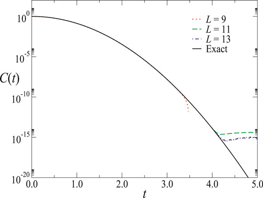
FIGURE 1. Time correlation function of a tagged spin in the TI model when $B=J=1.0$ for some chain sizes L, as indicated. Here and in the next figures $J=1$ is the energy unit. The exact solution is a Gaussian, which lies underneath the $L=13$ curve. [Figure from Guimarães et al. [17]].

FIGURE 2

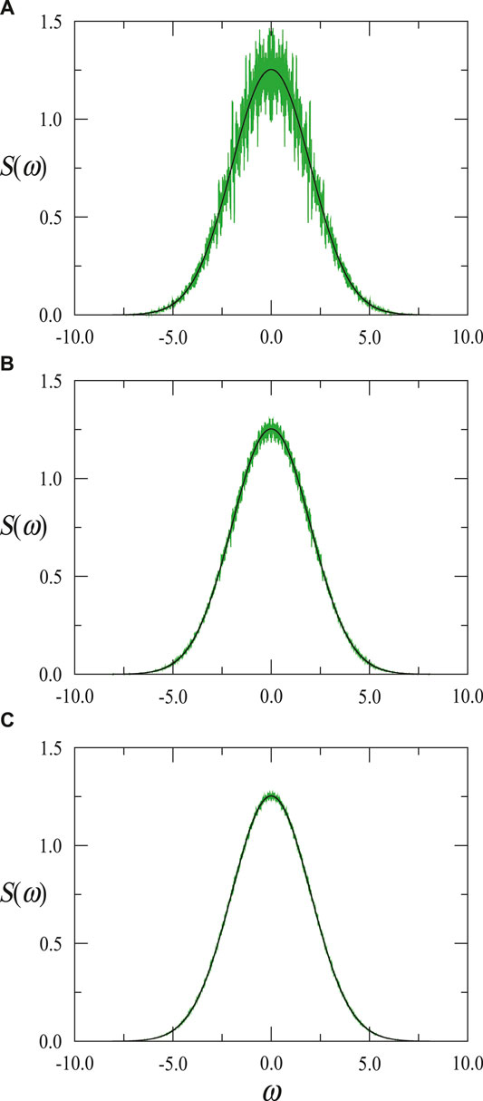
FIGURE 2. Spectral density for the TI model ($B=1$ and $J_2=0$) and different chain sizes. The plots are the time Fourier transforms of the curves in Figure 1. The curves for finite chains oscillate around the exact Gaussian result of the infinite chain. [From Ref. [17]]

In the following, consider the representative cases $B=0.5$, 1.0, and 2.0. These cases should cover the relevant possibilities for B in the transverse ANNNI model. Consider first $B=0.5$. The time correlation function $C\left(t\right)$ is shown in Figure 3 for different next-to-nearest neighbor couplings $J_2$. There are pairs of curves for a given $J_2$, dashed lines for $L=12$ and solid lines for $L=13$. Those two lines agree very well with each other for the range of time t displayed. The quantitative agreement between the $L=12$ and $L=13$ curves is an indication that within the accuracy used, the thermodynamic value has already been obtained. The features shown in Figure 3 are real and will not change in the thermodynamic limit. They possibly could be traced back to the rich ground-state phase diagram, however, a careful investigation is still necessary to clarify that point.

FIGURE 3

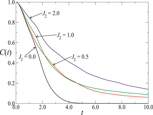
FIGURE 3. Time-dependent correlation function for $B=0.5$ and several values of the NNN coupling $J_2$ [17].

In general, the decay of $C\left(t\right)$ with time is slower for larger $J_2$. The corresponding spectral density is displayed in Figure 4, calculated for $L=13$. Other than the height near the origin $\omega =0$, the remaining plots should not change essentially for larger chain sizes, or at the thermodynamic limit. The distinctive feature is the enhancement of the central mode as $J_2$ increases.

FIGURE 4

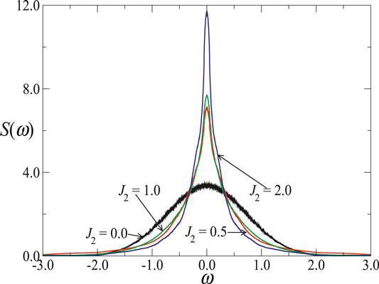
FIGURE 4. Spectral density for $B=0.5$ and several values of $J_2$. All the curves were obtained for chains with $L=12$ spins [17].

The time correlation function for $B=1$ is depicted in Figure 5 for several $J_2$. The curves shown are from $L=12$ and $L=13$. Note that for $J_2=0$ the calculation reproduces the known Gaussian solution of the TI model. When $J_2=0.5$, oscillations are present in $C\left(t\right)$. For $J_2\ge 1$ the curves decay at much slower rate. A careful examination of the figures shows oscillations of relatively small amplitudes. The spectral density $S\left(\omega \right)$ is shown in Figure 6, where the calculations were done with $L=13$. For $J_2=0$ the Gaussian of the TI model is reproduced. We observe an enhancement of the central model behavior as the values of $J_2$ are increased.

FIGURE 5

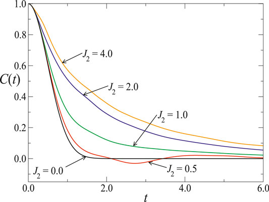
FIGURE 5. Time-dependent correlation function for $B=1$ and several values of $J_2$. The curves were obtained with $L=12$ and 13. See Ref. 17.

FIGURE 6

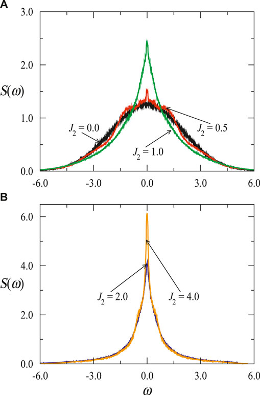
FIGURE 6. Spectral density for $B=1$ and several values of $J_2$, obtained for chains of length $L=13$. [From Ref. 17.]

Finally, consider the case where the transverse field is larger ($B=2$) than the Ising coupling. The time correlation function is shown in Figure 7 for several values of $J_2$. The curves were obtained from a chain of size $L=13$. For small values of $J_2$ the correlation function, $C\left(t\right)$, shows oscillations typical of collective mode, such as that found in the TI model ($J_2=0$). As $J_2$ becomes larger, the amplitude of the oscillations decreases. For large enough $J_2$, the system displays an enhancement of the central model.

FIGURE 7

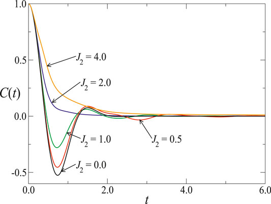
FIGURE 7. Time-dependent correlation function for $B=2.0$ and various values of $J_2$. The chain size is $L=13$. [From Ref. [17.]

Figure 8 depicts the corresponding spectral density $S\left(\omega \right)$ for the values of $J_2$ used in the previous figure. For $J_2=0$, the dynamics is dominated by the two-peak structure characteristic of collective mode. As $J_2$ increases, a reduction of the intensity of the peaks of the collective mode is observed in tandem with a growth of the central peak. For $J_2\ge 2$ the dynamics seems to be dominated entirely by the central mode.

FIGURE 8

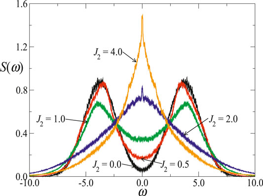
FIGURE 8. Spectral density for the case $B=2$ and several values of $J_2$. The plots were obtained for $L=12$ [17].

The recurrants ${\text{Δ}}_{\nu }$ of the method of recurrence relations are calculated numerically for $J_2=1$ and several values of B. First the moments μ are obtained by using Eq. 54. Next, use the conversion formulas Eq. 31. Table 1 shows some numerical results for the recurrants when $B=1.0$, and $J_2=1.0$, obtained for $L=11$, 12, and 13. The rightmost column shows the extrapolated value of ${\text{Δ}}_{\nu }$ for $L=\infty$. As can be seen, with relatively small chain sizes ($L\le 13$), one can infer the thermodynamic value of the lower-order recurrants. Higher order recurrants are still obtained, but with lesser accuracy.

TABLE 1

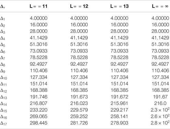
TABLE 1. Recurrants for the transverse ANNNI model, with $B=1.0$, $J_2=1.0$ and several chain sizes. The rightmost column is the extrapolation for the thermodynamic limit ($L=\infty$).

The results for the thermodynamic estimates of the recurrants are shown in Figure 9 for $B=1.0$ and various values for $J_2$. For $J_2=0$ the linear behavior that leads to Gaussian behavior is recovered [51]. As $J_2$ increases, ${\text{Δ}}_{\nu }$ increases at higher rates on the average and becomes rather erratic, therefore, it is difficult to predict a trend based on their behavior. Still the results shown are already the thermodynamic values, and it is very difficult to devise extrapolation schemes for the $\text{Δ}$. Notwithstanding, such an endeavor will not uncover any new physics in regard to the dynamics of the transverse ANNNI model considered here.

FIGURE 9

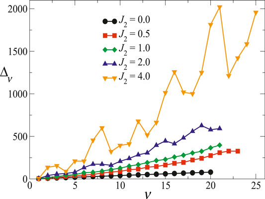
FIGURE 9. Recurrants of the infinite transverse ANNNI model with $B=1.0$ and several values of $J_2$ [17].

4 Summary and Perspectives

The dynamical correlation functions play a crucial role in the fluctuation-dissipation theorem and in the linear response theory. However, the calculation of those quantities is often a very complicated problem in itself. The method of recurrence relations is an exact procedure that allows one to obtain of time correlation functions, spectral densities, and dynamical structure factors. We have shown the main features of the method and the inherent difficulties one might encounter in an attempt to apply to a many-body problem. Another method that is showing great potential is exact diagonalization, a numerical method which relies mostly on computer capabilities. Nevertheless, the two methods can be used together, one complementing the other, to achieve progress in the calculation of dynamical correlation functions.

Author Contributions

The authors JF and OFAB declare that they planned and carried out the elaboration of this work with equal contribution from each author.

Conflict of Interest

The authors declare that the research was conducted in the absence of any commercial or financial relationships that could be construed as a potential conflict of interest.

Acknowledgments

This work was supported by FAPERJ and PROPPI-UFF (Brazilian agencies).

References

1. Callen HB, Welton TA. Irreversibility and generalized noise. Phys Rev E. (1951). 83:34–40. doi:10.1103/PhysRev.83.34

CrossRef Full Text | Google Scholar

2. Kubo R. The fluctuation-dissipation theorem. Rep Prog Phys. (1966). 29:255. doi:10.1088/0034-4885/29/1/306

CrossRef Full Text | Google Scholar

3. Lee MH. Orthogonalization processes by recurrence relations. Phys Rev Lett. (1982). 49:1072. doi:10.1103/PhysRevLett.49.1072

CrossRef Full Text | Google Scholar

4. Lee MH. Solutions of the generalized Langevin equation by a method of recurrence relations. Phys Rev B. (1982). 26:2547. doi:10.1103/PhysRevB.26.2547

PubMed Abstract | CrossRef Full Text | Google Scholar

5. Lee MH. Derivation of the generalized Langevin equation by a method of recurrence relations. J Math Phys. (1983). 24:2512. doi:10.1063/1.525628

CrossRef Full Text | Google Scholar

6. Grigolini P, Grosso G, Pastori Parravicini G, Sparpaglione M. Calculation of relaxation functions: a new development within the Mori formalism. Phys Rev B. (1983). 27:7342. doi:10.1103/PhysRevB.27.7342

PubMed Abstract | CrossRef Full Text | Google Scholar

7. Giordano M, Grigolini P, Leporini D, Marin P. Fast-computational approach to the evaluation of slow-motion EPR spectra in terms of a generalized Langevin equation. Phys Rev A. (1983). 28:2474. doi:10.1103/PhysRevA.28.2474

CrossRef Full Text | Google Scholar

8. Mori H. A continued-fraction representation of the time-correlation functions. Prog Theor Phys. (1965). 34:399–416. doi:10.1143/PTP.34.399

PubMed Abstract | CrossRef Full Text | Google Scholar

9. Zwanzig R. Statistical mechanics of irreversibility. In: Britten WE, Downs BW, Downs J, editors Lectures in theoretical physics.. New York, NY: Interscience (1961). p 106–141.

Google Scholar

10. Lee MH, Hong J, Florencio J. Method of recurrence relations and applications to many-body systems. Phys Scripta. (1987). T19:498. doi:10.1088/0031-8949/1987/T19B/029

CrossRef Full Text | Google Scholar

11. Viswanath VS, Müller G. The recursion method - application to many-body dynamics. In: Viswanath GS, Muller GM, editors Lectures notes in physics.. Berlin, Germany: Springer-Verlag (1994). 262 p.

Google Scholar

12. Balucani UU, Lee MH, Tognetti V. Dynamical correlations. Phys Rep. (2003). 373:409–492. doi:10.1016/S0370-1573(02)00430-1

CrossRef Full Text | Google Scholar

13. Sur A, Jasnow D, Lowe IJ. Spin dynamics for the one-dimensional XY model at infinite temperature. Phys Rev B. (1975). 12:3845. doi:10.1103/PhysRevB.12.3845

CrossRef Full Text | Google Scholar

14. Sur A, Lowe IJ. NMR line-shape calculation for a linear dipolar chain. Phys Rev B. (1975). 12:4597. doi:10.1103/PhysRevB.12.4597

PubMed Abstract | CrossRef Full Text | Google Scholar

15. Fabricius K, Löw U, Stolze J. Dynamic correlations of antiferromagnetic spin- XXZ chains at arbitrary temperature from complete diagonalization. Phys Rev B. (1997). 55:5833. doi:10.1103/PhysRevB.55.5833

CrossRef Full Text | Google Scholar

16. Boechat B, Cordeiro C, Florencio J, Sá Barreto FC, de Alcantara Bonfim OF. Dynamical behavior of the random-bond transverse Ising model with four-spin interactions. Phys Rev B. (2000). 61:14327. doi:10.1103/PhysRevB.61.14327

CrossRef Full Text | Google Scholar

17. Guimarães PRC, Plascak JA, de Alcantara Bonfim OF, Florencio J. Dynamics of the transverse Ising model with next-nearest-neighbor interactions. Phys Rev B. (2015). 92:042115. doi:10.1103/PhysRevE.92.042115

PubMed Abstract | CrossRef Full Text | Google Scholar

18. Perk JHH, Capel HW. Time-dependent correlation functions in the high-temperature limit for the XY-chain and the Ising-chainin a transverse magnetic field. J Appl Phys. (1979). 50:1771. doi:10.1063/1.327215

CrossRef Full Text | Google Scholar

19. Pires AST. The memory function formalism in the study of the dynamics of a many body system. Helv Phys Acta. (1988). 61:988–1006. doi:10.5169/seals-115978

Google Scholar

20. Plascak JA, Sá Barreto FC, Pires AST. Dynamics of the strong anisotropic three-dimensional Ising model in a transverse field. Phys Rev B. (1983). 27:523. doi:10.1103/PhysRevB.27.523

CrossRef Full Text | Google Scholar

21. Brandt U, Stolze J. High-temperature dynamics of the anisotropic Heisenberg chain studied by moment methods. Z Phyzik B. (1986). 64:327. doi:10.1007/BF01303603

CrossRef Full Text | Google Scholar

22. Böhm M, Leschke H. Dynamic spin-pair correlations in a Heisenberg chain at infinite temperature based on an extended short-time expansion. J Phys A. (1992). 25:1043. doi:10.1088/0305-4470/25/5/013

Google Scholar

23. Böhm M, Leschke H. Dynamical aspects of spin chains at infinite temperature for different spin quantum numbers. Physica A. (1993). 199:116–131. doi:10.1016/0378-4371(93)90101-9

CrossRef Full Text | Google Scholar

24. de Alcantara Bonfim OF, Reiter G. Breakdown of hydrodynamics in the classical 1D Heisenberg model. Phys Rev Lett. (1992). 69:367. doi:10.1103/PhysRevLett.69.367

PubMed Abstract | CrossRef Full Text | Google Scholar

25. Stolze J, Viswanath VS, Müller G. Dynamics of semi-infinite quantum spin chains at T = ∞. Z. Phyzik B (1992). 89:45–55. doi:10.1007/BF01320828

CrossRef Full Text | Google Scholar

26. Perk JHH, Au-Yang H. New results for the correlation functions of the Ising model and the transverse Ising chain. J Stat Phys. (2009). 135:599–619. doi:10.1007/s10955-009-9758-5

CrossRef Full Text | Google Scholar

27. Widera A, Gerbier F, F'́olling S, Gericke T, Mandel O, Bloch I. Coherent collisional spin dynamics in optical lattices. Phys Rev Lett. (2005). 95:190405. doi:10.1103/PhysRevLett.95.190405

PubMed Abstract | CrossRef Full Text | Google Scholar

28. Hild S, Fukuhara T, Schauss P, Zeiher J, Knap M, Demler E, et al. Far-from-equilibrium spin transport in Heisenberg quantum magnets. Phys Rev Lett. (2014). 113:147205. doi:10.1103/PhysRevLett.113.147205

PubMed Abstract | CrossRef Full Text | Google Scholar

29. Zhang H, Zhai1 Y, Chen X. Spin dynamics in one-dimensional optical lattices. J Phys B Atom Mol Opt Phys. (2014). 47:025301. doi:10.1088/0953-4075/47/2/025301

CrossRef Full Text | Google Scholar

30. Buyskikh S, Tagliacozzo L, Schuricht D, Hooley CA, Pekker D, Daley AJ. Spin models, dynamics, and criticality with atoms in tilted optical superlattices. Phys Rev Lett. (2019). 123:090401. doi:10.1103/PhysRevLett.123.090401

PubMed Abstract | CrossRef Full Text | Google Scholar

31. Kubo R. Statistical-mechanical theory of irreversible processes. I. General theory and simple applications to magnetic and conduction problems. J Phys Soc Japan. (1957). 12:570. doi:10.1143/JPSJ.12.570

CrossRef Full Text | Google Scholar

32. Lee MH. Derivation of the generalized Langevin equation by a method of recurrence relations. J. Math. Phys (1983). 24:2512. doi:10.1063/1.525628

CrossRef Full Text | Google Scholar

33. Lee MH, Hong J, Sharma NL. Time-dependent behavior of one-dimensional many-fermion models: comparison with two- and three-dimensional models. Phys Rev A. (1984). 29:1561. doi:10.1103/PhysRevA.29.1561

CrossRef Full Text | Google Scholar

34. Lee MH, Hong J. Recurrence relations and time evolution in the three-dimensional Sawada model. Phys Rev B. (1984). 30:6756. doi:10.1103/PhysRevB.30.6756

CrossRef Full Text | Google Scholar

35. Sharma NL. Response and relaxation of a dense electron gas in D dimensions at long wavelengths. Phys Rev B. (1992). 45:3552. doi:10.1103/PhysRevB.45.3552

PubMed Abstract | CrossRef Full Text | Google Scholar

36. Lee MH, Hong J. Time- and frequency-dependent behavior of a two-dimensional electron gas at long wavelengths. Phys Rev B. (1985). 32:7734. doi:10.1103/PhysRevB.32.7734

PubMed Abstract | CrossRef Full Text | Google Scholar

37. Florencio J, Lee MH. Exact time evolution of a classical harmonic-oscillator chain. Phys Rev A. (1985). 31:3231. doi:10.1103/PhysRevA.31.3231

PubMed Abstract | CrossRef Full Text | Google Scholar

38. Wierling A, Sawada I. Wave-number dependent current correlation for a harmonic oscillator. Phys Rev A. (2010). 82:051107. doi:10.1103/PhysRevE.82.051107

PubMed Abstract | CrossRef Full Text | Google Scholar

39. Wierling A. Dynamic structure factor of linear harmonic chain - a recurrence relation approach. Eur Phys J B. (2012). 85:20. doi:10.1140/epjb/e2011-20571-5

CrossRef Full Text | Google Scholar

40. Yu MB. Momentum autocorrelation function of an impurity in a classical oscillator chain with alternating masses – I General theory. Physica A. (2014). 398:252–63. doi:10.1016/j.physa.2013.11.023

CrossRef Full Text | Google Scholar

41. Yu MB. Momentum autocorrelation function of an impurity in a classical oscillator chain with alternating masses II. Illustrations. Physica A. (2015). 438:469–86. doi:10.1016/j.physa.2015.06.014

CrossRef Full Text | Google Scholar

42. Yu MB. Momentum autocorrelation function of a classic diatomic chain. Phys Lett. (2016). 380:3583–7. doi:10.1016/j.physleta.2016.08.042

CrossRef Full Text | Google Scholar

43. Yu MB. Momentum autocorrelation function of an impurity in a classical oscillator chain with alternating masses III. Some limiting cases. Physica A. (2016). 447:411–21. doi:10.1016/j.physa.2015.12.034

CrossRef Full Text | Google Scholar

44. Lee MH. Local dynamics in an infinite harmonic chain. Symmetry. (2016). 8:22. doi:10.3390/sym8040022

PubMed Abstract | CrossRef Full Text | Google Scholar

45. Yu MB. Analytical expressions for momentum autocorrelation function of a classic diatomic chain. Eur Phys J B. (2017). 90:87. doi:10.1140/epjb/e2017-70752-1

CrossRef Full Text | Google Scholar

46. Yu MB. Cut contribution to momentum autocorrelation function of an impurity in a classical diatomic chain. Eur Phys J B. (2018). 91:25. doi:10.1140/epjb/e2017-80402-3

CrossRef Full Text | Google Scholar

47. Mokshin AV. Relaxation processes in many particle systems – recurrence relations approach, discontinuity. Interdiscip J Discontinuity Nonlinearity Complexity. (2013). 2:43–56. doi:10.5890/DNC.2012.11.002

CrossRef Full Text | Google Scholar

48. Mokshin AV. Self-consistent approach to the description of relaxation processes in classical multiparticle systems. Theor Math Phys. (2015). 183:449–77. doi:10.1007/s11232-015-0274-2

CrossRef Full Text | Google Scholar

49. Sen S. Solving the Liouville equation for conservative systems: continued fraction formalism and a simple application. Physica A. (2006). 360:304–24. doi:10.1016/j.physa.2005.06.047

CrossRef Full Text | Google Scholar

50. Sawada I. Long-time tails of correlation and memory functions. Physica A. (2002). 315:14–25. doi:10.1016/S0378-4371(02)01231-1

CrossRef Full Text | Google Scholar

51. Florencio J, Lee MH. Relaxation functions, memory functions, and random forces in the one-dimensional spin-1/2 XY and transverse Ising models. Phys Rev B. (1987). 35:1835. doi:10.1103/PhysRevB.35.1835

PubMed Abstract | CrossRef Full Text | Google Scholar

52. Florencio J, Lee MH. Memory functions and relaxation functions of some spin systems. Nucl Phys B. (1988). 5A:250–54. doi:10.1016/0920-5632(88)90050-3

CrossRef Full Text | Google Scholar

53. Sawada I. Dynamics of the s=1/2 alternating chains at T = ∞. Phys Rev Lett. (1999). 83:1668. doi:10.1103/PhysRevLett.83.1668

CrossRef Full Text | Google Scholar

54. Florencio J, Lee MH, Hong JB. Time dependent transverse correlations in the Ising model in D dimensions. Braz J Phys. (2000). 30:725–30. doi:10.1590/S0103-97332000000400016

PubMed Abstract | CrossRef Full Text | Google Scholar

55. Nunes MES, Florencio J. Effects of disorder on the dynamics of the XY chain. Phys Rev B. (2003). 68:014406. doi:10.1103/PhysRevB.68.014406

CrossRef Full Text | Google Scholar

56. Nunes MES, Plascak JA, Florencio J. Spin dynamics of the quantum XY chain and ladder in a random field. Physica A. (2004). 332:1–14. doi:10.1016/j.physa.2003.10.049

CrossRef Full Text | Google Scholar

57. Plascak JA, Sá Barreto FC, Pires AST, Gonçalves LL. A continued-fraction representation for the one-dimensional transverse Ising model. J Phys C. (1983). 16:49. doi:10.1088/0022-33719/16/1/009

PubMed AbstractGoogle Scholar

58. Viswanath VS, Müller G. Recursion method in quantum spin dynamics: the art of terminating a continued fraction. J Appl Phys. (1990). 67:5486–8. doi:10.1063/1.345859

CrossRef Full Text | Google Scholar

59. Müller G, Thomas H, Beck H, Bonner JC. Quantum spin dynamics of the antiferromagnetic linear chain in zero and nonzero magnetic field. Phys Rev B. (1981). 24:1429. doi:10.1103/PhysRevB.24.1429

CrossRef Full Text | Google Scholar

60. Sawada I. High-energy excitations in aligned dimers. J Chem Phys Solids. (2001). 62:373–6. doi:10.1016/S0022-3697(00)00168-2

PubMed Abstract | CrossRef Full Text | Google Scholar

61. Sawada I. Dynamics of alternating spin chains and two-leg spin ladders with impurities. Physica B. (2003). 329-333:998–9. doi:10.1016/S0921-4526(02)02176-2

CrossRef Full Text | Google Scholar

62. Sen S, Cai ZX, Mahanti SD. Dynamical correlations and the direct summation method of evaluating infinite continued fractions. Phys Rev E. (1993). 47:273. doi:10.1103/PhysRevE.47.273

PubMed Abstract | CrossRef Full Text | Google Scholar

63. Liu ZQ, Kong XM, Chen XS. Effects of Gaussian disorder on the dynamics of the random transverse Ising model. Phys Rev B. (2006). 73:224412. doi:10.1103/PhysRevB.73.224412

CrossRef Full Text | Google Scholar

64. Yuan XJ, Kong XM, Xu ZB, Liu ZQ. Dynamics of the one-dimensional random transverse Ising model with next-nearest-neighbor interactions. Physica A. (2010). 389:242–8. doi:10.1016/j.physa.2009.08.021

PubMed Abstract | CrossRef Full Text | Google Scholar

65. Li YF, Kong XM. The dynamics of one-dimensional random quantum XY system with Dzyaloshinskii-Moriya interaction. Chin Phys B. (2013). 22:037502. doi:10.1088/1674-1056/22/3/037502

CrossRef Full Text | Google Scholar

66. Nunes MES, Silva EM, Martins PHL, Florencio J, Plascak JA. Dynamics of the one-dimensional isotropic Heisenberg model with Dzyaloshinskii-Moriya interaction in a random transverse field. Physica A. (2020). 541:123683. doi:10.1016/j.physa.2019.123683

CrossRef Full Text | Google Scholar

67. Silva EM. Dynamical class of a two-dimensional plasmonic Dirac system. Phys Rev E. (2015). 92:042146. doi:10.1103/PhysRevE.92.042146

PubMed Abstract | CrossRef Full Text | Google Scholar

68. Silva EM. Time evolution in a two-dimensional ultrarelativistic-like electron gas by recurrence relations method. Acta Phys Pol B. (2015). 46:1135. doi:10.5506/APhysPolB.46.1135

Google Scholar

69. Mokshin AV, Yulmetyev RM, Khusnutdinoff RM, Hänggi P. Analysis of the dynamics of liquid aluminium: recurrent relation approach. J Phys Condens Matter. (2007). 19:046209. doi:1088/0953-8984/19/4/046209

CrossRef Full Text | Google Scholar

70. Mokshin AV, Galimzyanov BN. Self-consistent description of local density dynamics in simple liquids. The case of molten lithium. J Phys Condens Matter. (2018). 30:085102. doi:10.1088/1361-648X/aaa7bc

PubMed Abstract | CrossRef Full Text | Google Scholar

71. Niemeijer T. Some exact calculations on a chain of spins 12. Physica. (1967). 36:377–419. doi:10.1016/0031-8914(67)90235-2

Google Scholar

72. Brandt U, Jacoby K. Exact results for the dynamics of one-dimensional spin-systems. Z Phyzik B. (1976). 25:181–7. doi:10.1007/BF01320179

CrossRef Full Text | Google Scholar

73. Brandt U, Jacoby K. The transverse correlation function of anisotropic XY-chains: exact results at T = ∞. Z Phys B. (1977). 26:245–52. doi:10.1007/BF01312930

CrossRef Full Text | Google Scholar

74. Capel HW, Perk JHH. Autocorrelation function of the x-component of the magnetization in the one-dimensional XY-model. Physica A. (1977). 87:211–42. doi:10.1016/0378-4371(77)90014-0

CrossRef Full Text | Google Scholar

75. Perk JHH, Capel HW. Transverse correlations in the inhomogenius XY-model at infinite temperature. Physica A. (1968). 92:1–49. doi:10.1016/0378-4371(84)90102-X

PubMed Abstract | CrossRef Full Text | Google Scholar

76. Lee MH, Florencio J, Hong J. Dynamic equivalence of a two-dimensional quantum electron gas and a classical harmonic oscillator chain with an impurity mass. J Phys A. (1989). 22:L331–L335. doi:10.1088/0305-4470/22/8/005

CrossRef Full Text | Google Scholar

77. Sen S, Long M, Florencio J, Cai ZX. A unique feature of some simple many body quantum spin systems. J Appl Phys. (1999). 73:5471. doi:10.1063/1.353669

CrossRef Full Text | Google Scholar

78. Florencio J, Sen S, Cai ZX. Quantum spin dynamics of the transverse Ising model in two dimensions. J Low Temp Phys. (1992). 89:561–4. doi:10.1007/BF00694087

PubMed Abstract | CrossRef Full Text | Google Scholar

79. Sen S, Long S, Florencio J, Cai ZX. A unique feature of some many-body quantum spin systems. J. Appl Phys. (1993). 73:3471. doi:10.1063/1.353669

CrossRef Full Text | Google Scholar

80. Sen S, Florencio J, Cai ZX. Long-time dynamics of the transverse Ising model – comparison with data on LiTbF₄. Mater Res Soc Symp Proc. (1993). 291:337. doi:10.1557/PROC-291-337

CrossRef Full Text | Google Scholar

81. Chen SX, Shen YY, Kong XM. Crossover of the dynamical behavior in two-dimensional random transverse Ising model. Phys Rev B. (2010). 82:174404. doi:10.1103/PhysRevB.82.174404

CrossRef Full Text | Google Scholar

82. Florencio J, Sen S, Cai ZX. Dynamic structure factor of the transverse Ising model in 2-D. J Phys Condens Matter. (1995). 7:1363. doi:10.1088/0953-8984/7/7/017

CrossRef Full Text | Google Scholar

83. Kotzler J, Neuhaus-Steinmetz H, Froese A, Gorlitz D. Relaxation-coupled order-parameter oscillation in a transverse Ising system. Phys Rev Lett. (1988). 60:647. doi:10.1103/PhysRevLett.60.647

PubMed Abstract | CrossRef Full Text | Google Scholar

84. Souza WL, Silva EM, Martins PHL. Dynamics of the spin-1/2 Ising two-leg ladder with four-spin plaquette interaction and transverse field. Phys Rev E. (2020). 101:042104. doi:10.1103/PhysRevE.101.042104

PubMed Abstract | CrossRef Full Text | Google Scholar

85. Khait I, Gazit S, Yao NY, Auerbach A. Spin transport of weakly disordered Heisenberg chain at infinite temperature. Phys Rev B. (2016). 93:224205. doi:10.1103/PhysRevB.93.224205

CrossRef Full Text | Google Scholar

86. Viswanath VS, Müller G. The recursion method applied to the T = 0 dynamics of the 1D s = 1/2 Heisenberg and XY models. J Appl Phys. (1991). 70:6178. doi:10.1063/1.350036

CrossRef Full Text | Google Scholar

87. Lee MH. Time evolution, relaxation function, and random force for a single-spin via the method of Mori. Can J Phys. (1983). 61:428–33. doi:10.1139/p83-054

CrossRef Full Text | Google Scholar

88. Sen S. Relaxation in nonlinear systems, nonconvergent infinite continued fractions and sensitive relaxation processes. Physica A. (2002). 315:150–5. doi:10.1016/S0378-4371(02)01365-1

CrossRef Full Text | Google Scholar

89. Sen S, Long M. Dynamical correlations in an s = 1/2 isotropic Heisenberg chain at T = ∞. Phys Rev B. (1992). 46:14617. doi:10.1103/PhysRevB.46.14617

PubMed Abstract | CrossRef Full Text | Google Scholar

90. Bohm M, Viswanath VS, Stolze J, Müller G. Spin diffusion in the one-dimensional s = 1/2 XXZ model at infinite temperature. Phys Rev B. (1994). 49:15669. doi:10.1103/PhysRevB.49.15669

PubMed Abstract | CrossRef Full Text | Google Scholar

91. Sen S. Relaxation in the s = 1/2 isotropic Heisenberg chain at T = ∞ towards a simple intuitive interpretation. Physica A. (1995). 222:195–204. doi:10.1016/0378-4371(95)00301-0

CrossRef Full Text | Google Scholar

92. Liu JM, Müller G. Infinite-temperature dynamics of the equivalent-neighbor XYZ model. Phys Rev E. (1990). 42:5854. doi:10.1103/PhysRevA.42.5854

PubMed Abstract | CrossRef Full Text | Google Scholar

93. Florencio J, de Alcantara Bonfim OF, Sá Barreto EFC. Dynamics of a transverse Ising model with four-spin interactions. Physica A. (1997). 235:523–33. doi:10.1016/S0378-4371(96)00299-3

PubMed Abstract | CrossRef Full Text | Google Scholar

94. Boechat B, Cordeiro C, de Alcantara Bonfim OF, Florencio J, Sá Barreto FC. Dynamical behavior of the four-body transverse Ising model with random bonds and fields. Braz J Phys. (2000). 30:693–6. doi:10.1590/S0103-97332000000400010

CrossRef Full Text | Google Scholar

95. de Alcantara Bonfim OF, Boechat B, Cordeiro C, Sá Barreto FC, Florencio J. Dynamics of the Ising chain with four-spin interactions in a disordered transverse magnetic field. J. Phys. Soc. Japan (2001). 70:829–33. doi:10.1143/JPSJ.70.829

Google Scholar

96. Florencio J, de Alcantara Bonfim OF. Temperature effects on the dynamics of the 1-D transverse Ising model with four-spin interactions. Physica A. (2004). 344:498–503. doi:10.1016/j.physa.2004.06.020

CrossRef Full Text | Google Scholar

97. Dzyaloshinskii I. A thermodynamic theory of weak ferromagnetism of antiferromagnetics. J Phys Chem Solid. (1958). 4:241–55. doi:10.1016/0022-3697(58)90076-3

CrossRef Full Text | Google Scholar

98. Moriya T. Anisotropic superexchange interaction and weak ferromagnetism. Phys Rev. (1960). 120:91. doi:10.1103/PhysRev.120.91

CrossRef Full Text | Google Scholar

99. Xia Q, Riseborough PS. One-dimensional Dzyaloshinski-Moriya antiferromagnets in an applied field. J Appl Phys. (1988). 63:4141. doi:10.1063/1.340521

CrossRef Full Text | Google Scholar

100. Lima LS, Pires AST. Spin dynamics in the one-dimensional antiferromagnetic with Dzyaloshinskii-Moriya interaction. J Magn Magn Mater. (2008). 320:2316–18. doi:10.1016/j.jmmm.2008.04.162

CrossRef Full Text | Google Scholar

101. Pires AST, Gouvêa ME. Dynamics of the one-dimensional quantum antiferromagnet with Dzyaloshinski-Moriya interactions. J Magn Magn Mater. (2000). 212:251–8. doi:10.1016/S0304-8853(99)00758-1

Google Scholar

102. Derzhko O, Verkholyak T. Dynamics of the spin-1/2 XY chain with Dzyaloshinskii-Moriya interaction. Physica B. (2005). 359:1403–5. doi:10.1016/j.physb.2005.01.438

CrossRef Full Text | Google Scholar

103. Derzhko O, Verkholyak T, Krokhmalskii T, Büttner H. Dynamic probes of quantum spin chains with the Dzyaloshinskii-Moriya interaction. Phys Rev B. (2006). 73:214407. doi:10.1103/PhysRevB.73.214407

CrossRef Full Text | Google Scholar

104. Verkholyak T, Derzhko O, Krokhmalskii T, Stolze J. Dynamic properties of quantum spin chains: simple route to complex behavior. Phys Rev B. (2007). 76:144418. doi:10.1103/PhysRevB.76.144418

CrossRef Full Text | Google Scholar

105. Nunes MES, Silva EM, Martins PHL, Plascak JA, Florencio J. Effects of a magnetic field on the dynamics of the one-dimensional Heisenberg model with Dzyaloshinskii-Moriya interactions. Phys Rev E. (2018). 98:042124. doi:10.1103/PhysRevE.98.042124

CrossRef Full Text | Google Scholar

106. Florencio J, Sá Barreto FC. Dynamics of the random one-dimensional transverse Ising model. Phys Rev B. (1999). 60:9555. doi:10.1103/PhysRevB.60.9555

CrossRef Full Text | Google Scholar

107. Pfeuty P. The one-dimensional Ising model with a transverse field. Ann Phys. (1970). 57:79–90. doi:10.1016/0003-4916(70)90270-8

CrossRef Full Text | Google Scholar