 Yousef I. Salamin
 Sergio Carbajo
94% of researchers rate our articles as excellent or good
Learn more about the work of our research integrity team to safeguard the quality of each article we publish.
Find out more
ORIGINAL RESEARCH article
Front. Phys. , 12 February 2019
Sec. Optics and Photonics
Volume 7 - 2019 | https://doi.org/10.3389/fphy.2019.00002
This article is part of the Research Topic Lasers in Accelerator Science and Secondary Emission Light Source Technology View all 7 articles
A simple model is introduced for the fields of a chirped laser pulse. As an application, dynamics of laser-acceleration of a single electron by the fields of a pulse, with a sin4 envelope, is investigated. Multi-GeV energy gains from interaction with pulses of peak intensity I0~1020 W/cm2, are reported.
Chirped pulse amplification (CPA) has revolutionized laser technology, elevating the output powers to the petawatt regime in the past thirty years or so [1, 2] and possibly beyond that soon [3]. Chirped optical pulses have many applications, especially in fiber-optic communication [4]. More recent applications include cooling of a mirror in cavity optomechanics [5]. Chirped pulses in acoustic and radar signal processing [6, 7] have a much longer history.
Chirped laser pulses have been employed in theoretical laser-acceleration investigations for some time now [8–11], but only a few experiments have shown some evidence of vacuum laser acceleration using few-cycle laser pulses [12, 13], let alone chirped few-cycle pulses. In any case, results based on the one-dimensional model, to be introduced in this paper, may be compared to those stemming from the full three-dimensional calculations, only qualitatively.
Popular models of chirping the frequency, ω, of a wave include letting ω = ω0 + bt (a linear chirp) in which the parameter b has the unit of s−2, t is the time, and ω0 is the initial frequency (at t=0) [14–17]. Likewise, a quadratic chirp is obtained by taking , in which b has a unit of s−3, or , with b1 and b2 having the units s−2 and s−3, respectively, and so on.
In some recent applications, chirping the frequency of a laser pulse, of frequency ω0 and wavenumber k0 and propagating along the z-direction, has been modeled by replacing η = ω0t − k0z with η + bη2 (linear, with b a dimensionless parameter) and quadratic (η → η + bη3). This work adopts the approach based on the variable η [18–21].
So, to model the relevant experimental situation and account for the chirp, time dependence in the frequency has been altered by hand, directly by adding terms which contain the time t and chirp parameters, or indirectly through changing η. This seems to work quite well, for a linear chirp, to model what transpires when a laser pulse is, for example, passed through a linear medium of the right properties, including the right index of refraction. The model we put forward in this work accounts for all orders of chirp in a unified way and employing a single parameter, thus lowering the degree of arbitrariness in describing the chirp. It allows for the use of non-linear media to produce chirps of orders above the linear, which stands a good chance of opening the door for more novel applications in the field. Precise control over the temporal chirp of ultrashort pulses is possible today employing devices such as acousto-optic programmable dispersive filters, which are capable of tailoring the spectral phase- and amplitude-phase to several orders [22].
Some background material, of direct relevance to this work, is briefly reviewed in section 2, before the fields of a chirped laser pulse are introduced in section 3. Dynamics of a single electron subjected to the chirped pulse will be discussed in section 4. Finally, a summary and our main conclusions will be given in section FF 5.
In a typical textbook exercise on electromagnetic waves, one is asked to show that any well-behaved function f(η) satisfies the full set of Maxwell's equations in a vacuum, exactly [23]. Based on this, the following qualify for adequately representing the linearly-polarized transverse fields of an un-chirped pulse (in SI units) [24]
where φ0 is an initial phase, E0 is a constant amplitude, c is the speed of light in vacuum, and and ŷ are unit vectors in the (transverse) x− and y−directions, respectively. For a few-cycle pulse, φ0 serves as the carrier envelope phase (CEP). The fields in Equations (1, 2) are non-zero only for η ∈ [0, 2Nπ], in which N (giving the number of η−cycles in the pulse) is an integer chosen to ensure that the fields vanish at η = 0 and η = 2Nπ. The intensity of such a pulse will be calculated as the time-average of the Poynting vector in the focal plane. With μ0 and ε0 standing, respectively, for the permeability and permittivity of free space, the pulse intensity may be calculated from
For our purposes in this work, the number of field cycles (in η) will be N ≥ 3, for which the electric field amplitude will be given by
Our aim in this paper is to introduce a simple model for chirping the frequency of the fields given by Equations (1, 2) and to employ the chirped fields in investigating the dynamics of a single electron subjected to the pulse they represent. The chirped fields will be discussed briefly in the next section.
The starting point is the observation that, when one lets
in the argument of the sin oscillation in Equations (1, 2) one gets what resembles a linear chirp, a quadratic chirp, and so on, if the series is truncated at the second term, at the third term, …etc., respectively. The expansion in (5) is valid so long as |bη| < 1. So, provided this convergence condition is adhered to faithfully, the fields
can be employed as chirped counterparts for (1) and (2). These fields also satisfy the full set of Maxwell's equations, exactly. Note that the model depends upon a single dimensionless parameter, b. A chirp, modeled in this fashion, destroys the symmetry of the un-chirped oscillation merely slightly, but sensitively enough to circumvent the Lawson-Woodward theorem [25–28] and result in net electron acceleration, as will be shown in the next section.
Equations (6, 7) have not been produced rigorously. Rather, they have been constructed with the aim of encompassing linear chirp along with higher-order chirps in a single equation. In principle, they also lead to electron dynamics that can be handled analytically, and to results that may be interpreted easily. The choice expressed by Equation (5) is not unique. The above-mentioned goals can be achieved by other alternative, but not totally unrelated, models such as exponential, logarithmic, and power chirps [29].
Next the dynamics of a single electron (mass m and charge −e) injected along +z, the propagation direction of the pulse, is investigated. Without any loss of generality, the assumption is made here that the front of the pulse will catch up with the electron exactly at t = 0, and precisely at the instant it is at the origin of coordinates. This assumption may be difficult to realize experimentally, in which case the delay between the particle and the front of the pulse must be taken into account. This merely results in a set of initial conditions different from the ones employed below, if the above assumption is made. In this model, we assume no laser-electron timing jitter. That is, we select an electron injection phase for the chirped electric field to evidence the potential theoretical energy gain a single electron may experience. In practical terms, if we consider optical wavelengths (e.g., λ ~ 1 μm) to achieve the high intensity regime presented here, we would require the injection phase error to be ~ λ/10 or smaller, or equivalently, lower than ~ 300 attoseconds for a single electron. These timing error levels are currently achievable using any general self-injected scheme because the electron originates from a process triggered by the same accelerating laser fields.
Assuming no delay, the electron will have the relativistic injection kinetic energy , where and β0 is the injection (initial) speed scaled by c. The relativistic Newton-Lorentz equations of motion (or energy-momentum transfer equations) of the electron may be combined to give
where γ = (1 − β2)−1/2 is the Lorentz factor of the electron and β is its velocity vector scaled by c. Equation (8) possess analytic, but admittedly cumbersome, solutions for linear and quadratic chirps, in terms of Fresnel cosine and sine integral functions [20, 21]. Beyond that, resorting to numerical methods seems inevitable, which will be done in this work. The vector Equation (8) is equivalent to three component (coupled) differential equations. Our numerical calculations employ a Runge-Kutta-based Mathematica code developed by one of us and used over the years [18–21] to solve problems involving laser-matter interactions. Note that, in principle, a single integration of Equation (8) yields the Lorentz factor γ of the electron (or its energy scaled by the rest energy mc2) which then may be used to find the kinetic energy K = (γ − 1)mc2. A second integration, employing the appropriate initial conditions, then yields the particle trajectory.
Some examples are taken up next. Specifically, dynamics of a single electron injected with initial kinetic energy K0 ~ 2 MeV (γ0 = 5) and subsequently submitted to a laser pulse of N cycles in η, and whose intensity is I0, will be discussed. The tacit assumption is made here that the electrons are produced, by whatever means, outside the region of interaction with the laser and subsequently guided to where they interact as described.
Behavior of the exit kinetic energy of the electron, following interaction with the laser pulse, as a function of the chirp parameter, is shown in Figure 1. The rows are for N = 3, 4, and 5, respectively, and the columns are for and 1021 W/cm2, respectively. Note first that the range of b values decreases with increasing N, reflecting the role played by the convergence condition |bη| < 1. Second, the exit kinetic energy Kexit → K0 in the limit of b → 0, implying zero gain by the electron, as predicted by the Lawson-Woodward theorem [25–27]. Due to the fact that K ∝ I0, the values of Kexit in (d)-(f) are 10 times the corresponding values in (a)-(c). Finally, note that the exit kinetic energy values are sensitive to variations in b.
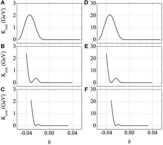
Figure 1. (Color online) (A–C) Exit kinetic energy of a single electron injected axially for interaction with a 1020 W/cm2 chirped pulse containing 3, 4, and 5 η-cycles, respectively, vs. the chirp parameter b. The electron is assumed to have been injected axially with kinetic energy K0 ~ 2 MeV (γ0 = 5) and φ0 = 0. (D–F) Same as (A–C), respectively, but for pulse peak intensity W/cm2.
In Figure 2, the un-chirped and chirped normalized electric fields are shown together for a pulse of 5 cycles in η. It is clear that the symmetry of the pulse is partially destroyed by chirping. Corresponding positive and negative parts, of each oscillation in η, are no longer identical. Thus, for example, the acceleration which results from interaction of an electron with a negative part of an oscillation, does not get canceled by the deceleration resulting from interaction with the corresponding, but no longer identical, positive part. The end result is, therefore, one of net acceleration or, equivalently, net energy gain by the electron from the pulse.
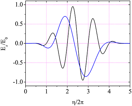
Figure 2. (Color online) Scaled electric field, Ex/E0, vs. the number of η−cycles for the un-chirped (black, b = 0) and chirped (blue, b = −0.038) pulses. The graphs have been produced using λ = 1 μm and φ0 = 0.
The example of single-electron acceleration by a 5-cycle chirped pulse, with a chirp parameter b = −0.038, is analyzed further by studying Figures 3, 4. Evolution of the kinetic energy of the electron, with η, is shown in Figure 3. The interaction results in a gain of 2.482 GeV by the electron. The comments presented in the previous paragraph are further supported by Figure 3B, which displays the normalized electric field seen by the electron during interaction with the pulse, including the correlation between the lack of symmetry of the field and the net energy gain by the electron. Note that, viewed as a function of η, the time t = η/ω0 + z(η)/c. This is obviously a transcendental equation that can best be shown graphically. The t vs. η relationship is shown in Figure 3C. From this figure, the total laboratory time of laser-particle interaction is less than 0.446 ns, for the parameters used. This interaction time is equivalent to about 133796 T, where T = λ/c is the laser period.
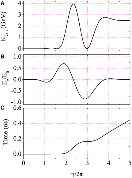
Figure 3. (Color online) (A) Evolution of the electron kinetic energy with η during interaction with a 1020 W/cm2 chirped pulse (b = −0.038) of wavelength λ = 1 μm, φ0 = 0, and containing 5 cycles in η. (B) The normalized electric field seen by the electron during interaction with the pulse. (C) The transcendental relation connecting the laboratory time t with η. The electron is injected axially with kinetic energy K0 ~ 2 MeV (γ0 = 5). Front of the pulse is assumed to have caught up with the electron at t = 0, at the origin of coordinates.
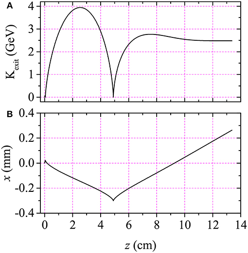
Figure 4. (Color online) (A) Same as Figure 3A, except here the kinetic energy evolution is plotted against the axial excursion distance, z. (B) Trajectory of the same electron in the xz−plane (the polarization plane).
Moving on to Figure 4, more interesting information may be extracted regarding the example just considered. Figure 4A is similar to Figure 3A, except here the kinetic energy evolution is shown as a function of the excursion distance along the direction of propagation of the pulse. First, note the obvious correlation between the two curves displayed in Figures 3A, 4A. Second, during the electron interaction with the pulse, its trajectory extends an axial distance Δz ~ 13.38 cm. Its exit kinetic energy, in this particular example, is equivalent to an energy gain of roughly ΔK ≡ Kexit − K0 ~ 2.480 GeV. These numbers predict an energy gradient of ΔK/Δz ~ 18.533 GeV/m, or more than 185 times the natural limit (~ 100 MeV/m) on the performance of the corresponding conventional (linear) electron accelerator.
Figure 4B shows the actual trajectory of the electron in the example subject of the discussion above. It is a typical 2D trajectory one would expect for an electron interacting with a linearly-polarized laser pulse. Effect of the x−polarized electric field is obvious in accelerating the electron transversely, relative to the pulse propagation direction. At the same time the forward excursion made by the electron is quite substantial. Once the electron is left behind the pulse, it follows a straight line trajectory whose direction is the same as the direction of its final (exit) momentum vector. For the example at hand, the scattering angle is about , with the direction of propagation of the pulse.
We acknowledge that, for the results presented above, the interaction lengths and times between a (semi)relativistic electron and a laser are very long compared to what can currently be achieved with Fourier optics in free-space, in order to achieve such relativistic intensity levels. One possible avenue of investigation to overcome this challenge is the use of spatially and spectrally shaped beams, tailored to abruptly focus and defocus from high on-axis intensity [30]. A single electron at rest would naturally exhibit much shorter interaction lengths that are more realistic under conventional Fourier optics. In Figure 5 results similar to those of Figure 4 are displayed, but for an electron accelerated from rest (β0 = 0, γ0 = 1). According to Figure 5A the electron gets accelerated from rest to a kinetic energy ~ 251 MeV, over an axial excursion distance of Δz ~ 1.36 mm, and 4.56 ps interaction time. These numbers yield an acceleration gradient of 183.8 GeV/m, ten times that of the case displayed in Figure 4. From Figure 5B one also reads that the maximum transverse excursion of the electron is about 26.7 μm. Finally, the scattering angle of the electron accelerated from rest is roughly 3.7°.
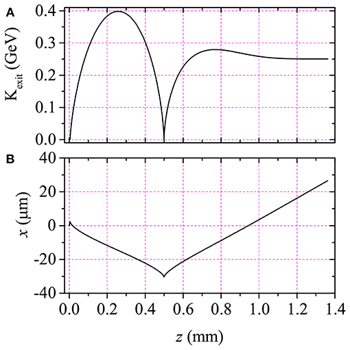
Figure 5. (Color online) Same as Figure 4, albeit for acceleration from rest (γ0 = 1).
Attention in this work has been focused on a somewhat generalized model for chirping the frequency of a plane-wave laser pulse of finite axial extension. The un-chirped linearly-polarized electric field of the pulse is a simple sin oscillation under a sin4 pulse envelope. This representation is quite idealized. A more realistic model ought to take into account the finite extension of the pulse in both space and time. Despite the observation that the pulse has a finite spatial extension in the axial (propagation) direction, it is still plane-wave in character in the transverse plane. This only strengthens the case for the need to adopt a more realistic model for description of the fields of the laser pulse [31–33].
The model also ignores existence of the axial field components and the Gouy phase [34]. These are important pulse attributes that must be included in any proper description of the fields of a high-power, tightly-focused and ultra-short laser pulse [31–33].
Finally, the examples employed to demonstrate utility of our model for the chirped fields have been limited to free-space electron acceleration, employing laser field intensities of about 1021 W/cm2. For these reasons, radiation-reaction effects have been ignored. Proper account of the radiation-reaction effects requires resort to quantum electrodynamical methods, which fall beyond the scope of the present work. Recent calculations have demonstrated that such effects can be significant in plasma-based laser acceleration of electrons, when the laser intensity employed exceeds 1023 W/cm2 [35].
YS is the conceptual author of the presented work. YS developed the methods. YS and SC contributed to the theoretical results and to the composition of the manuscript.
The authors declare that the research was conducted in the absence of any commercial or financial relationships that could be construed as a potential conflict of interest.
This work was supported by the Department of Energy, Laboratory Directed Research and Development program at SLAC National Accelerator Laboratory, under contract DE-AC02-76SF00515.
1. Strickland D, Mourou G. Compression of amplified chirped optical pulses. Opt Commun. (1985) 55:447–9. doi: 10.1016/0030-4018(85)90151-8
2. Yanovsky V, Chvykov V, Kalinchenko G, Rousseau P, Planchon T, Matsuoka T, et al. Ultra-high intensity- 300-TW laser at 0.1 Hz repetition rate. Opt Express (2008) 16:2109–14. doi: 10.1364/OE.16.002109
3. Gales S, Tanaka KA, Balabanski DL, Negoita F, Stutman D, Tesileanu O, et al. The extreme light infrastructurenuclear physics (ELI-NP) facility: new horizons in physics with 10 PW ultra-intense lasers and 20 MeV brilliant gamma beams. Rep Prog Phys. (2018) 81:094301. doi: 10.1088/1361-6633/aacfe8
4. Kim Y, Kim DY. Dual chirped optical pulses from a phase-modulated laser. Opt Express (2007) 15:16357–66. doi: 10.1364/OE.15.016357
5. Liao JQ, Law CK. Cooling of a mirror in cavity optomechanics with a chirped pulse. Phys Rev A (2011) 84:053838. doi: 10.1103/PhysRevA.84.053838
8. Singh KP. Electron acceleration by a chirped short intense laser pulse in vacuum. Appl Phys Lett. (2005) 87:254102. doi: 10.1063/1.2149984
9. Li JX, Zang WP, Tian JG. Electron acceleration in vacuum induced by a tightly focused chirped laser pulse. Appl Phys Lett. (2010) 96:031103. doi: 10.1063/1.3294634
10. Jin L, Wen M, Shen B. Nanocontrol of single dense energetic electron sheet in a chirped pulse with critical relativistic intensity. Phys Rev Spec Top Accel Beams (2013) 16:051301. doi: 10.1103/PhysRevSTAB.16.051301
11. Rezaei-Pandari M, Akhyani M, Jahangiri F, Niknam AR, Massudi R. Effect of temporal asymmetry of the laser pulse on electron acceleration in vacuum. Opt Commun. (2018) 429:46–52. doi: 10.1016/j.optcom.2018.07.081
12. Carbajo S, Nanni EA, Wong LJ, Moriena G, Keathley PD, Laurent G, et al. Direct longitudinal laser acceleration of electrons in free space. Phys Rev Accel Beams (2016) 19:021303. doi: 10.1103/PhysRevAccelBeams.19.021303
13. Chalopin B, Arbouet A. Ultrafast laser optical pinball. Nat Phys. (2018) 14:110–1. doi: 10.1038/nphys4314
14. Sohbatzadeh F, Mirzanejhad S, Ghasemi M. Electron acceleration by a chirped Gaussian laser pulse in vacuum. Phys Plasmas (2006) 13:123108. doi: 10.1063/1.2405345
15. Sohbatzadeh F, Mirzanejhad S, Aku H. Synchronization scheme in electron vacuum acceleration by a chirped Gaussian laser pulse. Phys Plasmas (2009) 16:023106. doi: 10.1063/1.3077666
16. Sohbatzadeh F, Mirzanejhad S, Aku H, Ashouri S. Chirped Gaussian laser beam parameters in paraxial approximation. Phys Plasmas (2010) 17:083108. doi: 10.1063/1.3464478
17. Sohbatzadeh F, Aku H. Polarization effect of a chirped Gaussian laser pulse on the electron bunch acceleration. J Plasma Phys. (2011) 77:3950. doi: 10.1017/S0022377809990407
18. Galow BJ, Salamin YI, Liseykina TV, Harman Z, Keitel CH. Dense monoenergetic proton beams from chirped laser-plasma interaction. Phys Rev Lett. (2011) 107:185002. doi: 10.1103/PhysRevLett.107.185002
19. Salamin YI. Net electron energy gain from interaction with a chirped “plane-wave” laser pulse. Phys Lett A (2012) 376:2442–5. doi: 10.1016/j.physleta.2012.06.020
20. Salamin YI, Jisrawi NM. Electron laser acceleration in vacuum by a quadratically chirped laser pulse. J Phys B Atom Mol Opt Phys. (2014) 47:025601. doi: 10.1088/0953-4075/47/2/025601
21. Jisrawi NM, Galow BJ, Salamin YI. Simulation of the relativistic electron dynamics and acceleration in a linearly-chirped laser pulse. Laser Part Beams (2014) 32:671–80. doi: 10.1017/S0263034614000603
22. Tournois P. Acousto-optic programmable dispersive filter for adaptive compensation of group delay time dispersion in laser systems. Opt Commun. (1997) 140:245–9.
24. Angioi A, Mackenroth F, DiPiazza A. Nonlinear single Compton scattering of an electron wave packet. Phys Rev A (2016) 93:052102. doi: 10.1103/PhysRevA.93.052102
25. Woodward PM. A method of calculating the field over a plane aperture required to produce a given polar diagram. J Inst Electric Eng. (1947) 93:1554–8.
27. Esarey E, Sprangle P, Krall J. Laser acceleration of electrons in vacuum. Phys Rev E (1995) 52:5443–53. doi: 10.1103/PhysRevE.52.5443
28. Hartemann FV, Fochs SN, LeSage GP, Luhmann NC, Woodworth JG, Perry MD, et al. Nonlinear ponderomotive scattering of relativistic electrons by an intense laser field at focus. Phys Rev E (1995) 51:4833–43. doi: 10.1103/PhysRevE.51.4833
29. Darowicki K, Ślepski P. Determination of electrode impedance by means of exponential chirp signal. Electrochem Commun. (2004) 6:898–902. doi: 10.1016/j.elecom.2004.06.013
30. Wong LJ, Kaminer I. Abruptly focusing and defocusing needles of light and closed-Form electromagnetic wavepackets. ACS Photon. (2017) 4:1131–7. doi: 10.1021/acsphotonics.6b01037
31. Salamin YI. Simple analytical derivation of the fields of an ultrashort tightly focused linearly polarized laser pulse. Phys Rev A (2015) 92:063818. doi: 10.1103/PhysRevA.92.063818
32. Salamin YI. Fields and propagation characteristics in vacuum of an ultrashort tightly focused radially polarized laser pulse. Phys Rev A (2015) 92:053836. doi: 10.1103/PhysRevA.92.053836
33. Li JX, Salamin YI, Hatsagortsyan KZ, Keitel CH. Fields of an ultrashort tightly focused laser pulse. J Opt Soc Am B (2016) 33:405–11. doi: 10.1364/JOSAB.33.000405
34. Paschotta R. Beam quality deterioration of lasers caused by intracavity beam distortions. Opt Express (2006) 14:6069–74. doi: 10.1364/OE.14.006069
Keywords: chirped pulse, laser acceleration, few cycle pulse, relativistic electrons, tightly focused
PACS numbers: 42.65.-k, 42.50.Vk, 52.75.Di
Citation: Salamin YI and Carbajo S (2019) A Simple Model for the Fields of a Chirped Laser Pulse With Application to Electron Laser Acceleration. Front. Phys. 7:2. doi: 10.3389/fphy.2019.00002
Received: 31 July 2018; Accepted: 07 January 2019;
Published: 12 February 2019.
Edited by:
Narayana Rao Desai, University of Hyderabad, IndiaReviewed by:
Ilia L. Rasskazov, University of Rochester, United StatesCopyright © 2019 Salamin and Carbajo. This is an open-access article distributed under the terms of the Creative Commons Attribution License (CC BY). The use, distribution or reproduction in other forums is permitted, provided the original author(s) and the copyright owner(s) are credited and that the original publication in this journal is cited, in accordance with accepted academic practice. No use, distribution or reproduction is permitted which does not comply with these terms.
*Correspondence: Yousef I. Salamin, eXNhbGFtaW5AYXVzLmVkdQ==
Disclaimer: All claims expressed in this article are solely those of the authors and do not necessarily represent those of their affiliated organizations, or those of the publisher, the editors and the reviewers. Any product that may be evaluated in this article or claim that may be made by its manufacturer is not guaranteed or endorsed by the publisher.
Research integrity at Frontiers
Learn more about the work of our research integrity team to safeguard the quality of each article we publish.