Monitoring Betaine Using Interval Time Between Events Control Chart

A generalization of moving average (MA) control chart for the exponential distribution under classical statistics is presented in this article. The designing of the MA control chart for the exponential distribution under neutrosophic statistics is also presented. A Monte Carlo simulation under neutrosophic is introduced and applied to determine the neutrosophic control limits coefficients and neutrosophic average run length and neutrosophic standard deviation for various shifts. The application of the proposed chart is given using Betaine data. The comparison and real example studies show the efficiency of the proposed chart over the existing charts.

Introduction

Although the Shewhart control charts have been applied widely due to their operational simplicity, these control charts are nevertheless designed and implemented under the assumption that the quality of interest follows the symmetrical distribution. In addition, the Shewhart control charts detect only a big shift in the process. In practice, such as in the chemical process, accelerated life testing and in the healthcare department, the quality of interest does not follow the normal distribution. The Shewhart control charts cannot be applied when the data is skewed, see Derya and Canan (1). Nelson (2) proposed a control chart for the Weibull distribution. Bai and Choi (3) worked on a control chart for skewed data. Zhang et al. (4) proposed a chart for the gamma distribution. Rahali et al. (5) presented a chart for various distributions. More details for such control charts can be seen in Choobineh and Ballard (6). Santiago and Smith (7) used Nelson (8) transformation to convert exponential distribution data to normal and presented the chart to monitor the time between events. Aslam et al. (9) extended Santiago and Smith (7) chart for the repetitive sampling. More details about this type of control charts can be seen in Zhang et al. (4), Aksoy (10), and Borror et al. (11).

The control chart based on moving average (MA), exponentially weighted moving average (EWMA), and cumulative sum (CUSUM) statistics is more sensitive to detecting a small shift in the process. An economic model for the MA chart is introduced by Chen and Yang (12). Wong et al. (13) studied the sensitivity of the MA chart. Khoo and Wong (14) and Areepong (15) proposed an MA chart using a double sampling scheme. Mohsin et al. (16) presented the MA chart using loss function. Alghamdi et al. (17) designed the MA chart for the Weibull distribution.

The fuzzy approach is applied when uncertainty in observations or parameters in presented. According to Khademi and Amirzadeh (18), “fuzzy data exist ubiquitously in the modern manufacturing process.” The fuzzy-based control charts are applied to monitor the process when the data have uncertain observations. Intaramo and Pongpullponsak (19) presented a control chart using the alpha cut approach. Faraz and Moghadam (20) proposed the chart using the fuzzy approach. Zarandi et al. (21) proposed the hybrid chart using fuzzy logic. Faraz et al. (22) proposed the variable chart under an uncertainty setting. Wang and Hryniewicz (23) proposed a fuzzy control chart using the bootstrap approach. Kaya et al. (24) proposed a fuzzy chart for individual observation.

Neutrosophic statistics (NS), which is the extension of classical statistics, works on the idea of neutrosophic numbers. In practice, in our world, the more indeterminate data are obtained than the determinate data; therefore, the use of NS becomes important to deal with such data, see Smarandache (25). The NS can be applied when the data have the neutrosophic numbers. Chen et al. (26, 27) worked on NS and applied in rock engineering. Aslam et al. (28) proposed the Shewhart control charts using NS. Aslam (29) designed the charts for an exponential distribution using NS. More information on NS can be seen in Alhabib et al. (30) and Chutia et al. (31). More applications of the neutrosophic numbers can be seen in Ye (32, 33), Ye et al. (34), Mondal et al. (35, 36), Pramanik and Banerjee (37), and Maiti et al. (38).

By exploring the literature and to the best of our knowledge, there is no work on MA control chart using the exponential distribution under NS. In this article, we use Nelson (8) transformation to propose a chart for the exponential distribution. The neutrosophic Monte Carlo (NMC) will be introduced for the MA chart. We expect that the proposed neutrosophic MA (NMA) chart for neutrosophic exponential distribution (NED) will perform better than the MA chart for neutrosophic distribution under classical statistics. This article is structured as follows: designs of the proposed charts are given in section “Design of the Proposed Charts,” the comparative study is given in section “Comparative Study,” the application of the proposed charts is given in section “Application of Proposed Chart Using Betaine Data,” and some concluding remarks are given in the last section.

Design of the Proposed Charts

Let the neutrosophic time between event T_N = T + A_NI_N; I_N ∈ [I_L,I_U], where T shows the time between event under classical statistics, A_NI_N denotes the indeterminate part, and I_N ∈ [I_L,I_U] denotes the indeterminacy interval follows NED having the neutrosophic scale parameter θ_N ∈ [θ_L,θ_U]. Aslam (29) introduced the neutrosophic probability density function (NPDF) following form of NED:

$\text{f}\left({\text{t}}_{\text{N}}\right)=\frac{1}{{\mathrm{\theta }}_{\text{N}}}{\text{e}}^{-{\text{t}}_{\text{N}}/{\mathrm{\theta }}_{\text{N}}};{\text{t}}_{\text{N}}\ge 0,T_N\in [T_L,T_U],{\mathrm{\theta }}_{\text{N}}\in [{\mathrm{\theta }}_L,{\mathrm{\theta }}_U](1)$

where Γ(t_N) denotes the gamma function, see Aslam and Arif (39) for details. The neutrosophic commutative distribution function (NCDF) is given by,

$\text{P}(T_N\le t_N)+1-\exp (-{\text{t}}_{\text{N}}/{\mathrm{\theta }}_{\text{N}});{\text{t}}_{\text{N}}\ge 0,T_N\in [T_L,T_U],{\mathrm{\theta }}_{\text{N}}\in [{\mathrm{\theta }}_L,{\mathrm{\theta }}_U](2)$

The neutrosophic forms of the NPDF and NCDF of NED are written as follows:

$f\left(t_N\right)=f\left(t\right)+B_N{I}_N;I_N\in [I_L,I_U](3)$

and

$F\left(t_N\right)=F\left(t\right)+C_N{I}_N;I_N\in [I_L,I_U](4)$

where f(t) and F(t) are PDF and CDF of the exponential distribution under classical statistics. The NPDF and NGD become classical exponential distribution if no indeterminacy is found in the data. According to Nelson (8) and Santiago and Smith (7), if T_N ∈ [T_L,T_U] follows the NED, then $T_N^{*}=T_N^{1/{\mathrm{\beta }}_N};T_N^{*}\in [T_L^{*},T_U^{*}]$ follows the neutrosophic Weibull distribution with neutrosophic shape parameter β_N ∈ [β_L,β_U] and neutrosophic scale parameter ${\mathrm{\theta }}_N^{1/{\mathrm{\beta }}_N}$. Note here that the neutrosophic Weibull distribution becomes approximately neutrosophic normal distribution when β_N ∈ [3.6,3.6] having the following neutrosophic mean and variance:

${\mathrm{\mu }}_N={\mathrm{\theta }}_{0N}^{*}\mathrm{\Gamma }\left(1+\frac{1}{3.6}\right);{\mathrm{\theta }}_{0N}^{*}\in [{\mathrm{\theta }}_{0L}^{*},{\mathrm{\theta }}_{0U}^{*}](5)$

${\mathrm{\sigma }}_N^2={\mathrm{\theta }}_{0N}^{*2}\left[\mathrm{\Gamma }\left(1+\frac{2}{3.6}\right)-\mathrm{\Gamma }{\left(1+\frac{1}{3.6}\right)}^2\right];{\mathrm{\theta }}_{0N}^{*}\in [{\mathrm{\theta }}_{0L}^{*},{\mathrm{\theta }}_{0U}^{*}](6)$

where ${\mathrm{\theta }}_{0N}^{*}={\mathrm{\theta }}_{0\mathrm{N}}^{1/3.6}$

Neutrosophic Moving Average Statistic for Exponential Distribution

Suppose that ${\overline{T}}_{1N}^{*},{\overline{T}}_{2N}^{*},$ be the subgroup averages. The NMA statistic having w_N ∈ [w_L,w_U] at a time i is defined as follows:

$M{A}_{iN}=\frac{{\overline{\text{T}}}_{\text{iN}}^{*}+{\overline{\text{T}}}_{\mathrm{iN}-1}^{*}++{\overline{\text{T}}}_{\mathrm{iN}-w_N+1}^{*}}{w_N};w_N\in [w_L,w_U](7)$

The neutrosophic form of MA_iN ∈ [MA_iL,MA_iU] can be expressed as,

$M{A}_{iN}=M{A}_i+D_N{I}_N;I_N\in [I_L,I_U](8)$

Note here that MA_iN ∈ [MA_iL,MA_iU] reduces to MA_i statistic mentioned in Khoo and Wong (14) when I_L = 0. The neutrosophic mean and variance of MA_iN ∈ [MA_iL,MA_iU] when i≥w_N are given by,

$E[M{A}_{iN}]={\mathrm{\theta }}_{0N}^{*}\mathrm{\Gamma }\left(1+\frac{1}{3.6}\right);M{A}_{iN}\in [M{A}_{iL},M{A}_{iU}](9)$

$Var\left[M{A}_{iN}\right]=\frac{{\mathrm{\theta }}_{0N}^{*2}\left[\mathrm{\Gamma }\left(1+\frac{2}{3.6}\right)-{\mathrm{\Gamma }}^2\left(1+\frac{1}{3.6}\right)\right]}{n_N{w}_N};M{A}_{iN}\in [M{A}_{iL},M{A}_{iU}];n_N\in [n_L,n_U](10)$

where n_N ∈ [n_L,n_U] is the neutrosophic sample size. The neutrosophic upper control limit (NUCL) and neutrosophic lower control limit (NLCL) are given by,

$UC{L}_N={\mathrm{\theta }}_{0N}^{*}\left\{\mathrm{\Gamma }\left(1+\frac{1}{3.6}\right)+k_N\sqrt{\frac{\mathrm{\Gamma }\left(1+\frac{2}{3.6}\right)-{\mathrm{\Gamma }}^2\left(1+\frac{1}{3.6}\right)}{n_N{w}_N}}\right\}(11)$

$LC{L}_N={\mathrm{\theta }}_{0N}^{*}\left\{\mathrm{\Gamma }\left(1+\frac{1}{3.6}\right)-k_N\sqrt{\frac{\mathrm{\Gamma }\left(1+\frac{2}{3.6}\right)-{\mathrm{\Gamma }}^2\left(1+\frac{1}{3.6}\right)}{n_N{w}_N}}\right\}(12)$

where k_N ∈ [k_L,k_U] is the neutrosophic control limits coefficient.

Neutrosophic Statistic for Exponential Distribution

Suppose that ${\overline{T}}_{1N}^{*},{\overline{T}}_{2N}^{*},$ be the subgroup averages. The NS having span w_N ∈ [1,1] at a time i is defined as follows:

$M{A}_{iN}={\overline{\text{T}}}_{\text{iN}}^{*}+{\overline{\text{T}}}_{\mathrm{iN}-1}^{*}+\mathrm{\cdots }+{\overline{\text{T}}}_{\mathrm{iN}-w_N+1}^{*};w_N\in [1,1](13)$

The neutrosophic form of MA_iN ∈ [MA_iL,MA_iU] can be expressed as,

$M{A}_{iN1}=M{A}_{i1}+E_N{I}_N;I_N\in [I_L,I_U](14)$

Note here that MA_iN1 ∈ [MA_iL1,MA_iU1] reduces to the traditional X-bar chart mentioned in Montgomery (40) when I_L = 0. The neutrosophic mean and variance of MA_iN1 ∈ [MA_iL1,MA_iU1] when i≥w_N are given by,

$E[M{A}_{iN}]={\mathrm{\theta }}_{0N}^{*}\mathrm{\Gamma }\left(1+\frac{1}{3.6}\right);M{A}_{iN}\in [M{A}_{iL},M{A}_{iU}](15)$

$Var\left[M{A}_{iN}\right]=\frac{{\mathrm{\theta }}_{0N}^{*2}\left[\mathrm{\Gamma }\left(1+\frac{2}{3.6}\right)-{\mathrm{\Gamma }}^2\left(1+\frac{1}{3.6}\right)\right]}{n_N};M{A}_{iN}\in [M{A}_{iL},M{A}_{iU}];n_N\in [n_L,n_U](16)$

where n_N ∈ [n_L,n_U] is the neutrosophic sample size. The NUCL and NLCL are given by,

$UC{L}_N={\mathrm{\theta }}_{0N}^{*}\left\{\mathrm{\Gamma }\left(1+\frac{1}{3.6}\right)+k_N\sqrt{\frac{\mathrm{\Gamma }\left(1+\frac{2}{3.6}\right)-{\mathrm{\Gamma }}^2\left(1+\frac{1}{3.6}\right)}{n_N{w}_N}}\right\}(17)$

$LC{L}_N={\mathrm{\theta }}_{0N}^{*}\left\{\mathrm{\Gamma }\left(1+\frac{1}{3.6}\right)-k_N\sqrt{\frac{\mathrm{\Gamma }\left(1+\frac{2}{3.6}\right)-{\mathrm{\Gamma }}^2\left(1+\frac{1}{3.6}\right)}{n_N{w}_N}}\right\}(18)$

where k_N ∈ [k_L,k_U] is the neutrosophic control limits coefficient.

Suppose that $\text{E}\left({\text{M}}_{\mathrm{iN1}}\right)={\mathrm{\theta }}_0^{*}{\text{c}}^{1/3.6}.\mathrm{\Gamma }\left(1+\frac{1}{3.6}\right)$ denotes the shift in the mean of the process. Suppose that neutrosophic average run length (NARL) for the in-control process is ARL_0N ∈ [ARL_0L,ARL_0U] and for the shifted process is ARL_1N ∈ [ARL_1L,ARL_1U]. Let r_0N ∈ [r_0L,r_0U]denotes the pre-defined value of ARL_0N ∈ [ARL_0L,ARL_0U]. The values of ARL_1N ∈ [ARL_1L,ARL_1U] in indeterminacy intervals are reported in Tables 1–3 for various values of w_N ∈ [w_L,w_U] and n_N ∈ [n_L,n_U]. Table 4 is presented for the neutrosophic control chart for the exponential distribution. The following Monte Carlo simulation under the NS interval method is used to construct Tables 1–4.

1. Draw a random sample T_N = T + A_NI_N;I_N ∈ [I_L,I_U] of size n_N ∈ [n_L,n_U] from the NED f(t_N) = f(t) + B_NI_N;I_N ∈ [I_L,I_U], where I_N ∈ [I_L,I_U] is variable during the generation of the data.

2. Convert T_N ∈ [T_L,T_U] to $T{*}_N=T_N^{1/{\mathrm{\beta }}_N};T{*}_N\in [T{*}_L,T{*}_U]$ and compute ${\overline{T}}_{1N}^{*},{\overline{T}}_{2N}^{*},$ for given subgroups.

3. Compute statistic MA_iN ∈ [MA_iL,MA_iU] or MA_iN = MA_i + D_NI_N; I_N ∈ [I_L,I_U] and plot on LCL_N ∈ [LCL_L,LCL_U] and UCL_N ∈ [UCL_L,UCL_U] and record the first out-of-control (run length).

4. Repeat the process 10,000 times and calculate ARL_0N ∈ [ARL_0L,ARL_0U] and determine the values of k_N ∈ [k_L,k_U] such that ARL_0N ∈ [ARL_0L,ARL_0U]≥r_0N ∈ [r_0L,r_0U]. Determine that values of k_N ∈ [k_L,k_U] where ARL_0N ∈ [ARL_0L,ARL_0U] is very close to r_0N ∈ [r_0L,r_0U].

5. Draw a random sample T_N = T + A_NI_N;I_N ∈ [I_L,I_U] of size n_N ∈ [n_L,n_U] from the NED at the shifted mean E(M_iN1).

6. Convert T_N ∈ [T_L,T_U] to $T{*}_N=T_N^{1/{\mathrm{\beta }}_N};T{*}_N\in [T{*}_L,T{*}_U]$ and compute ${\overline{T}}_{1N}^{*},{\overline{T}}_{2N}^{*},$ for given subgroups.

7. Compute statistic MA_iN ∈ [MA_iL,MA_iU] or MA_iN = MA_i + D_NI_N; I_N ∈ [I_L,I_U] and plot on LCL_N ∈ [LCL_L,LCL_U] and UCL_N ∈ [UCL_L,UCL_U] and record the first out-of-control (run length).

8. Repeat the process 10,000 times and calculate ARL_1N ∈ [ARL_1L,ARL_1U] using the determined values of k_N ∈ [k_L,k_U]. Determine that values ARL_1N ∈ [ARL_1L,ARL_1U] for various shifts c.

TABLE 1

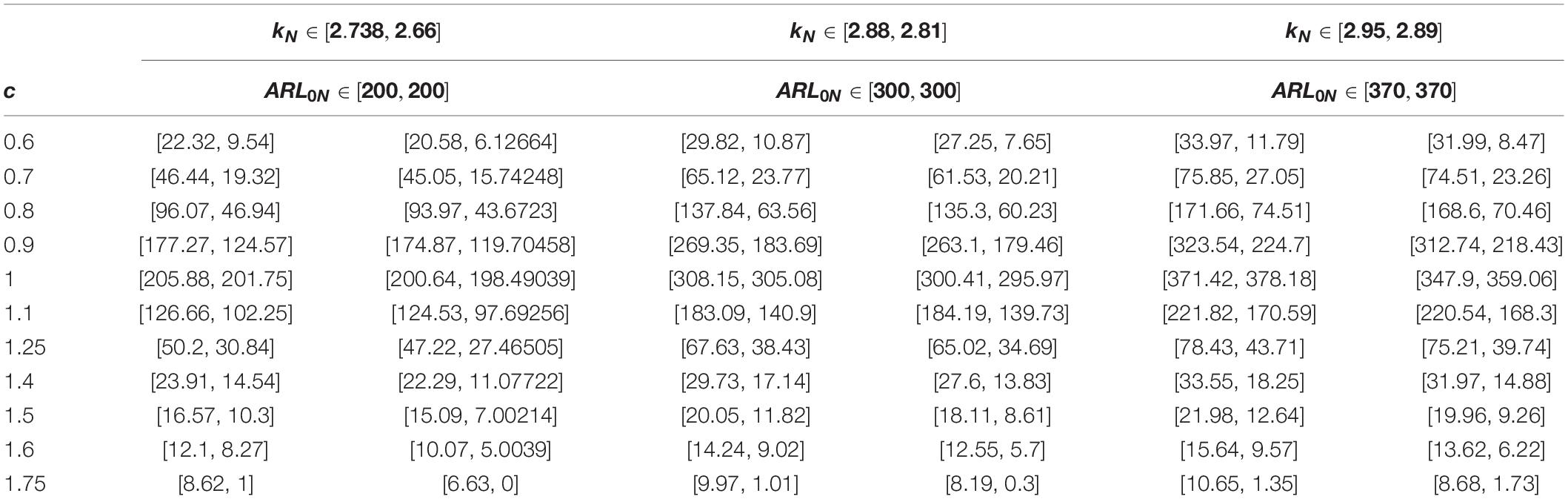
Table 1. The values of NARL when n_N ∈ [4,6] and w_N ∈ [3,5].

TABLE 2

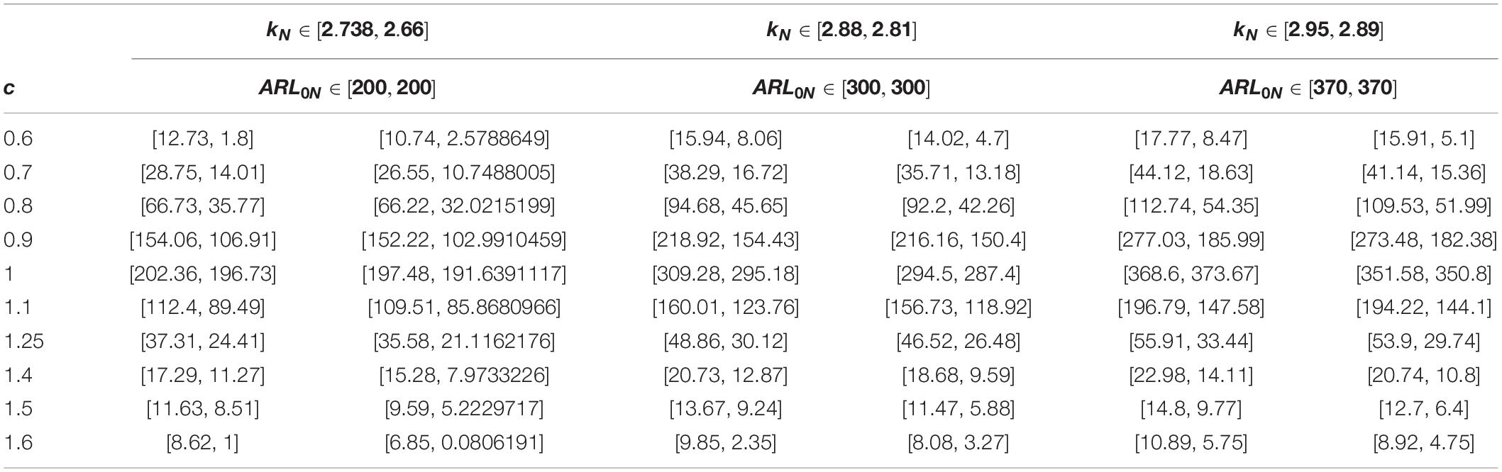
Table 2. The values of NARL when n_N ∈ [6,8] and w_N ∈ [3,5].

TABLE 3

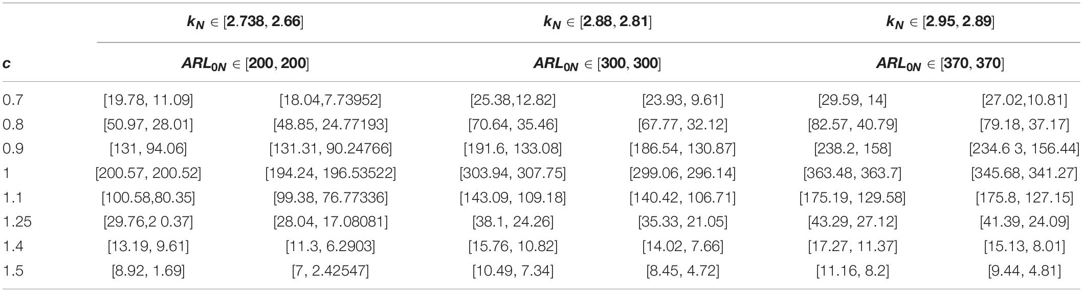
Table 3. The values of NARL when n_N ∈ [8,10] and w_N ∈ [3,5].

TABLE 4

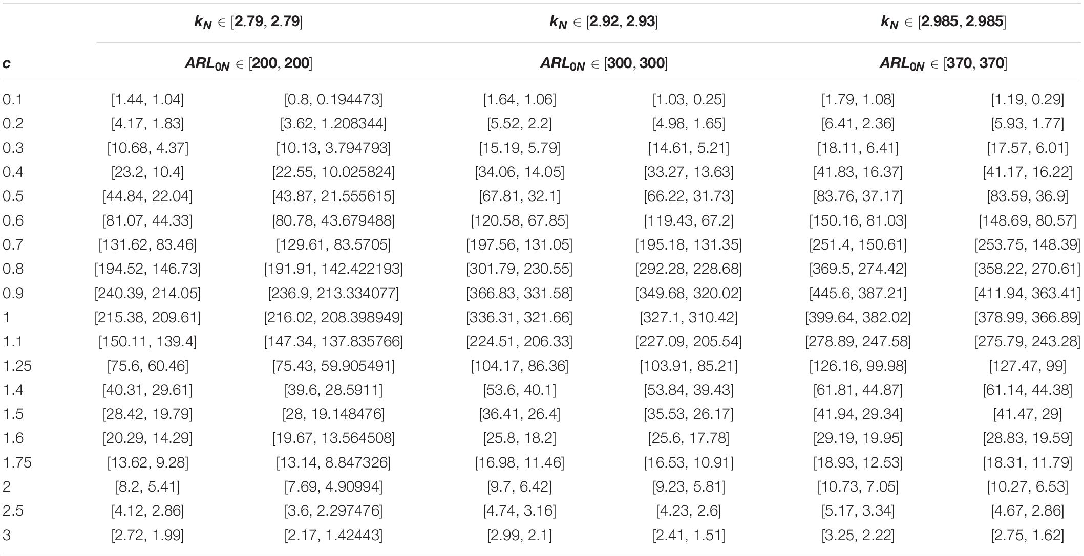
Table 4. The values of NARL when n_N ∈ [4,6] and w_N ∈ [1,1].

From Tables 1–4, the following trends are noted in ARL_1N ∈ [ARL_1L,ARL_1U]:

1. The values of k_N = k + E_NI_N; I_N ∈ [I_L,I_U] increase when r_0N ∈ [r_0L,r_0U] increases. For example, when r_0N ∈ [370,370], we note the maximum value of k_N = 2.95−2.89I_N; I_N ∈ [0,0.2076] in Table 1.

2. We note the decreasing trend in the indeterminacy interval of ARL_1N = ARL_L + ARL_UI_N; I_N ∈ [I_L,I_U] as n_N ∈ [n_L,n_U] increased and w_N = w_L + w_UI_N; I_N ∈ [I_L,I_U] is fixed. For example, when w_N = 3 + 5I_N; I_N ∈ [0,0.4] and c = 1.5, the value of ARL_1N is ARL_1N = 16.57−10.3I_N; I_N ∈ [0,0.6087], which is ARL_1N ∈ [16.57,10.3] when n_N ∈ [4,6]. When w_N = 3 + 5I_N; I_N ∈ [0,0.4] and c = 1.5, the value of ARL_1N is ARL_1N = 11.63−8.51I_N; I_N ∈ [0,0.3666], which is ARL_1N ∈ [11.63,8.51] when n_N ∈ [6,8].

3. We note the decreasing trend of measure of indeterminacy as n_N ∈ [n_L,n_U] increases.

Comparative Study

In this section, we compare the performance of the proposed NMA control chart with the proposed neutrosophic control chart for the exponential distribution and control chart under classical statistics in terms of NARL. The proposed NMA control chart is the extension of the proposed neutrosophic control chart for the exponential distribution and control chart for the exponential distribution under NS. The proposed NMA chart reduces to the proposed neutrosophic control chart for the exponential distribution when w_N ∈ [1,1]. Similarly, the proposed NMA chart reduces to Santiago and Smith (7) control chart when w_N ∈ [1,1] and I_L 0. In sections The Proposed NMA Chart vs. Proposed Neutrosophic Control Chart for the Exponential Distribution and “The Proposed Charts vs. Control Chart for the Exponential Distribution Under Classical Statistics”, we present the comparisons of the charts in terms of NARL. In section “Comparisons by Simulation,” we compare the charts using the simulated data.

The Proposed Neutrosophic MA Chart vs. Proposed Neutrosophic Control Chart for the Exponential Distribution

For a fair comparison between the proposed control charts, we set the same values of the control chart parameters. Tables 1–3 are shown for the proposed NMA chart, and Table 4 presents the proposed neutrosophic control chart for the exponential distribution. By comparing the values of ARL_1N = ARL_L + ARL_UI_N; I_N ∈ [I_L,I_U] presented in Table 4 with Table 1, we note that the proposed NMA chart has smaller values of ARL_1N = ARL_L + ARL_UI_N; I_N ∈ [I_L,I_U] at all shifts c. For example, when c = 1.5, the value of the indeterminacy interval of ARL_1N ∈ [ARL_1L,ARL_1U] is ARL_1N ∈ [19.96,9.26] from the proposed NMA chart. On the other hand, the value of the indeterminacy interval of ARL_1N ∈ [ARL_1L,ARL_1U] is ARL_1N ∈ [41.47,29] from the proposed NMA chart. From the values of ARL_1N ∈ [ARL_1L,ARL_1U], it is quite clear that the proposed NMA provides the smaller values of ARL_1N ∈ [ARL_1L,ARL_1U] as compared to the proposed neutrosophic chart for the exponential distribution. From this comparison, it can be noted that the proposed chart detects a shift in the process between the 9th and 19th samples, whereas the other proposed control chart detects a shift between the 29th and 41st samples. Therefore, the proposed NMA chart is more efficient in detecting the shift in the process as compared to the proposed exponential chart under NS.

The Proposed Charts vs. Control Chart for the Exponential Distribution Under Classical Statistics

We now compare the efficiency of the proposed control chart under NS with the control chart for the exponential distribution under classical statistics. Note here that the first values of the indeterminacy interval of ARL_1N = ARL_L + ARL_UI_N;I_N ∈ [I_L,I_U] in Tables 1–4 represent the average run length (ARL) of the chart under classical statistics. According to the theory of the proposed charts, the proposed charts reduces their competitive chart under classical statistics when I_N ∈ [0,I_U]. From Tables 1–4, it is quite obvious that the proposed control charts provide the smaller values of indeterminacy interval of ARL_1N = ARL_L + ARL_UI_N;I_N ∈ [I_L,I_U] as compared to the chart proposed by Santiago and Smith (7). For example, when c 1.1, the value of ARL from Santiago and Smith (7) chart is 275 and from the proposed chart it is 79. It means, that the existing chart tells about the shift in the process at the 275th sample, whereas the proposed chart tells that the shift can be detected between the 79th and 275th samples. From these comparisons, we conclude that the proposed control charts are flexible, informative, and passable to apply under uncertainty environment.

Comparisons by Simulation

To compare the performance of the three charts, we simulated the data from the NED. For the simulation study, let c 1.4, n_N ∈ [4,6], and ARL_1N ∈ [370,370]. The first 20 observations are generated from the in-control process, and the next 20 observations are generated from the shifted process when c 1.4. The values of NS MA_iN = MA_i + D_NI_N; I_N ∈ [I_L,I_U] are calculated and plotted on the three control charts in Figure 1. For these parameters, the tabulated NARL is [33.55, 18.25]. From Figure 1, it can be seen that the proposed control NMA (left in Figure 1) detects the shift at around the 25th sample. The proposed neutrosophic chart for the exponential distribution (middle chart) shows the shift at around the 35th sample, whereas the chart proposed by Santiago and Smith (7) does not show any shift in the process. From this comparison, it can be noted that the proposed chart has the ability to detect the shift in the process early than the proposed neutrosophic chart for the exponential distribution and chart proposed by Santiago and Smith (7).

FIGURE 1

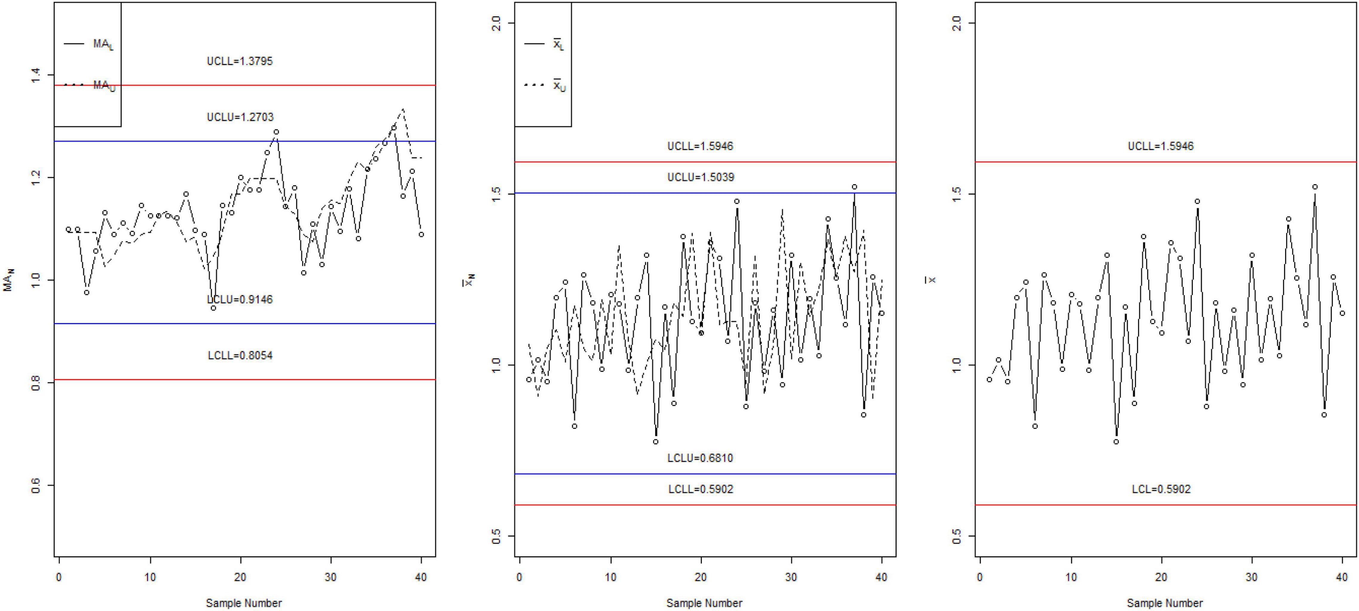
Figure 1. The control charts for simulated data.

Application of Proposed Chart Using Betaine Data

The application of the proposed chart is given using Betaine data. According to Mahmood et al. (41), “Betaine was introduced in artificial rumen containing ruminal fluid of cows. The objective was to determine the rate of disappearance of Betaine from incubation fluid at time points of 0, 1, 2, and 4 h after incubation and feeding of the system.” Note that the first four values are the original data taken from Mahmood et al. (41), and the next 20 observations of the data are generated from the exponential distribution with parameters [0.0042, 0.0076]. The data are shown in Table 5.

TABLE 5

Table 5. The Betaine data.

The values of NS MA_iN = MA_i + D_NI_N; I_N ∈ [I_L,I_U] are plotted on the proposed control chart and on the chart proposed by Santiago and Smith (7) as shown in Figure 2. From Figure 2, it is clear from the proposed control chart that although the control process is normal, some points are near the control limits, which need the Betaine process should be reviewed. On the other hand, using Betaine data, the control chart proposed by Santiago and Smith (7) indicates that the process is in the in-control state, and no action is needed. From this comparison, it is clear that the proposed chart indicates that some values denote indeterminate intervals and need attention.

FIGURE 2

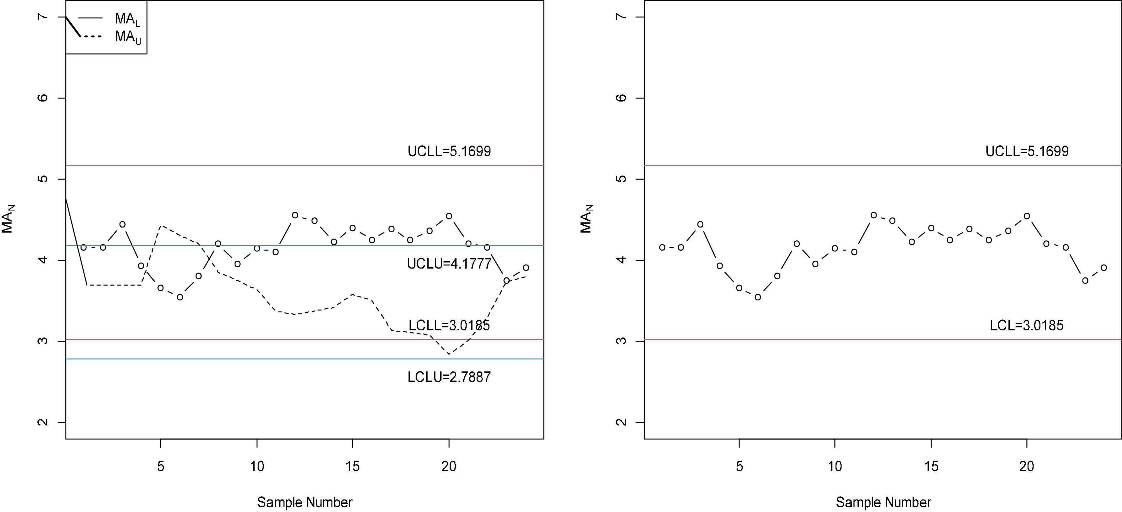
Figure 2. The proposed chart and the existing chart for Betaine data.

Concluding Remarks

A generalization of MA control chart for the exponential distribution under classical statistics is presented in this article. The designing of the MA control chart for the exponential distribution under NS is also presented. A Monte Carlo simulation under neutrosophic is introduced and applied to determine the neutrosophic control limits coefficients and NARL and neutrosophic standard deviation for various shifts. From the simulation study and real example, it is concluded that the proposed chart perform better than the competitors’ control chart in terms of NARL and NSD. The proposed chart is recommended when the practitioner is neutrosophic in sample size or span or observations or all. The proposed control chart using double sampling can be extended as future research.

Data Availability Statement

The original contributions presented in the study are included in the article/supplementary material, further inquiries can be directed to the corresponding author/s.

Author Contributions

MS, NK, and MA wrote the manuscript. All authors contributed to the article and approved the submitted version.

Funding

The work was supported by the Deanship of Scientific Research (DSR) at King Abdulaziz University; the authors, therefore, thank the DSR for their financial and technical support.

Conflict of Interest

The authors declare that the research was conducted in the absence of any commercial or financial relationships that could be construed as a potential conflict of interest.

Publisher’s Note

All claims expressed in this article are solely those of the authors and do not necessarily represent those of their affiliated organizations, or those of the publisher, the editors and the reviewers. Any product that may be evaluated in this article, or claim that may be made by its manufacturer, is not guaranteed or endorsed by the publisher.

Acknowledgments

We are deeply thankful to the editor and reviewers for their valuable suggestions to improve the quality and presentation of the article.

References

1. Derya K, Canan H. Control charts for skewed distributions: Weibull, gamma, and lognormal. Metodoloski Zvezki. (2012) 9:95. doi: 10.51936/ghaa8860

CrossRef Full Text | Google Scholar

2. Nelson PR. Control charts for Weibull processes with standards given. IEEE Trans Reliabil. (1979) 28:283–8. doi: 10.1109/TR.1979.5220605

CrossRef Full Text | Google Scholar

3. Bai D, Choi I. Over-bar-control and R-control charts for skewed populations. J Qual Technol. (1995) 27:120–31. doi: 10.1080/00224065.1995.11979575

CrossRef Full Text | Google Scholar

4. Zhang C, Xie M, Liu J, Goh T. A control chart for the gamma distribution as a model of time between events. Int J Prod Res. (2007) 45:5649–66. doi: 10.1080/00207540701325082

CrossRef Full Text | Google Scholar

5. Rahali D, Castagliola P, Taleb H, Khoo MB. Evaluation of Shewhart time-between-events-and-amplitude control charts for several distributions. Qual Eng. (2019) 31:240–54. doi: 10.1080/08982112.2018.1479036

CrossRef Full Text | Google Scholar

6. Choobineh F, Ballard J. Control-limits of QC Charts for skewed distributions using weighted-variance. IEEE Trans Reliabil. (1987) 36:473–7. doi: 10.1109/TR.1987.5222442

CrossRef Full Text | Google Scholar

7. Santiago E, Smith J. Control charts based on the exponential distribution: adapting runs rules for the t chart. Qual Eng. (2013) 25:85–96. doi: 10.1080/08982112.2012.740646

CrossRef Full Text | Google Scholar

8. Nelson LS. A control chart for parts-per-million nonconforming items. J Qual Technol. (1994) 26:239–40. doi: 10.1080/00224065.1994.11979529

CrossRef Full Text | Google Scholar

9. Aslam M, Khan N, Azam M, Jun C-H. Designing of a new monitoring t-chart using repetitive sampling. Inf Sci. (2014) 269:210–6. doi: 10.1016/j.ins.2014.01.022

CrossRef Full Text | Google Scholar

10. Aksoy H. Use of gamma distribution in hydrological analysis. Turk J Eng Environ Sci. (2000) 24:419–28.

Google Scholar

11. Borror CM, Keats JB, Montgomery DC. Robustness of the time between events CUSUM. Int J Prod Res. (2003) 41:3435–44. doi: 10.1080/0020754031000138321

CrossRef Full Text | Google Scholar

12. Chen Y-S, Yang Y-M. An extension of Banerjee and Rahim’s model for economic design of moving average control chart for a continuous flow process. Eur J Operat Res. (2002) 143:600–10. doi: 10.1016/S0377-2217(01)00341-1

CrossRef Full Text | Google Scholar

13. Wong H, Gan F, Chang T. Designs of moving average control chart. J Stat Comput Simul. (2004) 74:47–62. doi: 10.1080/0094965031000105890

CrossRef Full Text | Google Scholar

14. Khoo MB, Wong V. A double moving average control chart. Commun Stat Simul Comput. (2008) 37:1696–708. doi: 10.1080/03610910701832459

CrossRef Full Text | Google Scholar

15. Areepong Y. Optimal parameters of double moving average control chart. World Acad Sci Eng Technol Int J Math Comput Phys Electric Comput Eng. (2013) 7:1283–6.

Google Scholar

16. Mohsin M, Aslam M, Jun C-H. A new generally weighted moving average control chart based on Taguchi’s loss function to monitor process mean and dispersion. Proc Instit Mech Eng Part B J Eng Manufact. (2016) 230:1537–47. doi: 10.1177/0954405415625477

CrossRef Full Text | Google Scholar

17. Alghamdi SAD, Aslam M, Khan K, Jun C-H. A time truncated moving average chart for the Weibull distribution. IEEE Access. (2017) 5:7216–22. doi: 10.1109/ACCESS.2017.2697040

CrossRef Full Text | Google Scholar

18. Khademi M, Amirzadeh V. Fuzzy rules for fuzzy $ overline {X} $ and $ R $ control charts. Iran J Fuzzy Syst. (2014) 11:55–66.

Google Scholar

19. Intaramo R, Pongpullponsak A. Development of fuzzy extreme value theory control charts using α-cuts for skewed populations. Appl Math Sci. (2012) 6:5811–34.

Google Scholar

20. Faraz A, Moghadam MB. Fuzzy control chart a better alternative for Shewhart average chart. Qual Quant. (2007) 41:375–85. doi: 10.1007/s11135-006-9007-9

CrossRef Full Text | Google Scholar

21. Zarandi MF, Alaeddini A, Turksen I. A hybrid fuzzy adaptive sampling–run rules for Shewhart control charts. Inf Sci. (2008) 178:1152–70. doi: 10.1016/j.ins.2007.09.028

CrossRef Full Text | Google Scholar

22. Faraz A, Kazemzadeh RB, Moghadam MB, Bazdar A. Constructing a fuzzy Shewhart control chart for variables when uncertainty and randomness are combined. Qual Quant. (2010) 44:905–14. doi: 10.1007/s11135-009-9244-9

CrossRef Full Text | Google Scholar

23. Wang D, Hryniewicz O. A fuzzy nonparametric Shewhart chart based on the bootstrap approach. Int J Appl Math Comp Sci. (2015) 25:389–401. doi: 10.1515/amcs-2015-0030

CrossRef Full Text | Google Scholar

24. Kaya I, Erdoǧan M, YıldıZ C. Analysis and control of variability by using fuzzy individual control charts. Appl Soft Comput. (2017) 51:370–81. doi: 10.1016/j.asoc.2016.11.048

CrossRef Full Text | Google Scholar

25. Smarandache F. Introduction to Neutrosophic Statistics, Sitech and Education Publisher, Craiova. Columbus, OH: Romania-Educational Publisher (2014). p. 123.

Google Scholar

26. Chen J, Ye J, Du S. Scale effect and anisotropy analyzed for neutrosophic numbers of rock joint roughness coefficient based on neutrosophic statistics. Symmetry. (2017) 9:208. doi: 10.3390/sym9100208

CrossRef Full Text | Google Scholar

27. Chen J, Ye J, Du S, Yong R. Expressions of rock joint roughness coefficient using neutrosophic interval statistical numbers. Symmetry. (2017) 9:123. doi: 10.3390/sym9070123

CrossRef Full Text | Google Scholar

28. Aslam M, Khan N, Khan MZ. Monitoring the variability in the process using neutrosophic statistical interval method. Symmetry. (2018) 10:562. doi: 10.3390/sym10110562

CrossRef Full Text | Google Scholar

29. Aslam M. Design of sampling plan for exponential distribution under neutrosophic statistical interval method. IEEE Access. (2018) 6:64153–8. doi: 10.1109/ACCESS.2018.2877923

CrossRef Full Text | Google Scholar

30. Alhabib R, Ranna MM, Farah H, Salama A. Some neutrosophic probability distributions. Neutros Sets Syst. (2018) 22:30–8.

Google Scholar

31. Chutia R, Gogoi MK, Firozja MA, Smarandache F. Ordering single-valued neutrosophic numbers based on flexibility parameters and its reasonable properties. Int J Intell Syst. (2021) 36:1831–50. doi: 10.1002/int.22362

CrossRef Full Text | Google Scholar

32. Ye J. Bidirectional projection method for multiple attribute group decision making with neutrosophic numbers. Neural Comput Appl. (2017) 28:1021–9. doi: 10.1007/s00521-015-2123-5

CrossRef Full Text | Google Scholar

33. Ye J. Neutrosophic number linear programming method and its application under neutrosophic number environments. Soft Comput. (2018) 22:4639–46. doi: 10.1007/s00500-017-2646-z

CrossRef Full Text | Google Scholar

34. Ye J, Cui W, Lu Z. Neutrosophic number nonlinear programming problems and their general solution methods under neutrosophic number environments. Axioms. (2018) 7:13. doi: 10.3390/axioms7010013

CrossRef Full Text | Google Scholar

35. Mondal K, Pramanik S, Giri BC, Smarandache F. NN-Harmonic mean aggregation operators-based MCGDM strategy in a neutrosophic number environment. Axioms. (2018) 7:12. doi: 10.3390/axioms7010012

CrossRef Full Text | Google Scholar

36. Mondal K, Pramanik S, Giri BC. NN-TOPSIS strategy for MADM in neutrosophic number setting. Neutros Sets Syst. (2021) 47:66–92.

Google Scholar

37. Pramanik S, Banerjee D. Neutrosophic number goal programming for multi-objective linear programming problem in neutrosophic number environment. MOJ Curr Res Rev. (2018) 1:135–41. doi: 10.15406/mojcrr.2018.01.00021

CrossRef Full Text | Google Scholar

38. Maiti I, Mandal T, Pramanik S. Neutrosophic goal programming strategy for multi-level multi-objective linear programming problem. J Amb Intell Hum Comput. (2020) 11:3175–86. doi: 10.1007/s12652-019-01482-0

CrossRef Full Text | Google Scholar

39. Aslam M, Arif O. Testing of grouped product for the weibull distribution using neutrosophic statistics. Symmetry. (2018) 10:403. doi: 10.3390/sym10090403

CrossRef Full Text | Google Scholar

40. Montgomery DC. Introduction to Statistical Quality Control. Hoboken, NJ: John Wiley & Sons (2007).

Google Scholar

41. Mahmood M, Petri RM, Gavrãu A, Zebeli Q, Khiaosa-Ard R. Betaine addition as a potent ruminal fermentation modulator under hyperthermal and hyperosmotic conditions in vitro. J Sci Food Agric. (2020) 100:2261–71. doi: 10.1002/jsfa.10255

PubMed Abstract | CrossRef Full Text | Google Scholar