Liquidus curve of uranium–plutonium mixed oxide (MOX) system

Mixed oxides of uranium and plutonium (MOX) are currently considered reference fuels for the new generation of fast breeder reactors such as ASTRID. The key factor determining the performance and safety of fuel such as MOX is its operational limits in applied practice, which are closely related to the material’s structure and thermodynamic stability. They are, in turn, closely related to the ambient (zero pressure) melting point $(T_m)$; thus, $T_m$ is an important engineering parameter. However, the current knowledge of $T_m$ of MOX is limited and controversial, as several reported studies do not converge on the unique behavior of $T_m$ as a function of $x$. In this study, we present a theoretical model for the melting curve (liquidus) of a mixture and apply it to MOX considered a mixture of pure ${\text{UO}}_2$ and ${\text{PuO}}_2$. The model uses the known melting curves of pure constituents as an input and predicts the melting curve of their mixture. It has only one free parameter, which must be determined independently. In the case of MOX, $T_m$ of MOX as a function of $x$ as given by the model has a local minimum at $x\approx 0.64$, which disagrees slightly with our previous ab initio molecular dynamics studies that place this minimum at $x=0.7$.

1 Introduction

Nuclear power seems to be one of the most reliable energy sources for achieving the goal of a world free of man-made ${\text{CO}}_2$ emissions (Shellenberger, 2018). However, nuclear power has always been scrutinized for its potential impact on the environment and the safety issues related to its use (arising from accidents such as Chernobyl or Fukushima). The choice between the two possible nuclear fuels, uranium and mixed oxide (MOX), to determine the most adequate nuclear fuel cycle for the world’s future power needs has been debated. MOX has the advantage of producing less intermediate- and high-level waste. In addition, MOX is planned to be the fuel for the new generation of fast breeder reactors such as ASTRID (Advanced Sodium Technological Reactor for Industrial Demonstration).

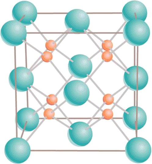
Uranium–plutonium MOX is the system ${\text{U}}_{1-x}$ ${\text{Pu}}_x$ ${\text{O}}_{2\pm y}$, where $x$ is the plutonium fraction; since the values of the atomic masses of U and Pu are very close (238 vs. 244), atomic and mass fractions virtually coincide, thus $x$ can be considered to be either of the two. Thus, $y=0$, $y>0$, and $y<0$ correspond to stoichiometric, hyperstoichiometric, and hypostoichiometric MOX, respectively. Both ${\text{UO}}_2$ and ${\text{PuO}}_2$ maintain their ambient cubic fluorite structure (Fm$\bar{3}$m) in the entire range of temperature $T$ up to the corresponding melting points. Specifically for ${\text{UO}}_2$, it is ($\rho$ is density, and $a$, $b$ and $c$ are unit cell dimensions) $\rho =10.97$ g/${\mathrm{c}\mathrm{m}}^3$, $a=b=c=5.47$ Å (Allen and Holmes, 1995), while for ${\text{PuO}}_2\rho =11.7$ g/${\mathrm{c}\mathrm{m}}^3$, $a=b=c=5.39$ Å (Wan et al., 2012). It is described in terms of a 12-atom unit cell containing four U (or Pu) atoms in face-centered cubic positions and eight O atoms filling the tetrahedral sites (Figure 1). Being a mixture of ${\text{UO}}_2$ and ${\mathrm{P}\mathrm{u}\mathrm{O}}_2$, MOX is also assumed to be of cubic fluorite structure at any $x$. With low Pu content $(x<0.1)$, it is used as nuclear fuel in several thermal neutron reactors around the world. With its higher Pu content, MOX is expected to be a favorable fuel for fast neutron reactors (FNRs). The constraint of the oxygen-to-metal (O/M, M = U + Pu) ratio less or equal to 2 is chosen as a safety precaution to protect the steel cladding from corrosion during irradiation in FNRs, even though this hypostoichiometry also has negative consequences such as inhomogeneity of Pu content, which may result in a reduced thermal conductivity of the MOX fuel.

Figure 1

Figure 1. Ambient fluorite structure of both ${\text{UO}}_2$ and ${\text{PuO}}_2$; uranium/plutonium atoms are shown in green and oxygen atoms in orange.

1.1 Ambient melting behavior

Of all the physical properties of a material, melting behavior is a fundamental property closely related to its structure and thermodynamic stability; it has thus always been a crucial subject of research. The ambient (zero pressure) melting point $(T_m)$ is also an important engineering parameter as it defines the operational limits of a material in its application environment. It becomes critical in nuclear engineering where the thermo-mechanical stability of a nuclear fuel element is a key factor in determining fuel performance and safety. Moreover, ${\text{PuO}}_2$ and ${\text{UO}}_2$ are two endpoints of the phase diagram of MOX, so their ambient $T_m$s are fundamental reference points.

The current knowledge of the $T_m$ of MOX is limited, and the literature does not converge on the unique behavior of $T_m$ as a function of $x$. Carbajo et al. (2001) and Guéneau et al. (2008) produced $T_m$ as a monotonically decreasing function of $x$ such that, with $T_m$ of ${\text{UO}}_2(x=0)$ of 3150 K, $T_m$ of ${\text{PuO}}_2(x=1)$ is $\sim 2650-2700$ K. However, the studies of Kato et al. (2008a), Kato et al. (2008b), De Bruyckner et al. (2010), and Böhler et al. (2014) resulted in $T_m$ having a local minimum at $0.5<x<1$ such that $T_m$ of ${\text{PuO}}_2$ is $\sim 3000-3050$ K so that the difference between the two values of $T_m$ is as high as 350 K. Although the melting behavior of uranium–plutonium MOX has been experimentally addressed in many recent studies, it still lacks a sound theoretical foundation. In particular, the melting behavior of MOX has not yet been adequately modeled based on general thermodynamics principles or using an equation of state (EOS) approach.

This uncertainty in the melting behavior of MOX is directly related to the ambiguity in the value of the ambient melting point of ${\text{PuO}}_2$ as well as the melting behavior of MOX with high Pu content. Since the 1960s, several research groups have reported measurements of $T_m$ of ${\text{PuO}}_2$ using various experimental techniques. Most are summarized in a review by Carbajo et al. (2001), who recommended a value of $2701\pm 35$ K based on measurements circa 1960s using the thermal arrest technique on tungsten-encapsulated samples. More recently, Guéneau et al. (2008) recommended a value of 2,660 K based on published data and the thermodynamic modeling of the Pu–O system. However, in the same year Kato and colleagues presented their experimental findings (Kato et al., 2008a; Kato et al., 2008b) which called into question the then commonly-accepted value of $T_m$ for ${\text{PuO}}_2$ and proposed a considerably higher value of $\sim 3000$ K. While using essentially the same thermal arrest technique as in the 1960s, Kato and colleagues paid particular attention to not only maintaining the exact O/M ratio as previous research had done but also to the effect of sample–crucible interactions. This way, they could attribute lower values of $T_m$ in previous studies to extensive interactions between ${\text{PuO}}_2$ samples and tungsten—typical crucible material in this range of $T$. The shortcomings thus indicated have been properly taken into account in the most recent experimental studies on the melting of ${\text{PuO}}_2$. These studies were carried out using a containerless laser-heating technique to produce values of $T_m$ for ${\text{PuO}}_2$: $3017\pm 28$ K (De Bruyckner et al., 2010) and $3050\pm 59$ K (Böhler et al., 2014). The most recent theoretical value of $T_m$ for ${\text{PuO}}_2$ is $3046\pm 135$ K (Burakovsky et al., 2023).

The difficulties with the experimental determinations of the melting behavior of the stoichiometric MOX as well as the shortcomings of the experimental techniques used for these determinations are summarized by Fouquet-Métivier et al. (2023) as follows. (i) The interaction of the ${\text{U}}_{1-x}{\text{Pu}}_x{\text{O}}_2$ samples of high Pu content with tungsten crucibles, and in some $x>0.5$ cases with rhenium crucibles, drives the corresponding $T_m$ systematically lower. (ii) Pu content affects the $T_m$ measurements such that laser heating, which is currently the most widely used technique, causes non-ideal behavior of the ${\text{UO}}_2$ and ${\text{PuO}}_2$ partitions of MOX, resulting in a distinct minimum of $T_m$ as a function of $x$ at $0.4<x<0.8$. (iii) The measured values of $T_m$ are affected by the O/M ratio, which varies in the atmosphere during the experiments so that it is not clear whether the measured $T_m$ corresponds to O/M close to 2 of the stoichiometric case or if it is much less than 2.

Hence, the clarification of the behavior of $T_m$ as a function of $x$ requires further study. Here, we present a theoretical model for the melting curve (liquidus) of a mixture and apply it to MOX which is considered a mixture of pure ${\text{UO}}_2$ and ${\text{PuO}}_2$.

2 Theoretical model for melting curve (liquidus) of a mixture

Here, we present a theoretical model for the melting curve of a mixture of two constituents. Such a mixture can be a compound or an alloy; even a porous material can be considered a mixture of a regular substance with air. Our approach can be easily generalized for a mixture of any number of constituents.

2.1 Preliminary considerations

We consider the case of ideal mixing, where the constituents of the mixture do not effectively interact with each other, which would otherwise result in the volume of the mixture being different from the sum of the volumes of its constituents. We assume that the mixture is of the form $A_{1-x}{B}_x$ and $0\le x\le 1$ and that no stoichiometric $A_n{B}_m$ (both $m$ and $n$ are integers $\ge 1$) compound exists; otherwise, additional arguments should be invoked regarding the enthalpy of formation of such a compound, which will result in a modification of the analytic form of the melting curve which we now derive. Thus, any eutectic is neglected. Our derivation is based on the assumption that both of the melting curves of pure constituents are known in the analytic form of the pressure $(P)$ dependence of the melting point: $T_m=T_m(P)$. This form can be either a simple polynomial fit, such as a quadratic or cubic, or a more sophisticated Simon–Glatzel form $T_m(P)=T_m(0){(1+P/a)}^b$, where $T_m(0)$ is the ambient $T_m$ and $a,b=\mathrm{c}\mathrm{o}\mathrm{n}\mathrm{s}\mathrm{t}$, etc. However, nothing else is known about the mixture, except the two melting curves; for example, their EOSs are not available. Thus, the model will predict the melting curve of a mixture based on the melting curves of its components only. Finally, we assume that both constituents of the mixture are molten and are in a state of thermal equilibrium with each other at a common temperature $T_m$ so that the two partial pressures are such that

$T_m^1\left(P_1\right)=T_m^2\left(P_2\right)=T_m.(1)$

In Equation 1 $T_m^1(P)$ and $T_m^2(P)$ are the melting curves of constituents 1 and 2, respectively, and $P_1$ and $P_2$ are the corresponding partial pressures at $T=T_m$. We thus model the system’s liquidus, which is the true melting line along which all the constituents are molten; our approach generally applies to systems, the constituents of which are not completely miscible so that the system’s phase diagram may have a miscibility gap. Thus, in what follows, we use the subscript $\ell$ instead of $m$ in order to associate the melting point with liquidus and not confuse it with solidus.

First, we develop the appropriate mixing rules. We begin with the EOS. If the cold $(T=0)$ EOSs of constituents 1 and 2 are, respectively, $P_1(\rho )$ and $P_2(\rho )$, their finite-$T$ counterparts can be written as

$P_1\left(\rho ,T\right)=P_1\left(\rho ,0\right)+{\alpha }_1{B}_{T,1}T,P_2\left(\rho ,T\right)=P_2\left(\rho ,0\right)+{\alpha }_2{B}_{T,2}T,(2)$

where $\alpha$ and $B_T$ are, respectively, the thermal expansion coefficient and isothermal bulk modulus at temperature $T$. This form of the thermal EOS does not explicitly take into account the $T$-dependence of the bulk modulus, and/or the $P$- (or $T$-) dependence of the thermal expansivity, and is therefore approximate. Indeed, since

$P\left(T,V\right)=P\left(T_0,V\right)+{\int }_{T_0}^T\alpha B_{T}dT,$

Equation 2 results from the above relation (with $T_0=0$) provided that $\alpha \cdot B_T\approx$ const—a potential weak $T$-dependence of $B$—is complemented by a similar weak dependence of $\alpha$ to keep their product (roughly) $T$-independent. As our previous theoretical studies reveal, thermal EOS of the form of Equation 2 holds for many substances, such as copper (Baty et al., 2021a), silver (Baty et al., 2021b), palladium (Baty et al., 2024), and body-centered cubic bismuth (Burakovsky et al., 2024a), among others. In fact, along the corresponding melting curves, thermal EOS of the form Equation 2 is virtually exact.

We use the pressure mixing rule (law of additive volumes, or the Amagat–Leduc model) which requires that the pressures of the components be equal at a chosen mixture composition, total volume, and temperature. This pressure mixing rule thus describes the pressure equilibrium of the mixture. The set of the equations that describe the mixture at pressure equilibrium are

$P_1\left({\rho }_1,T\right)=P_2\left({\rho }_2,T\right)(3)$

and

$\frac{1-x}{{\rho }_1}+\frac{x}{{\rho }_2}=\frac{1}{\rho }.(4)$

where ${\rho }_1$ and ${\rho }_2$ are, respectively, the densities of constituents 1 and 2, $\rho$ is the density of the mixture, and $x$ is the (fractional) mass percentage of constituent 2 (without any loss of generality we consider constituent 1 as a host and constituent 2 as a dopant): $x=M_2/(M_1+M_2)$, $1-x=M_1/(M_1+M_2)$. Equation 4 is equivalent to $M_1/{\rho }_1+M_2/{\rho }_2=(M_1+M_2)/\rho$, which is the total volume of the mixture being the sum of the volumes of its constituents. It follows from the above relation that

$\rho =\frac{{\rho }_1{\rho }_2}{x{\rho }_1+\left(1-x\right){\rho }_2}=\frac{\left(1-x\right){\rho }_1+x{\rho }_2}{1+\left(1-x\right)x\frac{{\left({\rho }_1-{\rho }_2\right)}^2}{{\rho }_1{\rho }_2}}.$

Hence, provided that $|{\rho }_1-{\rho }_2|\ll {\rho }_1,{\rho }_2$, the density of the mixture is quasi-additive: $\rho \approx (1-x){\rho }_1+x{\rho }_2$. This is the case for MOX since the values of the densities of pure ${\text{UO}}_2$ and ${\mathrm{P}\mathrm{u}\mathrm{O}}_2$, $\approx 10.97$ and 11.46 g/${\mathrm{c}\mathrm{m}}^3$, respectively (Carbajo et al., 2001), are indeed very close, and the density of ${\text{U}}_{1-x}{\text{Pu}}_x{\text{O}}_{2\pm y}$ is described by $\rho (x,y)=(10.97+0.49x)(1+0.0039y)$ (Carbajo et al., 2001). Here $x$ can be either mass or atomic (or volume) percentage discussed below because, for MOX, the two are essentially identical.

Note that in Equation 3 the value of $T$ cannot be arbitrarily high—that is, the range of $T$ for the applicability of the pressure mixing rule is limited. Indeed, at the liquidus temperature $T_{\text{ell}}$ all the constituents of the mixture are molten; hence, each individual $P$ is determined by the corresponding melting curve $T_m=T_m(P)$ such that, for constituent $i$, $T_{\text{ell}}=T_m^i(P^i(T_{\text{ell}}))$. Since different constituents have different melting curves $T_m^i=T_m^i(P)$, the corresponding values of $P^i(T_{\text{ell}})$ are different as well. Then, at $T=T_{\text{ell}}$ the value of $P$ of the mixture is generally not equal to any of the $P^i(T_{\text{ell}})$s and is given by a mixing rule different from Equations 3 and 4. This new mixing rule is discussed in more detail in the next section, taking into account that at the liquidus point, the mixture is at temperature rather than pressure equilibrium.

By switching from mass percentage $x$ to (atomic) volume percentage $X$, via

$X=\frac{x}{x+\left(1-x\right)\frac{m_2}{m_1}},1-X=\frac{1-x}{1-x+x\frac{m_1}{m_2}}.(5)$

In Equation 5 $m_1$ and $m_2$ are the atomic masses, respectively (hence $x=\frac{X}{X+(1-X)\frac{m_1}{m_2}}$ and $1-x=\frac{1-X}{1-X+X\frac{m_2}{m_1}})$, Equation 4 converts to

$v=\left(1-X\right)v_1+X{v}_2,(6)$

where $v$, $v_1$, and $v_2$ are the atomic volumes of the mixture and its constituent. Here, we define the atomic mass of the mixture as $m=(1-X)m_1+X{m}_2$. Equation 6 represents Zen’s law of the additivity of the atomic volume of a mixture (Zen, 1956) (analogous to the quasi-additivity of the density of the mixture discussed above). We note that in the case of real mixing, formulas for the total volume $\mathcal{V}={\mathcal{V}}_1+{\mathcal{V}}_2$ (resulting from Equation 4), or its atomic-volume analog Equation 6 must be replaced with, respectively, $\mathcal{V}={\tilde{\mathcal{V}}}_1+{\tilde{\mathcal{V}}}_2$ and $v=(1-X){\tilde{v}}_1+X{\tilde{v}}_2$. Here, “$\sim$” indicates the partial (effective) volume in the mixture, which may be larger or smaller than that in the ideal (non-interactive) case depending on whether the mixture constituents effectively attract or repel each other. It can be shown that in this case $v=(1-X)v_1+X{v}_2+(1-X)X{v}_{\text{def}}$, where $v_{\text{def}}$ is the defect of the volume additivity of the ideal-mixing case; here $v_{\text{def}}$ itself may be a function of $X$. Our model can in principle be formulated in the case of non-ideal mixing, but such a formulation would go well beyond the scope of our present work.

Since at fixed $T$, $P=-dE/dV$, the analog of the pressure mixing rule Equations 3, 4 for energy is

$E\left(\rho ,T\right)=\left(1-X\right)E_1\left({\rho }_1,T\right)+X{E}_2\left({\rho }_2,T\right).(7)$

In Equation 7 $E$, $E_1$, and $E_2$ are the energies of the mixture and its constituents. Here, $E_1(\rho ,T)$ and $E_2(\rho ,T)$ are directly related to, respectively, $P_1(\rho ,T)$ and $P_2(\rho ,T)$.

The “specific” Gibbs function—that is, the Gibbs function per unit mass which is consistent with the pressure mixing rule—is

$G=\left(1-x\right)G_1+x{G}_2.(8)$

Indeed, the specific volume of the mixture $(\sim 1/\rho )$ is $V={(\partial G/\partial P)}_T\equiv G_P=(1-x)V_1+x{V}_2$, which is equivalent to Equation 4. We note that, although this formulation is not conventional, it can be found in the literature, such as in Duvall and Taylor (1971), where it was used for the description of the shock compression of a two-component mixture. It then follows from Equation 8 that the specific entropy of the mixture is $S=-{(\partial G/\partial T)}_P\equiv -G_T=(1-x)S_1+x{S}_2$. The isothermal compressibility $(1/B_T)$ is $\beta =-(1/V){(\partial V/\partial P)}_T\equiv -G_{PP}/V$; hence, $\beta V=(1-x){\beta }_1{V}_1+x{\beta }_2{V}_2$. That is,

$\frac{1}{\rho B_T}=\frac{1-x}{{\rho }_1{B}_{T,1}}+\frac{x}{{\rho }_2{B}_{T,2}}.(9)$

Note that Equation 9 follows directly from Equation 4 written as the total volume of the system being the sum of the volumes of its constituents: $\mathcal{V}={\mathcal{V}}_1+{\mathcal{V}}_2$. Then, under a small pressure change of $\mathrm{\Delta }P$, the total volume change is $\mathrm{\Delta }\mathcal{V}=\mathrm{\Delta }{\mathcal{V}}_1+\mathrm{\Delta }{\mathcal{V}}_2$; therefore, since $B_T\equiv -\mathcal{V}{(\partial P/\partial \mathcal{V})}_T$, $B_{T,1}\equiv -{\mathcal{V}}_1{(\partial P/\partial {\mathcal{V}}_1)}_T$ and $B_{T,2}\equiv -{\mathcal{V}}_2{(\partial P/\partial {\mathcal{V}}_2)}_T$,

$\frac{\mathcal{V}}{B_T}=-\frac{\mathrm{\Delta }\mathcal{V}}{\mathrm{\Delta }P}=-\left(\frac{\mathrm{\Delta }{\mathcal{V}}_1}{\mathrm{\Delta }P}+\frac{\mathrm{\Delta }{\mathcal{V}}_2}{\mathrm{\Delta }P}\right)=\frac{{\mathcal{V}}_1}{B_{T,1}}+\frac{{\mathcal{V}}_2}{B_{T,2}}.(10)$

Equation 10 is equivalent to Equation 9 in view of Equation 4. We will also need the thermal expansion coefficient, $\alpha =(1/V){(\partial V/\partial T)}_P\equiv G_{PT}/V$ or $\alpha V=(1-x){\alpha }_1{V}_1+x{\alpha }_2{V}_2$, which is equivalent to

$\frac{\alpha }{\rho }=\frac{\left(1-x\right){\alpha }_1}{{\rho }_1}+\frac{x{\alpha }_2}{{\rho }_2}.(11)$

Now, dividing Equation 11 by Equation 9, upon some algebra, we arrive at

$\alpha B_T=\left(1-x\right){\alpha }_1{B}_{T,1}+x{\alpha }_2{B}_{T,2}+\left(1-x\right)x\left({\alpha }_1{B}_{T,1}-{\alpha }_2{B}_{T,2}\right)\left(\frac{\rho B_T}{{\rho }_1{B}_{T,1}}-\frac{\rho B_T}{{\rho }_2{B}_{T,2}}\right).$

Note that Equation 9 allows the following parametrization:

${\rho }_1{B}_{T,1}=\frac{\rho B_T}{1\pm Cx},{\rho }_2{B}_{T,2}=\frac{\rho B_T}{1\mp C\left(1-x\right)},(12)$

where $C$ is assumed to be a constant such that, regardless of the value of $C$, Equation 9 holds true because of the identity $(1-x)(1\pm Cx)+x(1\mp C(1-x))=1$. In the following, we keep the upper sign in front of $C$ in the two denominators of Equation 12 so that $C$ itself can be of either sign (or zero). We consider $C$ as the only free parameter of this formulation, the value of which must be determined independently—based on the available experimental information on the liquidus of the system. We assume that no other experimental information is available; in particular, on the values of $\rho B_T$, which would have otherwise allowed the calculation of the value of $C$ directly from Equation 12. Then, via Equation 12, $\rho B_T/({\rho }_1{B}_{T,1})-\rho B_T/({\rho }_2{B}_{T,2})=C$, which we use in the above relation for $\alpha B_T$ to finally obtain

$\alpha B_T=\left(1-x\right){\alpha }_1{B}_{T,1}+x{\alpha }_2{B}_{T,2}+\left(1-x\right)xC\left({\alpha }_1{B}_{T,1}-{\alpha }_2{B}_{T,2}\right).(13)$

2.2 The formula for the liquidus of a mixture

We now consider a two-component mixture at temperature equilibrium at the liquidus point $(P,T_{\ell })$ and assume that each of the components is described by thermal EOS of the form Equation 2. Then, for the pressures of the mixture and its components at $T=T_{\ell }$,

$P\left(\rho ,T_{\ell }\right)=P\left(\rho ,0\right)+\alpha B_T{T}_{\ell },P_1\left({\rho }_1,T_{\ell }\right)=P_1\left({\rho }_1,0\right)+{\alpha }_1{B}_{T,1}{T}_{\ell },P_2\left({\rho }_2,T_{\ell }\right)=P_2\left({\rho }_2,0\right)+{\alpha }_2{B}_{T,2}{T}_{\ell }.$

Since $P_1({\rho }_1,0)=P_2({\rho }_2,0)=P(\rho ,0)\equiv P$ (the pressure mixing rule), it then follows that ($P_{\ell ,1}\equiv P_1({\rho }_1,T_{\ell })$, $P_{\ell ,2}\equiv P_2({\rho }_2,T_{\ell })$, and $P_{\ell }\equiv P(\rho ,T_{\ell })$)

$\alpha B_T{T}_{\ell }=P_{\ell }-P,{\alpha }_1{B}_{T,1}{T}_{\ell }=P_{\ell ,1}-P,{\alpha }_2{B}_{T,2}{T}_{\ell }=P_{\ell ,2}-P,$

the use of which in Equation 13 multiplied by $T_{\ell }$, leading to

$P_{\ell }=\left(1-x\right)P_{\ell ,1}+x{P}_{\ell ,2}+\left(1-x\right)xC\left(P_{\ell ,1}-P_{\ell ,2}\right).(14)$

Equation 14 is our formula for the liquidus of a two-component mixture. It is in fact the new mixing rule mentioned above. Since both $P_{\ell ,1}=P_{\ell ,1}(T)$ and $P_{\ell ,2}=P_{\ell ,2}(T)$ are assumed to be available, provided that the value of $C$ is known, this formula gives the value of the melting $P$ of a mixture at any given melting temperature $T_{\ell }^{*}$ via $P_{\ell ,1}^{*}=P_{\ell ,1}(T_{\ell }^{*})$ and $P_{\ell ,2}^{*}=P_{\ell ,2}(T_{\ell }^{*})$.

2.3 General features of Eqs. (13) and (14)

It is important to note the general features of the above formulas for the product of $\alpha B_T$ and the liquidus of a mixture. Considering Equation 14 as a representative example, its general features are that it (i) is symmetrical under the simultaneous permutations $1\leftrightarrow 2$, $x\leftrightarrow (1-x)$, $C\leftrightarrow -C$, (ii) satisfies the boundary conditions $P_{\ell }(x=0)=P_{\ell ,1}$ and $P_{\ell }(x=1)=P_{\ell ,2}$, and (iii) satisfies the self-mixture condition where any pure substance can be considered a mixture with itself; hence, the choice of $P_{\ell ,1}=P_{\ell ,2}=\mathcal{P}$ should lead to $P_{\ell }=\mathcal{P}$ at any $x$. As clearly seen, this is achieved by the presence of $(P_{\ell ,1}-P_{\ell ,2})$ on the right-hand side of Equation 14.

3 Liquidus of a mixture at $P=0$ and small $P$

We note the above Formula 14 at $P=0$ and small $P$. In this case, both $T_{\ell ,1}(P)$ and $T_{\ell ,2}(P)$ can be approximated by simple linear forms:

$T_{\ell ,1}\left(P\right)=T_{\ell ,1}\left(0\right)+T_{\ell ,1}^{\prime }\cdot P,T_{\ell ,2}\left(P\right)=T_{\ell ,2}\left(0\right)+T_{\ell ,2}^{\prime }\cdot P,$

or $P_{\ell ,1}(T)=(T-T_{\ell ,1}(0))/T_{\ell ,1}^{\prime }(0)$, $P_{\ell ,2}(T)=(T-T_{\ell ,2}(0))/T_{\ell ,2}^{\prime }(0)$, where $T_{\ell ,1}(0)$, $T_{\ell ,2}(0)$, $T_{\ell ,1}^{\prime }(0)$, and $T_{\ell ,2}^{\prime }(0)$ are the corresponding ambient melting points and the initial slopes of the melting curves. Using these expressions in Equation 14 gives $T_{\ell }(P)=T_{\ell }(0)+T_{\ell }^{\prime }(0)\cdot P$, where

$T_{\ell }\left(0\right)=\frac{\frac{\left(1-x\right)T_{\ell ,1}\left(0\right)}{T_{\ell ,1}^{\prime }\left(0\right)}+\frac{x{T}_{\ell ,2}\left(0\right)}{T_{\ell ,2}^{\prime }\left(0\right)}+\left(1-x\right)xC\left(\frac{T_{\ell ,1}\left(0\right)}{T_{\ell ,1}^{\prime }\left(0\right)}-\frac{T_{\ell ,2}\left(0\right)}{T_{\ell ,2}^{\prime }\left(0\right)}\right)}{\frac{1-x}{T_{\ell ,1}^{\prime }\left(0\right)}+\frac{x}{T_{\ell ,2}^{\prime }\left(0\right)}+\left(1-x\right)xC\left(\frac{1}{T_{\ell ,1}^{\prime }\left(0\right)}-\frac{1}{T_{\ell ,2}^{\prime }\left(0\right)}\right)}(15)$

and

$\frac{1}{T_{\ell }^{\prime }\left(0\right)}=\frac{1-x}{T_{\ell ,1}^{\prime }\left(0\right)}+\frac{x}{T_{\ell ,2}^{\prime }\left(0\right)}+\left(1-x\right)xC\left(\frac{1}{T_{\ell ,1}^{\prime }\left(0\right)}-\frac{1}{T_{\ell ,2}^{\prime }\left(0\right)}\right).(16)$

These are expressions for the ambient melting point and initial slope of the melting curve of a mixture, respectively. Note that they both satisfy the self-mixture condition, again because of the presence of terms $\left(T_{\ell ,1}(0)/T_{\ell ,1}^{\prime }(0)-T_{\ell ,2}(0)/T_{\ell ,2}^{\prime }(0)\right)$ and $\left(1/T_{\ell ,1}^{\prime }(0)-1/T_{\ell ,2}^{\prime }(0)\right)$.

Thus, the analytical form of the liquidus of a mixture at small $P$ is

$T_{\ell }\left(P\right)=T_{\ell }\left(0\right)+T_{\ell }^{\prime }\left(0\right)\cdot P,$

where $T_{\ell }(0)$ and $T_{\ell }^{\prime }(0)$ are determined, respectively, by Equations 15 and 16.

3.1 General features of Eqs. (15) and (16)

Both $T_{\ell }(0)$ in Equation 15 and $T_{\ell }^{\prime }(0)$ in Equation 16 as functions of $x$ have a local extremum (either minimum or maximum) at

$\mathcal{X}=\frac{C-1}{2C}.(17)$

If this extremum does occur for the mixture, then $0<\mathcal{X}<1$, which puts a constraint on $C$: $|C|>1$, such that

$C>1\iff 0<\mathcal{X}<0.5,C<-1\iff 0.5<\mathcal{X}<1.(18)$

Equation 18 is consistent with the invariance under the simultaneous permutations $x\leftrightarrow (1-x)$ and $C\leftrightarrow -C$. In this case, the values of $T_m(0)$ and $T_m^{\prime }(0)$ at $x=\mathcal{X}$ are

$T_{\ell }^{\mathcal{X}}\left(0\right)=\frac{{\left(C-1\right)}^2{T}_{\ell ,1}^{\prime }\left(0\right)T_{\ell ,2}\left(0\right)-{\left(C+1\right)}^2{T}_{\ell ,2}^{\prime }\left(0\right)T_{\ell ,1}\left(0\right)}{{\left(C-1\right)}^2{T}_{\ell ,1}^{\prime }\left(0\right)-{\left(C+1\right)}^2{T}_{\ell ,2}^{\prime }\left(0\right)}(19)$

and

$T_{\ell }^{\prime \mathcal{X}}\left(0\right)=\frac{4C{T}_{\ell ,1}^{\prime }\left(0\right)T_{\ell ,2}^{\prime }\left(0\right)}{{\left(C-1\right)}^2{T}_{\ell ,1}^{\prime }\left(0\right)-{\left(C+1\right)}^2{T}_{\ell ,2}^{\prime }\left(0\right)}.(20)$

If, however, $|C|\le 1$, the extremum occurs either outside the physical region $0\le x\le 1$ of the mixture or at one of its endpoints (if $|C|=1$), both the local maximum and minimum are at the two endpoints, and $T_{\ell }(0)$ is a monotonically decreasing or increasing function of $x$. In this case, Equations 19, 20 do not apply.

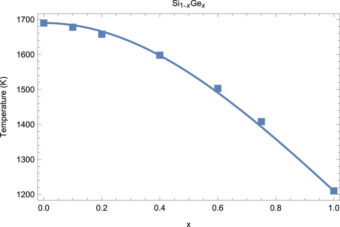
3.2 Example: Si–Ge system

Based on general considerations, it is expected that $C=\mathcal{O}(1)$. In the following example of the application of our model to a real system, $C$ is identically 1. The system that we are considering here is a mixture of silicon and germanium which, according to Olesinski and Abbaschian (1984), form a continuous solid solution without any eutectics. According to the literature (Jayaraman et al., 1963; Deb et al., 2001; Yang et al., 2004; Yang and Jiang, 2004; Kubo et al., 2008; Pasternak et al., 2008), the low-$P$ melting curves of Si and Ge are, respectively, $T_m^{\text{Si}}(P)=1690-63P$ and $T_m^{\text{Ge}}(P)=1210-50P$. Hence, this is an example of a mixture of “anomalous” melters, which both exhibit $T_m$ decreasing with $P$ (for the vast majority of substances, $T_m$ increases with $P$, which is the normal case). Hence, in Equation 15 $T_{\ell ,1}(0)=1690$, $T_{\ell ,1}^{\prime }(0)=-63$, $T_{\ell ,2}(0)=1210$, and $T_{\ell ,2}^{\prime }(0)=-50$. Then, the best fit of the form Equation 15 with the above parameters to the experimental data of Olesinski and Abbaschian (1984) brings up $C=1$. In Figure 2, the resulting $T_{\ell }(x)$ is compared to the liquidus of ${\text{Si}}_{1-x}{\text{Ge}}_x$ from the experiment.

Figure 2

Figure 2. Ambient phase diagram of the Si–Ge system: comparison of the liquidus curve produced by the theoretical model presented in this work to the experimental data points of Olesinski and Abbaschian (1984).

4 Application to the uranium–plutonium mixed oxide (MOX) system

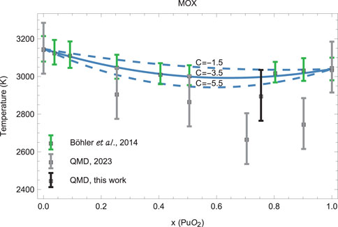
We now apply Formula 15 to the uranium–plutonium mixed oxide (MOX) system. Note that generally the value of $C$ can be determined from fitting $T_m(0)$ of the functional form Equation 15 to the experimental and/or theoretical data on the liquidus of a mixture. In the case of MOX, we determine the value of $C$ from fitting to the most recent and reliable experimental data (Böhler et al., 2014). We consider ${\text{UO}}_2$ as a host and ${\text{PuO}}_2$ as a dopant. The other parameter values required for the application of Equation 15 to MOX which we use for the determination of the values of $C$ are $T_{\ell ,1}(0)=3147$ K, $T_{\ell ,1}^{\prime }(0)=92.9$ K/GPa (Manara et al., 2010) and $T_{\ell ,2}(0)=3046$ K, $T_{\ell ,2}^{\prime }(0)=92.5$ K/GPa (Burakovsky et al., 2023). Taking into account the error bars of the experimental values of $T_{\ell }$, the fitting brings up the value of $C=-3.5\pm 2.0$, which we use in Equation 15. Then, in view of Equation 17 $\mathcal{X}\approx 0.64$, the local extremum (in our case, minimum) of the liquidus of MOX occurs at $x\approx 0.64$. This contrasts with our previous QMD studies which placed this minimum at $x=0.7$, although the difference is less than 10%.

Comparison of the liquidus of MOX in the form Equation 15 to both the experimental data of Böhler et al. (2014) and the results of our own ab initio quantum molecular dynamics (QMD) simulations is shown in Figure 3. The solid blue line corresponds to the model liquidus with $C=-3.5$, and the upper and lower dashed blue lines to, respectively, $C=-1.5$ and $C=-5.5$ which are the upper and lower limits of $C$. As Figure 3 clearly demonstrates, our model is in excellent agreement with the experiment, but there is some disagreement with the QMD data points for both $x=0.7$ and 0.9. We assume that the lower values of the two $T_m$s may be related to size effects in our QMD simulations. An example is the case of pure ${\text{UO}}_2$ (Burakovsky et al., 2024b), although the $T_m$ values for both smaller and larger systems are consistent within error bars. To test this assumption, we carried out QMD simulations to obtain another data point at $x=0.75$, this time using a 768-atom $(4\times 4\times 4)$ supercell, which is much larger than the 324-atom $(3\times 3\times 3)$ supercells used in our previous study.

Figure 3

Figure 3. Ambient phase diagram of stoichiometric MOX: comparison of the liquidus curve (blue lines) produced by the theoretical model presented in this work to both the experimental data points of Böhler et al. (2014) and the theoretical melting points from QMD simulations of our previous (2023) and current studies.

4.1 QMD simulations of the ambient $T_m$ of ${\mathrm{U}}_{0.25}{\text{Pu}}_{0.75}{\text{O}}_2$

The computational details of our QMD simulations can be found in our previous work on this subject (Burakovsky et al., 2023; Burakovsky et al., 2024b). The mixed ${\mathrm{U}\mathrm{O}}_2$-${\text{PuO}}_2$ system is modeled as a substitution alloy in which some U atoms (at randomly chosen lattice sites) are replaced by Pu atoms according to the corresponding ${\text{PuO}}_2$ content. Specifically, for our simulations of a 768-atom ${\text{U}}_{0.25}{\text{Pu}}_{0.75}{\text{O}}_2$ system, 576 U atoms chosen at random are replaced with 576 Pu atoms (alternatively, 192 Pu atoms of pure 768-atom ${\text{PuO}}_2$ systems are replaced with 192 U atoms chosen at random).

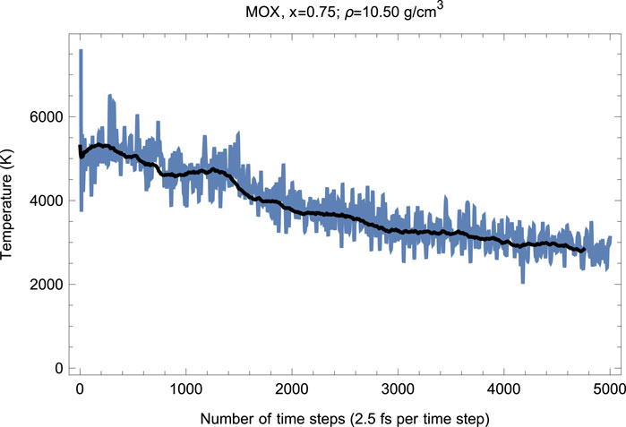
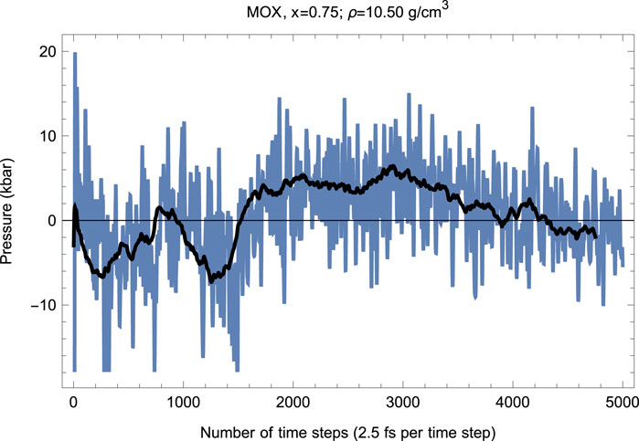
Our melting simulations are carried out using the so-called Z method (Burakovsky et al., 2015). In these simulations, the ${\text{U}}_{0.25}{\text{Pu}}_{0.75}{\text{O}}_2$ supercell is subject to a set of initial temperatures $(T_0)$ separated by an increment of 250 K and run with QMD in the $NVE$ ensemble, for a total of 5,000–6,000 time steps of 2.5 fs each—up to a total of 15 ps of running time—to determine $T_m$ at the corresponding melting pressure $(P_m)$. As the system equilibrates upon the completion of the melting process, the values of $T_m$ and $P_m$ are determined from the corresponding running averages (shown as solid lines in Figures 4 and 5). In this case, $P_m=0$ corresponds to the unit cell of $a=b=c=5.58$ Å or $\rho =10.50$ g/${\mathrm{c}\mathrm{m}}^3$.

Figure 4

Figure 4. Time evolution of temperature in the Fm$\bar{3}$m-${\text{UO}}_2$ melting run at $\rho =10.5$ g/${\mathrm{c}\mathrm{m}}^3$; initial temperature is 8500 K.

Figure 5

Figure 5. Same as in Figure 4 for the time evolution of pressure (in kbar; 10 kbar = 1 GPa).

As seen in Figures 4 and 5, since the beginning of the run, after $\sim 600$ time steps (1.5 ps), $T$ decreases and $P$ increases (since in the $NVE$ ensemble the total energy $E\sim k_{B}T+PV$ is conserved). This is a signature of a superionic transition. Due to a 15-fold difference in the atomic masses of U/Pu and O, the O sublattice becomes less stable than for U/Pu, and when sufficiently high $T$ it disorders first, such that the anions (${\text{O}}^{-}$) start flowing through the ordered structure of the cations (${\text{U}}^{+}$/${\mathrm{P}\mathrm{u}}^{+}$). Such a (superionic) phase transition accompanied by a rapid increase in ionic conductivity has been observed in many diatomic systems. It was observed in both pure ${\text{UO}}_2$ (Dworkin and Bredig, 1968) and ${\text{PuO}}_2$ (Chroneos et al., 2015; Günay et al., 2016). Figures 4 and 5 demonstrate its occurrence in ${\text{U}}_{0.25}{\text{Pu}}_{0.75}{\text{O}}_2$.

Thus, the first drop in $T$ (increase in $P$) corresponds to the activation of the O flow. This process takes $\sim 1000$ time steps ($\sim 2.5$ ps). The system of quasi-static cations and mobile anions then equilibrates, and the second drop in $T$ (increase in $P$) occurs after a total of $\sim 1400$ time steps ($\sim 3.5$ ps). This second drop in $T$ is associated with the disordering of the U/Pu sublattice—a true melting transition—and the corresponding $(P,T)$ point lies on the system’s liquidus. The melting process takes $\sim 600$ time steps (1.5 ps). The emerging liquid equilibrates at $(P,T)\approx (0,2900\mathrm{K})$, which is the liquidus point of ${\text{U}}_{0.25}{\text{Pu}}_{0.75}{\text{O}}_2$.

Hence, our ab initio ambient melting point of ${\text{U}}_{0.25}{\text{Pu}}_{0.75}{\text{O}}_2$ appears to be $2900\pm 135$ K. Uncertainty of the value of $T_m$ intrinsic to the Z method is 125 K, half of the increment of $T_0$ (Burakovsky et al., 2015), which turns out to constitute $\sim 4$% of $T_m$. Uncertainty of the value of $P_m$ in our simulations is $\sim 0.5$ GPa. Assuming that the initial slope of the melting curve ($d{T}_m/dP$ at $P$ = 0) is $\sim 90$ K/GPa, as predicted by the model (Equation 16), a $P_m$ uncertainty of 0.5 GPa translates into a $T_m$ uncertainty of $\delta T_m\sim \frac{d{T}_m}{dP}\delta P\stackrel{<}{\sim }45$ K. Therefore, the combined uncertainty of $T_m$ in our QMD simulations is $\approx 135$ K, which is within 5% of $T_m$. Thus, our results on the ambient $T_m$ of ${\text{U}}_{0.25}{\text{Pu}}_{0.75}{\text{O}}_2$ are expected to be quite accurate overall.

Our value of $T_m(0)=2900$ K for ${\text{U}}_{0.25}{\text{Pu}}_{0.75}{\text{O}}_2$ is $\sim 200$ K above the value of $\sim 2700$ K suggested by our previous QMD simulations of smaller systems (Burakovsky et al., 2023). Hence in our simulations, some size effects are indeed present and should therefore be taken into account. Assuming that the results on smaller supercells at $x=0.7$ and 0.9 should be corrected by adding $\sim 200$ K to the corresponding values of $T_m$s, the two corrected values would be fully consistent with the theoretical liquidus curve.

5 Discussion of the results

As Figure 3 clearly shows, the distinct minimum of $T_{\ell }=T_{\ell }(x)$ is at $x\approx 0.64$, as predicted by the model. We note that a very recent study of the MOX phase diagram using the Calphad methodology (Fouquet-Métivier et al., 2023) suggests the phase diagram of MOX (Figure 5 of Fouquet-Métivier et al., 2023) is very similar to our Figure 3, for which the liquidus line $T_{\ell }=T_{\ell }(x)$ has a distinct minimum at $x\approx 0.64$ and which is in good agreement with the experimental results by Böhler et al. (2014) rather than those of Kato et al. (2008a) and Lyon and Baily (1967) —just as the model liquidus curve on our MOX phase diagram is. Their value of $T_{\ell }\approx 2975$ K at $x=0.7$ is consistent with our value of $T_{\ell }=2993\pm 49$ at $x=0.64$ (as predicted by Equations 15 or 19 with $C=-3.5\pm 2.0$). One additional source of uncertainty of experimental measurements may be the variation of the O/M ratio during the melting of MOX in the atmosphere, which may contribute as much as $\sim 100$ K to the error in the experimental $T_{\ell }$ (Strach et al., 2016). Below, we discuss this point in more detail. Hence, the point we made previously (Burakovsky et al., 2023) that the two values of $T_{\ell }$ for MOX at $x=0.7$—that of Fouquet-Métivier et al. (2023) and $T_{\ell }=2670\pm 135$ K from our previous QMD studies which is $\sim 300$ K below—cannot be reconciled within the uncertainties of our method itself, is now resolved; the reason for this disagreement being size effects in our QMD simulations is clarified in our present study.

In Böhler et al. (2014), which was chosen for the construction of our theoretical model, the analysis of the experimental data on the melting of MOX revealed first that the congruent melting for the mixed oxides is shifted toward low O/M ratios compared to the end-members (${\text{UO}}_{1.97}$ and ${\text{PuO}}_{1.95}$). Second, the samples are highly oxidized in air whereas they are close to stoichiometry (O/M = 2.00) in the inert atmosphere of argon. This high oxidation results in hyperstoichiometry and may in principle lead to the formation of higher oxides such as ${\text{M}}_3{\text{O}}_8$ and/or ${\text{MO}}_3$. Both higher and lower O/M ratios may influence the values of $T_m$ which are used for both the determination of the value of $C$ and comparison to our theoretical results. While the literature generally agrees on the increase of $T_m$ for hyperstoichiometric MOX (e.g. Strach et al., 2016), some ambiguity persists regarding hypostoichiometric MOX. According to most studies, $T_m$ should decrease with decreasing O/M (e.g. Kato et al., 2008a; Kato et al., 2008b), just as it does with increasing O/M. However, several recent studies, both experimental (Morimoto et al., 2005; Kato et al., 2011) and theoretical using Calphad calculations (Guéneau et al., 2019; Fouquet-Métivier et al., 2020), have shown exactly the opposite. For example, Morimoto et al. (2005) focused on the dependence of $T_m$ of MOX with 30% Pu, 2% Am, and 2% Np on the deviation from stoichiometry, which indicates an unexpected decrease of $T_m$ toward O/M = 2. They concluded that the melting points of the pellets with O/M = 1.95 is higher than those with O/M = 1.98. Additionally, Calphad calculations reported in Guéneau et al. (2019) and Fouquet-Métivier et al. (2020) show a maximum $T_m$ around O/M = 1.98 rather than 2.00. These considerations must, however, consider the uncertainty on the fuel O/M ratio upon measurement due to the oxidation of the samples during the successive laser shots of the experimental procedure described in Fouquet-Métivier et al. (2020), which is around 2%, or 60 K, comparable to the $2\sigma$ uncertainty band of the experimental $T_m$ of Böhler et al. (2014). Because, as mentioned above, the uncertainty of $T_m$ associated with the combined effect of (i) deviation from stoichiometry, (ii) oxidation in air, and (iii) sample–crucible cross-contamination should be expected to be within $\sim 100$ K, the overall uncertainty of the most recent and accurate experiments on the melting of MOX is likely within $\sim 150$ K, which is essentially of the same magnitude as that of the Z method itself used for the QMD simulations of $T_m$. To summarize, the experimental data of Böhler et al. (2014) used to construct our theoretical model seem quite accurate overall; therefore, the model parameters, $C$ in particular, are reliable as well.

6 Concluding remarks

Our study presented a theoretical model for the melting curve (liquidus) of a mixture and applied it to the uranium–plutonium mixed oxide (MOX) system being considered a mixture of pure ${\text{UO}}_2$ and ${\text{PuO}}_2$.

The model is based on the two assumptions that (i) the mixture is ideal—that is, the additivity of the volumes of the constituents Equations 4 and 6 is realized—and (ii) the thermal EOS of each of the constituents as well as that of the mixture is given by Equation 2 in which $({\alpha }_1{B}_{T,1})$, $({\alpha }_2{B}_{T,2})$ and $(\alpha B_T)$ are all assumed to be constant. Their values are related by Equation 13 in which $C$ is the only free parameter that must be determined independently. We here discussed the way this is determined in practice. In addition to the melting curves of pure constituents (which are assumed to be available), no other experimental information is required as the model’s input. As regards the value of $C$, the example of MOX considered in our work clearly demonstrates that the variation of $C$ by as much as $\sim 60$% causes a shift of the model liquidus within $\sim 100$ K, or $\sim 3$%. In the case of ${\text{Si}}_{1-x}{\text{Ge}}_x$, a variation of $C$ of 60% would cause a shift of the model liquidus within $\sim 150$ K, or $\sim 10$%. Thus, the exact knowledge of the value of $C$ may not really be necessary for the model to produce the liquidus of a mixture in good agreement with the experiment.

The examples of the application of the model to real mixtures, Si–Ge and MOX, considered in our work clearly demonstrate that, although the model is not based on rigorous thermodynamic arguments, it is reliable and relatively easy to apply in practice, in contrast to more complicated and more time-consuming Calphad calculations.

Comparison of the MOX liquidus given by this model to experimental and QMD results is shown in Figure 3, which demonstrates very good agreement between the model and both experiment and theory. Figure 3 represents the current knowledge of the ambient phase diagram of stoichiometric MOX; this knowledge may be advanced further in subsequent studies on the subject.

Finally, we note that the present model can be further improved by taking into account the realistic scenario of the presence of a defect of the volume additivity, $v_{\text{def}}$ because of effective interactions between the constituents (Section 2.1) as well as a possible dependence of $C$ on $x$. As we have seen, taking $C$ in Equation 15 to be a constant results in a liquidus of a mixture in good (or even excellent, in the case of ${\text{Si}}_{1-x}{\text{Ge}}_x$) agreement with experiments; thus, the present model should be expected to predict reliable liquidi of different two-component mixtures. However, introducing a $x$-dependence of $C$ may help in addressing more exotic mixing cases, such as those in which eutectics are present. Of course, the generalization of the present model to mixtures of larger number of constituents (perhaps even an arbitrary number of them) will be undertaken in our subsequent research.

Data availability statement

The raw data supporting the conclusions of this article will be made available by the authors, without undue reservation.

Author contributions

LB: conceptualization, investigation, methodology, writing–original draft, and writing–review and editing. DP: conceptualization, investigation, methodology, supervision, and writing–review and editing. AG: funding acquisition, project administration, resources, supervision, and writing–review and editing.

Funding

The author(s) declare that financial support was received for the research, authorship, and/or publication of this article. This research was carried out under the auspices of the US DOE/NNSA.

Acknowledgments

The work was done under the auspices of the US DOE/NNSA. The QMD simulations have been performed on the LANL cluster Chicoma as part of the Institutional Computing project ${\text{w}24}_{-}$phadiagractox.

Conflict of interest

The authors declare that the research was conducted in the absence of any commercial or financial relationships that could be construed as a potential conflict of interest.

Publisher’s note

All claims expressed in this article are solely those of the authors and do not necessarily represent those of their affiliated organizations, or those of the publisher, the editors, and the reviewers. Any product that may be evaluated in this article, or claim that may be made by its manufacturer, is not guaranteed or endorsed by the publisher.

References

Allen, G. C., and Holmes, N. R. (1995). A mechanism for the UO₂ to α-U₃O₈ phase transformation. J. Nucl. Mater. 223, 231–237. doi:10.1016/0022-3115(95)00025-9

CrossRef Full Text | Google Scholar

Baty, S. R., Burakovsky, L., and Errandonea, D. (2021a). Ab initio phase diagram of copper. Crystals 11, 537. doi:10.3390/cryst11050537

CrossRef Full Text | Google Scholar

Baty, S. R., Burakovsky, L., and Errandonea, D. (2021b). Ab initio phase diagram of silver. J. Phys. Condens. Matter 33, 485901. doi:10.1088/1361-648x/ac23fb

PubMed Abstract | CrossRef Full Text | Google Scholar

Baty, S. R., Burakovsky, L., Luscher, D. J., Anzellini, S., and Errandonea, D. (2024). Palladium at high pressure and high temperature: a combined experimental and theoretical study. J. Appl. Phys. 135, 075103. doi:10.1063/5.0179469

CrossRef Full Text | Google Scholar

Böhler, R., Welland, M., Prieur, D., Cakir, P., Vitova, T., Pruessmann, T., et al. (2014). Recent advances in the study of the UO₂–PuO₂ phase diagram at high temperatures. J. Nucl. Mater. 448, 330–339. doi:10.1016/j.jnucmat.2014.02.029

CrossRef Full Text | Google Scholar

Burakovsky, L., Burakovsky, N., and Preston, D. L. (2015). Ab initio melting curve of osmium. Phys. Rev. B 92, 174105. doi:10.1103/physrevb.92.174105

CrossRef Full Text | Google Scholar

Burakovsky, L., Ramsey, S. D., and Baty, R. S. (2023). Ambient melting behavior of stoichiometric uranium-plutonium mixed oxide fuel. Appl. Sci. 13, 6303. doi:10.3390/app13106303

CrossRef Full Text | Google Scholar

Burakovsky, L., Ramsey, S. D., and Baty, R. S. (2024b). Ambient melting behavior of stoichiometric uranium oxides. Front. Nucl. Eng. 2, 1215418. doi:10.3389/fnuen.2023.1215418

CrossRef Full Text | Google Scholar

Burakovsky, L., Rehn, D. A., Anzellini, S., and Errandonea, D. (2024a). Ab initio melting curve of body-centered cubic bismuth. J. Appl. Phys. 135, 245104. doi:10.1063/5.0213734

CrossRef Full Text | Google Scholar

Carbajo, J. J., Yoder, G. L., Popov, S. G., and Ivanov, V. K. (2001). A review of the thermophysical properties of MOX and UO₂ fuels. J. Nucl. Mater. 299, 181–198. doi:10.1016/s0022-3115(01)00692-4

CrossRef Full Text | Google Scholar

Chroneos, A., Fitzpatrick, M. E., and Tsoukalas, L. H. (2015). Describing oxygen self-diffusion in PuO₂ by connecting point defect parameters with bulk properties. J. Mater. Sci. Mater. Electron. 26, 3287–3290. doi:10.1007/s10854-015-2829-2

CrossRef Full Text | Google Scholar

Deb, S. K., Wilding, M., Somayazulu, M., and McMillan, P. F. (2001). Pressure-induced amorphization and an amorphous-amorphous transition in densified porous silicon. Nature 414, 528–530. doi:10.1038/35107036

PubMed Abstract | CrossRef Full Text | Google Scholar

De Bruyckner, F., Boboridis, K., Manara, D., Pöml, P., Rini, M., and Konings, R. J. M. (2010). Reassessing the melting temperature of PuO₂. Mater. Today 13, 52–55. doi:10.1016/s1369-7021(10)70204-2

CrossRef Full Text | Google Scholar

Duvall, G. E., and Taylor, S. M. (1971). Shock parameters in a two component mixture. J. Compos. Mater. 5, 130–139. doi:10.1177/002199837100500201

CrossRef Full Text | Google Scholar

Dworkin, A. S., and Bredig, M. A. (1968). Diffuse transition and melting in fluorite and antifluorite type of compounds. Heat content of potassium sulfide from 298 to 1260.degree.K. K. J. Phys. Chem. 72, 1277–1281. doi:10.1021/j100850a035

CrossRef Full Text | Google Scholar

Fouquet-Métivier, P., Martin, P. M., Manara, D., Dardenne, K., Rothe, J., Fossati, P. C. M., et al. (2023). Investigation of the solid/liquid phase transitions in the U–Pu–O system. Calphad 80, 102523. doi:10.1016/j.calphad.2022.102523

CrossRef Full Text | Google Scholar

Fouquet-Métivier, P., Medyk, L., Vauchy, R., Martin, P. M., Vlahovic, L., Robba, D., et al. (2020). “Melting behaviour of (U,Pu)O₂ SFRs fuels: influence of Pu and Am contents and oxygen stoichiometry,” in NuMat 2020, The Nuclear Material Conference, 26–30 October, 2020.

Google Scholar

Guéneau, C., Chatillon, C., and Sundman, B. (2008). Thermodynamic modelling of the plutonium-oxygen system. J. Nucl. Mater. 378, 257–272. doi:10.1016/j.jnucmat.2008.06.013

CrossRef Full Text | Google Scholar

Guéneau, C., Fouquet-Métivier, P., Martin, P., Vauchy, R., Freyss, M., Talla Noutack, M. S., et al. (2019). Thermodynamic modelling of the (U-Pu-Am-O) system. INSPYRE Deliv. D1. 1.

Google Scholar

Günay, S. D., Akgenç, B., and Taşseven, Ç. (2016). Modeling superionic behavior of plutonium dioxide. Mater. Process. 35, 999–1004. doi:10.1515/htmp-2015-0133

CrossRef Full Text | Google Scholar

Jayaraman, A., Klement Jr., W., and Kennedy, G. C. (1963). Melting and polymorphism at high pressures in some group IV Elements and III-V Compounds with the diamond/zincblende structure. Phys. Rev. 130, 540–547. doi:10.1103/physrev.130.540

CrossRef Full Text | Google Scholar

Kato, M., Maeda, K., Ozawa, T., Kashimura, M., and Kihara, Y. (2011). Physical properties and irradiation behavior analysis of Np- and Am-Bearing MOX Fuels. J. Nucl. Sci. Technol. 48, 646–653. doi:10.3327/jnst.48.646

CrossRef Full Text | Google Scholar

Kato, M., Morimoto, K., Sugata, H., Konashi, K., Kashimura, M., and Abe, T. (2008a). Solidus and liquidus of plutonium and uranium mixed oxide. J. Alloys Comp. 452, 48–53. doi:10.1016/j.jallcom.2007.01.183

CrossRef Full Text | Google Scholar

Kato, M., Morimoto, K., Sugata, H., Konashi, K., Kashimura, M., and Abe, T. (2008b). Solidus and liquidus temperatures in the UO₂–PuO₂ system. J. Nucl. Mater. 373, 237–245. doi:10.1016/j.jnucmat.2007.06.002

CrossRef Full Text | Google Scholar

Kubo, A., Wang, Y., Runge, C. E., Uchida, T., Kiefer, B., Nishiyama, N., et al. (2008). Melting curve of silicon to 15 GPa determined by two-dimensional angle-dispersive diffraction using a Kawai-type apparatus with x-ray transparent sintered diamond anvils. J. Phys. Chem. Sol. 69, 2255–2260. doi:10.1016/j.jpcs.2008.04.025

CrossRef Full Text | Google Scholar

Lyon, W. L., and Baily, W. E. (1967). The solid-liquid phase diagram for the UO₂–PuO₂ system. J. Nucl. Mater. 22, 332–339. doi:10.1016/0022-3115(67)90051-7

CrossRef Full Text | Google Scholar

Manara, D., Ronchi, C., Sheindlin, M., Lewis, M., and Brykin, M. (2010). Melting of stoichiometric and hyperstoichiometric uranium dioxide. J. Nucl. Mater. 342, 148–163. doi:10.1016/j.jnucmat.2005.04.002

CrossRef Full Text | Google Scholar

Morimoto, K., Kato, M., Uno, H., Hanari, A., Tamura, T., Sugata, H., et al. (2005). Preparation and characterization of (Pu, U, Np, Am, simulated FP) O2−x. J. Phys. Chem. Sol. 66, 634–638. doi:10.1016/j.jpcs.2004.06.071

CrossRef Full Text | Google Scholar

Olesinski, R. W., and Abbaschian, G. J. (1984). The Ge-Si (germanium-silicon) system. Bull. Alloy Phase Diagr. 5, 180–183. doi:10.1007/bf02868957

CrossRef Full Text | Google Scholar

Pasternak, S., Aquilanti, G., Pascarelli, S., Poloni, R., Canny, B., Coulet, M. V., et al. (2008). A diamond anvil cell with resistive heating for high pressure and high temperature x-ray diffraction and absorption studies. Rev. Sci. Instrum. 79, 085103. doi:10.1063/1.2968199

PubMed Abstract | CrossRef Full Text | Google Scholar

Shellenberger, M. (2018). Had they bet on nuclear, not renewables, Germany and California would already have 100% clean power. Available at: https://www.forbes.com/sites/michaelshellenberger/2018/09/11/had-they-bet-on-nuclear-not-renewables-germany-california-would-already-have-100-clean-power/#e9a4e94e0d44 (Accessed September 11, 2018).

Google Scholar

Strach, M., Manara, D., Belin, R. C., and Rogez, J. (2016). Melting behavior of mixed U–Pu oxides under oxidizing conditions. Phys. Res. B 374, 125–128. doi:10.1016/j.nimb.2016.01.032

CrossRef Full Text | Google Scholar

Wan, M., Zhang, L., Du, J., Huang, D., Wang, L., and Jiang, G. (2012). The MD simulation of thermal properties of plutonium dioxide. Phys. B 407, 4595–4599. doi:10.1016/j.physb.2012.08.010

CrossRef Full Text | Google Scholar

Yang, C. C., and Jiang, Q. (2004). Temperature-pressure phase diagram of germanium determined by Clapeyron equation. Scr. Mater. 51, 1081–1085. doi:10.1016/j.scriptamat.2004.08.001

CrossRef Full Text | Google Scholar

Yang, C. C., Li, J. C., and Jiang, Q. (2004). Temperature-pressure phase diagram of silicon determined by Clapeyron equation. Solid State Comm. 129, 437–441. doi:10.1016/j.ssc.2003.11.020

CrossRef Full Text | Google Scholar

Zen, E. (1956). Validity of “vegard’s law”. J. Mineral. Soc. Am. 41, 523–524.

Google Scholar