Tracking control strategy of tendon driven robotic arm under adaptive neural network

Introduction: With the rapid optimization and evolution of various neural networks, the control problem of robotic arms in the area of automation control has gradually received more attention.

Methods: To improve the control performance of robotic arms under complex dynamic models, this study proposes an adaptive affective radial basis function network control strategy. Firstly, the kinematic and dynamic mathematical models of the tendon driven robotic arm are constructed. Then, by integrating the affective computing model and the radial basis function network, an adaptive affective radial basis function network control algorithm is constructed.

Results and Discussion: The research results indicate that the designed algorithm significantly outperforms the other two compared algorithms in terms of control accuracy and stability. In benchmark performance testing, the designed algorithm has a error accuracy of up to 0.97 and a steady state of up to 0.95. In the simulation results, the maximum torque change of the designed algorithm is only 3.8 Nm, which is much lower than other algorithms. In addition, the control error fluctuation range of this algorithm is between −0.001 and 0.001, almost close to zero error. This study provides a new optimization strategy for precise control of tendon driven robotic arms, and also opens up new avenues for the application of artificial intelligence technology in complex nonlinear system control.

1 Introduction

As the quick advancement of technology, the usage of intelligent robots in various industries is becoming widespread. As a critical component of intelligent robot systems, research on the structural optimization and control strategies of robotic arms (RAs) has become a prominent area of focus (Mishani and Sintov, 2021; Tanaka et al., 2022). Among numerous control methods for RAs, tendon-driven RAs have attracted widespread attention because of their merits, such as lightweight, high flexibility, and the ability to simulate motion patterns similar to those of natural organisms. This type of RA transmits power and controls motion through tendons, which can significantly improve the control performance and application range of the RA (Purohit and Dave, 2023; Piqué et al., 2022). However, as a highly nonlinear system, the precise control of tendon-driven RAs faces enormous challenges, especially in tracking control problems in unknown dynamic environments.

In recent years, with the rapid advancement of artificial intelligence technology, various neural network algorithms have been broadly applied in the control of RAs to raise the intelligence level and adaptability of control systems. Radial basis function (RBF) neural networks have nonlinear mapping ability and the ability to approximate arbitrary continuous functions. They have become a powerful tool for addressing control issues in RAs, and many experts have studied their control performance (Fazli and Kazemi, 2024; Shafei and Mirzaeinejad, 2021). In response to the increasingly complex trajectory tracking control of industrial RAs and the challenges posed by external disturbances, Xu and Wang raised an adaptive control method with neural network algorithms. The research outcomes indicated that the designed control scheme provided a new solution for the application of RAs in high-precision engineering, while demonstrating the potential application of neural networks in complex control systems (Xu and Wang, 2023). Azizkhani et al. investigated the control problem of pneumatic soft RAs and studied the dynamic and kinematic models of soft robots. Research pointed out that appropriate controller design is crucial for compensating for factors not considered in modeling, such as model uncertainty, system parameter identification errors, hysteresis effects, external forces, etc. The simulation results indicated that the adaptive passive control strategy combined with a high gain observer exhibited better performance than other methods (Azizkhani et al., 2022). Liu and Huang raised a decoupling method to address the system parameter requirements and complex dynamic model challenges faced by aerial RAs in executing diverse tasks. By combining adaptive robust technology with reinforcement learning methods, trajectory tracking control of quadcopter aircraft and position control of RAs were achieved. The research outcomes indicated that the control structure and algorithm of the proposed air manipulator were effective (Liu and Huang, 2021). Jiang et al. proposed an adaptive control method for dual arm robot systems to conduct two handed tasks under model uncertainty. Firstly, the RA system was divided into two subsystems, and then a command filtering control technology was design for trajectory tracking and contact force control. Finally, an RBF neural network was used to control the robot, and a novel composite learning rule was introduced to update the neural network weights. The final numerical simulation outcomes demonstrated the performance of the raised control algorithm (Jiang et al., 2020). Tan et al. investigated the robust model free control problem of RAs. Given the complexity of RA modeling and the uncertainty of kinematics, a novel zeroing neural network was proposed, and an RA control scheme was designed using this network. The research results indicated that this scheme could improve the performance of the RA under noise interference without knowing the structural parameters of the RA, and achieve better control results in terms of accuracy and robustness (Tan et al., 2022). Hsieh et al. proposed a new inverse kinematics model for self-assembled RAs. The model first detected objects by combining depth sensors with the YOLOv4 algorithm, and then used the proposed deep convolution to generate an adversarial kinematic network to control the self-assembled RA. The research results indicated that compared with convolutional neural networks and deep neural networks, the raised network structure achieved accuracy of 87% and distance error of 1.26 cm, respectively, and had better control performance (Hsieh et al., 2022).

Although many experts have applied various types of neural networks to RA control problems, traditional neural networks such as RBF have certain limitations when dealing with dynamic environments and large amounts of noisy data. Firstly, the generalization ability of the model is limited, and RBF networks and other traditional neural networks may be limited in their generalization ability when encountering new situations beyond the training data. Secondly, although RBF networks can handle noise in certain situations, their robustness to large amounts of noisy data is still limited, which may lead to a decrease in error accuracy in noisy environments. Finally, the performance of RBF networks and other traditional neural networks heavily depends on parameter settings, such as center points, width, and weights. Finding the optimal parameter settings in complex dynamic environments is a challenge, especially in the presence of a large amount of noise. The adaptive affective radial basis function network (AARBF) control strategy proposed in this study aims to solve the problem of precise control of tendon-driven RAs in complex dynamic environments. Although the traditional control method can achieve the control goal to a certain extent, it has limitations in dealing with nonlinear systems and noise interference. Therefore, the affective computing model is introduced to improve the adaptability and robustness of the control system by utilizing the dynamic nature of emotion calculation models, allowing RBF to adaptively adjust parameters based on emotional changes. The final AARBF combines the nonlinear mapping capability of RBF with the dynamic adjustment capability of the affective computing model. RBF can approximate any continuous function and is suitable for the control of nonlinear systems. The emotion computing model enables the control system to dynamically adjust control parameters based on real-time emotional feedback, thereby achieving higher error accuracy and stability. Through this innovative control strategy, AARBF is able to adapt to external disturbances and internal parameter changes in control signals, significantly improving the trajectory tracking performance of tendon-driven RAs.

2 Methods and materials

An RA is a highly automated mechanical device controlled by programming, typically composed of multiple joints and linkages, capable of simulating the movement of a human arm. It is currently widely used in manufacturing, medical, industrial design, and other fields. To improve the tracking control effect of the RA, the traditional RA is optimized and controlled by combining RBF and tendon-driven methods. Firstly, a kinematic and dynamic mathematical model of the tendon-driven RA is established. Secondly, an AARBF-based tracking control algorithm for the tendon-driven RA is designed based on an affective computing model.

2.1 Design of kinematic and dynamic mathematical models for tendon-driven robotic arms

In the tendon-driven system, the drive motor does not need to be directly installed on the joint, but can be placed on the base or other positions of the RA to transmit power through the tendon. Compared to traditional RAs, this design reduces the load on the RA, increases its flexibility and reachable range. The tendon-driven system enables the RA to have higher flexibility and reduce its own weight, which is particularly critical for applications that require high precision and flexibility, such as surgical robots and precision manufacturing. In addition, the design of tendon-driven RAs can also simulate motion patterns closer to natural organisms, thereby improving the natural interaction ability and adaptability of the RA (Jeong et al., 2020). The physical diagram of the RA and its tendon drive structure are denoted in Figure 1.

Figure 1

Figure 1. The physical object of the robotic arm and the structure diagram of the tendon drive. (A) Mechanical arm physical picture. (B) Tendon drive structure.

Figures 1A, B are the physical images of the RA and the structural diagram of the tendon drive, respectively. As denoted in Figure 1A, a complete RA structure mainly consists of a base, joints, link rods, end effectors, sensors, drive units, and control systems. From Figure 1B, the tendon-driven RA has a total of three joint angular displacements and four tendon position vectors. This is because to achieve tendon drive, it is necessary to ensure that the amount of tendons is greater than the amount of degrees of freedom. Therefore, the final mechanical arm structure used in the study is a 3-joint 4-tendon RA. Assuming $q=\left[q_1,q_2,q_3\right]$ and $x=\left[x_1,x_2,x_3,x_4\right]$ represent joint angular displacement and tendon position vectors respectively, the relationship between $q$ and $x$ is denoted in Equation (1) (Zahaf et al., 2022; Shen and Saab, 2021).

$x=R^{T}q(1)$

In Equation 1, $R^T$ represents the transpose of matrix $R$. Assuming that the stiffness of all tendons is the same and the external torque does not change, the elastic change in tendon length is located in the zero space of matrix $R$, and the rate of tendon length change is obtained as denoted in Equation 2.

$i=v^T\dot{\theta }(2)$

In Equation 2, $i$ represents the rate of change in tendon length, $\dot{\theta }$ represents the orthogonal complement of $R$, and $v$ represents the intra tendon velocity, which is the velocity of the tendon driver that does not generate joint motion. Due to the consistent use of materials and small differences in length among all tendons, the differences between each tendon are ignored, and it is assumed that each tendon is always in a taut state and has the same stiffness. Using linear springs to model tendons, the relationship between tendon elastic elongation and tendon tension vector is obtained as denoted in Equation 3.

$f=k_t\Delta l(3)$

In Equation 3, $f$ represents the tendon tension vector, $\Delta l$ represents the tendon elastic elongation, and $k_t$ represents the linear spring modeling coefficient. In the tendon-driven RA model, the amount of root tendons must be greater than the amount of joint torques to meet the controllable conditions of the RA. The relationship between joint torque and $f$ is denoted in Equation 4.

$\tau =R^{\prime }f(4)$

In Equation 4, $\tau$ represents joint torque, and $R^{\prime }$ represents the mapping matrix from $f$ to $\tau$. The dynamic model of an RA is generally achieved through Lagrangian and Newton Euler methods, mainly involving the forward and backward dynamic analysis of the RA (Fazilat and Zioui, 2024). Forward dynamics locates joint motion, while reverse dynamics solves the necessary joint driving force based on the end target. In this study, the main movements of the RA are usually determined by the first three joints. The small changes in the first joint have little impact on the overall dynamics. To simplify the calculation, the study considers the RA as a three degree of freedom system consisting of a base, upper arm linkage, and lower arm linkage. The Euler Lagrange method is used to complete the dynamic modeling of the tendon-driven RA, and the $\tau$ dynamic mathematical model is obtained as denoted in Equation 5.

$H\left(q\right)a+C\left(v,q\right)v+G\left(q\right)={\tau }_m(5)$

In Equation 5, $a$ and $v$ represent the acceleration and velocity of the joint angle, respectively. $H\left(q\right)$, $C\left(v,q\right)$, and $G\left(q\right)$ respectively represent positive definite inertia matrix, centripetal force and Coriolis force matrix, and gravity matrix. Ignoring the influence of gravity, Equation 5 is simplified to Equation 6.

$H\left(q\right)a+C\left(v,q\right)v={\tau }_m(6)$

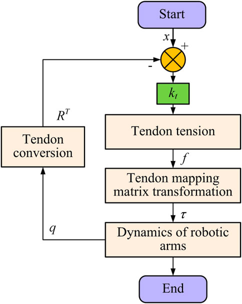
With Equations 1–6, the output flow of the tendon-driven actuator to the joint site can be obtained as denoted in Figure 2.

Figure 2

Figure 2. Output flow chart of the tendon-driven actuator.

Figure 2 shows the output process of the tendon-driven actuator to the joint site. Firstly, it sets the target tendon position vector $x$. Secondly, it calculates the difference between the target position vector and the actual tendon position vector to obtain the position error. Next, the linear spring modeling coefficient $k_t$ is used to adjust the position error, and the tendon tension vector $f$ is obtained. Then, the mapping matrix $R^{\prime }$ is used to convert $f$ into joint torque $\tau$. Finally, $\tau$ acts on the RA to generate joint angular displacement, and feedback the current $x$ value through $R^{\prime }$'s transpose matrix to complete the control loop.

2.2 Design of tracking control algorithm for tendon-driven robotic arm based on AARBF

In the field of RA control, with the increasing demand for intelligence and precise control, traditional control strategies have gradually become less flexible. In the last few years, various neural networks have been continuously applied in mechanical control, and RBF has been widely introduced into RA control systems because of its excellent nonlinear mapping ability and ability to approximate arbitrary continuous functions (Liu et al., 2023). In highly nonlinear systems such as tendon-driven RAs, the adaptive characteristics of RBF neural networks allow it to adjust control rules in real-time to adapt to external load changes and internal parameter disturbances, thereby achieving accurate trajectory tracking. The general structure of RBF is denoted in Figure 3.

Figure 3

Figure 3. RBF structure diagram.

The network structure of RBF is denoted in Figure 3. As a simple three-layer feedforward neural network, RBF mainly contains an input layer, a hidden layer, and an output layer. The input layer consists of source nodes, which directly receive external input data without performing any calculations. The hidden layer is the core of the RBF network, consisting of a series of neurons with radial basis activation functions. These activation functions typically use Gaussian functions, whose output depends on the Euclidean distance between the input vector and the center of the neuron. When the output of the hidden layer is transmitted to the output layer, the output layer weighted and summed these activation values to generate the final output of the network.

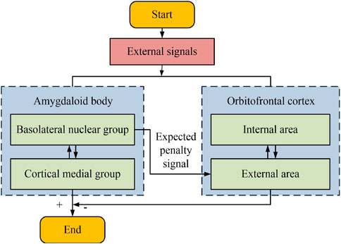
Traditional RBF networks have certain shortcomings in selecting center points and processing large amounts of noisy data, and have limited adaptability to dynamic environments. Therefore, the study introduced an emotion computing model to improve the effectiveness of RBF. The emotion computing model draws inspiration from the dynamic characteristics of human brain emotion processing, enabling the network to adaptively adjust parameters based on emotional changes, thereby improving the model’s adaptability and generalization ability (Mohammed Ali et al., 2022; Xian et al., 2023). In addition, the model is inspired by neurophysiology and a computational framework is established for emotional processing. Its general composition structure is shown in Figure 4.

Figure 4

Figure 4. Structural diagram of affective computing model.

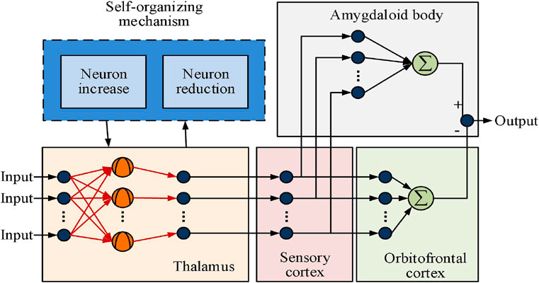
The basic structure of the affective computing model is denoted in Figure 4, which mainly includes two parts: the amygdala and the orbitofrontal cortex. The amygdala is composed of the basal lateral nucleus group and the cortical medial group, while the orbitofrontal cortex is composed of internal and external regions. The amygdala nucleus responds directly to internal emotional stimuli such as hunger or pain, while playing a crucial role in learning new associations between emotions and various stimuli. The orbitofrontal cortex is responsible for inhibiting established emotional responses, especially when these responses no longer adapt to changing environments or reward conditions. In summary, the affective computing model reveals the regulatory mechanisms of emotional learning and response, with the amygdala responsible for forming responses and the orbitofrontal cortex adjusting these responses when conditions change (Phuong and Cong, 2024). The AARBF, which combines affective computing, is denoted and its structure is denoted in Figure 5.

Figure 5

Figure 5. Structure diagram of AARBF combined with affective computation.

The structural diagram of AARBF is denoted in Figure 5. The complete AARBF is mainly composed of the thalamus, sensory cortex, orbitofrontal cortex, amygdala, and self-organizing mechanism. AARBF first receives various sensor data from the left side of the RA as input, such as displacement angle, velocity, or acceleration. Secondly, the input signal will first enter the thalamus and complete data analysis through RBF. The mathematical expression for this process is denoted in Equation (7).

$\begin{array}{cc}{\phi }_j=\exp \left(-\frac{{\displaystyle \sum _{i=1}^k}{\left(a_i-c_j\right)}^2}{{\left(b_j\right)}^2}\right)& j=1,2,\cdots ,n\end{array}(7)$

In Equation 7, $a_i=\left[a_1,a_2,\cdots ,a_i\right]$ represents the input signal. $c_j$ represents the center value of the activation function. $b_j$ represents the base width of the activation function. $n$ represents the amount of neural network nodes. Using the output value of the thalamus as input to the sensory cortex, the output of the sensory cortex will then enter the amygdala and orbitofrontal cortex, respectively. The output of the amygdala is denoted in Equation 8.

$E_1={\displaystyle \sum _{j=1}^n}{V}_j{\phi }_j=V^T\phi (8)$

In Equation 8, $E_1$ denotes the output of the amygdala. $\phi$ denotes threshold, $\phi =\left[{\phi }_1,{\phi }_2,\cdots ,{\phi }_j\right]$. $V$ represents the weight of the amygdala, $V=\left[V_1,V_2,\cdots ,V_j\right]$. V represents the transpose of $V$. The output of the orbitofrontal cortex is denoted in Equation 9.

$E_2={\displaystyle \sum _{j=1}^n}{W}_j^{\prime }{\phi }_j={W^{\prime }}^T\phi (9)$

In Equation 9, $E_2$ denotes the output of the orbitofrontal cortex. $W^{\prime }$ represents the weight of the orbitofrontal cortex, $W^{\prime }=\left[W_1^{\prime },W_2^{\prime },\cdots ,W_j^{\prime }\right]$. ${W^{\prime }}^T$ represents the transpose of $W^{\prime }$. According to Equations 8, 9, the final output value of AARBF can be obtained, as denoted in Equation 10.

$E_{total}=E_1-E_2={\left(V-W^{\prime }\right)}^T\phi (10)$

In Equation 10, $E_{total}$ represents the total output of AARBF.

An RA is a complex nonlinear system, whose complexity comes from strong coupling, multivariate characteristics, and environmental uncertainty. In practical applications, the positive definite inertia matrix, centripetal force, Coriolis force matrix, and gravity matrix all contain unknown dynamic parameters, which make it difficult for the dynamic model of the RA to achieve high-precision approximation. However, AARBF has self-learning ability and the ability to handle complex models, making it suitable for modeling and control of RA systems. To address the tracking and control challenges of tendon-driven RAs in unknown dynamic environments, the study proposes using AARBF for function approximation of dynamic models. The control process of AARBF in tendon-driven RAs is denoted in Figure 6.

Figure 6

Figure 6. Control flow chart of AARBF in tendon-driven manipulator.

In Figure 6, AARBF is used as the main control algorithm, while an improved PID controller is used in the controller block, which can handle complex dynamic behavior in nonlinear systems. In order to improve the adaptability and robustness of the system, the affective computing model is also introduced into the adaptive block, which combines RBF and affective processing mechanism, so that the control system can dynamically adjust the control parameters according to real-time affective feedback, so as to achieve more accurate trajectory tracking and control. Figure 6 shows the control process of AARBF in tendon-driven RAs. Firstly, the target joint position is used as a reference input and generate tendon tension through the controller. Secondly, tendon tension is used to calculate the actual joint torque of the RA, which is then used to the RA to drive the joint to its desired position. Next, the actual position of the RA is fed back to the control system and in contrast with the target position to calculate the position error. In addition, AARBF is used to receive position error information and adaptively adjust the control signal to reduce errors and improve tracking performance. The adaptive control mechanism combined with AARBF enables the RA control system to handle unknown or changing dynamic conditions, thereby achieving precise tracking control. Finally, the tendon tension output by the controller and the calculated joint torque can be dynamically adjusted to cope with the nonlinearity and uncertainty within the RA system.The weight diagram of the adaptive neural network for the tendon-driven robotic arm tracking control strategy is shown in Figure 7.

Figure 7

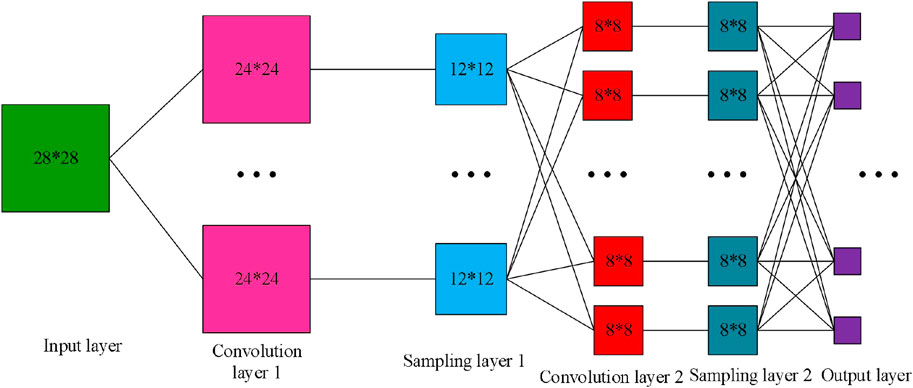
Figure 7. Weight plot of adaptive neural networks for tracking control strategies of the tendon-driven robotic arm.

In the Figure 7 is a weight plot of an adaptive neural network for tracking control strategies of the tendon-driven robotic arm. The neural network model consists of the input layer, two convolutional layers, two sampling layers (pooling layer) and the output layer. The input layer receives input data of 28 × 28 from sensors of the robotic arm, such as a joint angle, velocity, or acceleration. Convolution Layer 1 performs feature extraction on the input data, using the convolution kernel to slide on the input data to extract local features. These features may include edges, corners, etc., and are crucial for the motor state identification of the robotic arm. The first sampling layer (usually maximum pooling or average pooling) down samples the output of the convolution layer 1, reducing the spatial dimension of the data, thereby reducing the computational complexity and extracting more abstract features. The second convolutional layer further processes the output of the sampling layer 1 to extract higher-level features that may be related to the movement patterns of the robotic arm. The second sampling layer continues to downsample the feature data of the output mechanical part of the convolution layer 2, reducing the dimensionality of the feature data of the mechanical part while maintaining key features to inform the decision of the output layer. Finally, the output layer generates control signals that can be used to adjust the tendon tone of the robotic arm to achieve precise tracking control.

3 Results

To demonstrate the good tracking and control performance of AARBF, benchmark performance testing and simulation testing were set up in the study. In two tests, by comparing two other control methods, the performance of three control methods in fitness value, error accuracy, steady state, position tracking simulation, speed tracking simulation, control torque simulation, and system control error was studied, ultimately proving that AARBF has better control effect.

3.1 AARBF benchmark performance testing

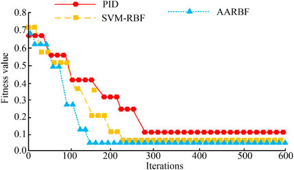
In this study, MATLAB R2022a software was used to model and simulate the tendine-driven RA, including Simulink toolbox and neural network toolbox. The simulation environment was configured as a computer equipped with Intel i7 processor and 16 GB memory, and a 3-DOF tendon-driven robot arm model was adopted. The control effects of PID, SVM-RBF and AARBF control algorithms were compared under the same initial conditions, and the evaluation indexes included error accuracy, steady state, convergence speed and maximum torque change. To demonstrate that AARBF has good control performance, its benchmark performance was first tested. PID and Support Vector Machine with Radial Basis Function (SVM-RBF) were selected as the two control algorithms for comparison. The simulation environment of the tendon-driven RA was set in MATLAB, and the fitness values of the three algorithms with the amount of iterations were obtained as denoted in Figure 8.

Figure 8

Figure 8. Iterative fitness values for different control algorithms.

Figure 8 shows the fitness values of three control algorithms at different iterations. As denoted in Figure 8, as the amount of iterations increased from 0 to 600, the fitness values of the three control algorithms indicated a continuous decreasing trend. Compared with PID and SVM-RBF, the AARBF algorithm designed in this study only required 138 iterations to reach steady state, and the fitness value of the AARBF algorithm was 0.05. PID and SVM-RBF required 275 and 226 iterations respectively to reach steady state, indicating that AARBF had faster convergence speed and better training performance. The error accuracy and steady-state of different control algorithms during the iteration process are shown in Figure 9.

Figure 9

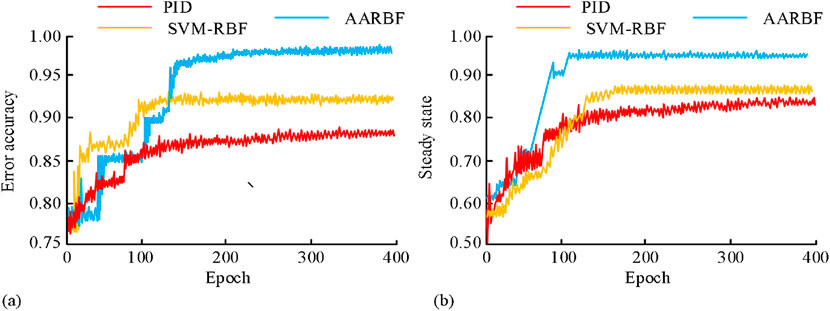
Figure 9. Error accuracy and steady state of different control algorithms. (A) Error variation under different control algorithms. (B) The variation of controlled variable q with different control algorithms.

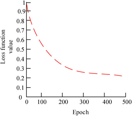
The error accuracy in Figure 9 refers to the error between the system output and the target trajectory, reflecting the system’s ability to track the target position. In Figure 9, the controlled variable q was used to measure the error accuracy. q represents the joint position of the RA, and its error accuracy is evaluated by the error between the system output and the target input qd. In addition, q is also the time response to the step input of the target position. By comparing the time response of the system output and the target input, the response performance and error accuracy of different control algorithms can be evaluated. Figures 9A, B show the error accuracy and stability of different control algorithms. In Figure 9A, when the parameters of Epoch increased from 0 to 400, the error accuracy of PID, SVM-RBF, and AARBF would also continue to increase. The highest error accuracy of PID, SVM-RBF, and AARBF was 0.86, 0.92, and 0.97, respectively. Figure 9B shows the steady state of different control algorithms under different iterations. Steady state is measured by how much the output fluctuates after the system reaches a stable state. The steady state of AARBF algorithm was 0.95 after reaching the stable state, which was better than PID and SVM-RBF algorithm. To demonstrate the convergence process of neural network weights, the loss function variation curve was used to illustrate, as shown in Figure 10.

Figure 10

Figure 10. Variation of model loss function.

In Figure 10, the AARBF loss function curve showed a significant decrease within 100 training iterations, a slow decrease between 100 and 200 training iterations, and convergence at around 300 training iterations. At this point, the loss function value was 0.24. The data showed that AARBF had a fast convergence speed, a small loss function value, and excellent performance.

3.2 Simulation results of tendon driven robotic arm control based on AARBF

After testing the benchmark performance of the three control algorithms, the simulation control of a 3-joint 4-tendon RA was studied using each of the three control algorithms. In the same environment, simulation tests were conducted to obtain the position tracking simulation outcomes of the RA joint 1 under three control algorithms, as shown in Figure 11.

Figure 11

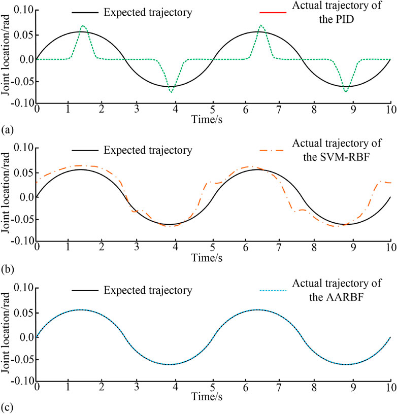
Figure 11. Simulation results of position tracking of the robotic arm under different control algorithms. (A) Simulation results of the position of joint 1 under PID control. (B) Simulation results of the position of joint 1 under SVM-RBF control. (C) Simulation results of the position of joint 1 under AARBF control.

Figures 11A–C respectively show the simulation outcomes of the position tracking of the RA joint 1 under different control algorithms. From Figure 11A, the actual position tracking curve under PID control almost did not coincide with the expected position tracking curve, indicating that the control effect of this control method differed significantly from the actual expected effect. From Figure 11B, the actual position tracking curve under SVM-RBF control partially overlapped with the expected position tracking curve, and the fluctuation range of the actual position tracking curve controlled by SVM-RBF was relatively small, indicating that the control effect of SVM-RBF was better than PID. According to Figure 11C, the expected position curve under AARBF control overlapped with the actual position curve, indicating that AARBF was able to complete the system’s control instructions and make the motion trajectory of the RA meet expectations. Next, joint 2 was tested to obtain the speed tracking simulation outcomes of the RA joint 2, as shown in Figure 12.

Figure 12

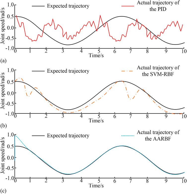
Figure 12. Simulation results of velocity tracking of the robotic arm under different control algorithms. (A) Simulation results of the speed of joint 2 under PID control. (B) Simulation results of the speed of joint 2 under SVM-RBF control. (C) Simulation results of the speed of joint 2 under AARBF control.

Figures 12A–C showcase the speed tracking simulation outcomes of the RA joint 2 under PID, SVM-RBF, and AARBF control, respectively. Based on Figure 12, the speed tracking simulation outcomes under PID control were the worst, with a significant difference between the actual and the expected values. The speed tracking simulation outcomes under AARBF control were the best, with the actual value basically overlapping with the expected value. The control effect of SVM-RBF was between the other two methods. Next, joint 3 was tested to obtain the simulation outcomes of the control torque of the RA joint 3, as shown in Figure 13.

Figure 13

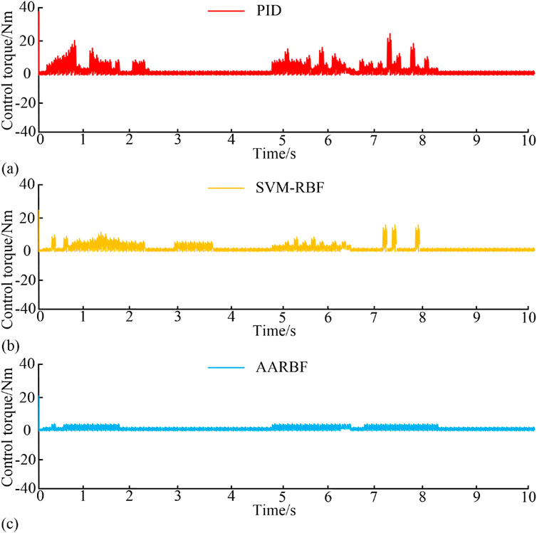
Figure 13. Torque of mechanical arm under different control algorithm simulation. (A) Simulation results of control torque of joint 3 under PID control. (B) Simulation results of control torque of joint 3 under SVM-RBF control. (C) Simulation results of control torque of joint 3 under AARBF control.

Figures 13A–C showcase the simulation outcomes of the control torque of the RA joint 3 under PID, SVM-RBF, and AARBF control, respectively. The max torque variation values under PID, SVM-RBF, and AARBF control could reach 24.1 Nm, 18.5 Nm, and 3.8 Nm, respectively. Compared with PID and SVM-RBF, the joint torque variation under AARBF control was smoother and the jitter was smaller, indicating that this control scheme had the best effect. Finally, test the system control error under three control schemes, as shown in Figure 14.

Figure 14

Figure 14. Time response results of different algorithm control errors.

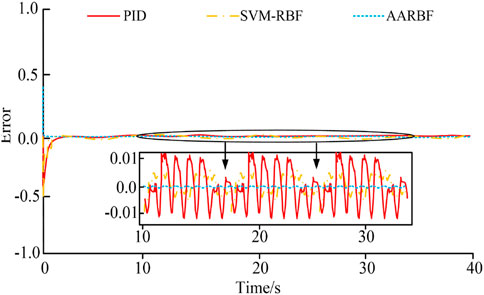
Figure 14 shows the overall control error values under PID, SVM-RBF, and AARBF control. As shown in Figure 14, the overall control error fluctuation ranges of PID, SVM-RBF, and AARBF were −0.012∼0.012, −0.005∼0.005, and −0.001∼0.001, respectively. The control strategy adopted in this study could achieve the minimum control error.

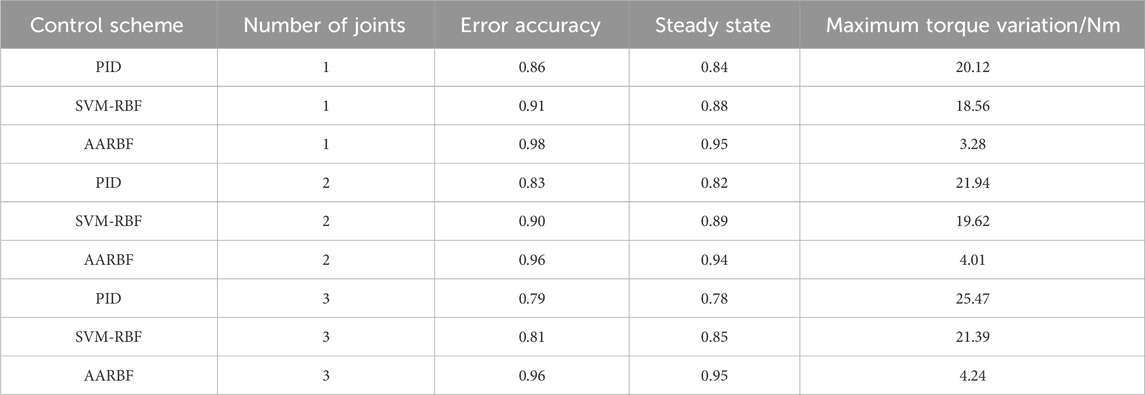
Table 1 shows the performance of PID, SVM-RBF and AARBF control schemes under different joint numbers. From Table 1, AARBF control scheme showed high error accuracy and stability under all joint numbers, with the highest error accuracy of 0.98 and the highest steady state of 0.95. At the same time, the maximum torque variation of the AARBF control scheme was also small, with a minimum of 3.28 Nm.

Table 1

Table 1. Send delay and transmission delay for different models in four networks.

4 Discussion

In this study, an AARBF network structure was designed by combining affective computing models with RBF, and this structure was used for precise tracking control of tendon-driven RAs. The research outcomes indicated that the AARBF algorithm performed well in multiple performance indicators, significantly better than traditional PID control algorithms and SVM-RBF algorithms. Specifically, the fitness value of AARBF algorithm in benchmark performance testing quickly reached 0.05, with 138 iterations, far lower than the iterations of PID and SVM-RBF, demonstrating its excellent convergence speed and high-precision control ability. In addition, the AARBF algorithm performed excellently in error accuracy. As shown in Figures 10, 11, the simulation outcomes of the joint position and velocity tracking of the RA under AARBF control perfectly coincided with the target curve, with almost no observable errors. However, the curves under PID and SVM-RBF control indicated significant deviations. This result highlighted the powerful ability of the AARBF algorithm in handling the nonlinear dynamics of tendon-driven RAs. In steady state testing, the AARBF algorithm also demonstrated its advantages. As shown in Figure 12, the tendon-driven RA using the AARBF algorithm maintained a relatively low torque change in the dynamic environment, with a maximum torque change of only 3.8 Nm, while the PID and SVM-RBF algorithms achieved torque changes of 24.1 Nm and 18.5 Nm, respectively. This indicated that AARBF could significantly reduce system jitter, thereby improving the overall stability and reliability of the system. Finally, the overall control error fluctuation range of the AARBF algorithm was extremely small, ranging from −0.001 to 0.001, which was much better than the control error fluctuation range of PID (−0.012 to 0.012) and SVM-RBF (−0.005 to 0.005), further verifying its superior performance in practical applications. In summary, the AARBF algorithm has significant advantages in tracking control of tendon driven RAs, especially in terms of error accuracy, stability, and adaptability to complex dynamic environments.

5 Conclusion

The research outcomes indicated that compared to PID and SVM-RBF, AARBF could not only converge to a stable state faster, but also significantly improved error accuracy and stability. Its amount of iterations to reach a stable state was 138, and the highest error accuracy and stability were 0.97 and 0.95, respectively. In the simulation experiment, the position tracking curve and speed tracking curve under AARBF control coincided with the expected curve, while the fluctuation amplitude of torque simulation was the smallest, and the maximum value of torque change was only 3.8 Nm. Ultimately, the overall control error within the range of −0.001∼0.001 could be achieved. In summary, AARBF has good performance in tendon driven RA control problems, but there are still some shortcomings in this study. Future work will focus on exploring the performance of composite control strategies in RA control problems, and exploring the potential of AARBF in different RA application scenarios by optimizing model parameters.

Data availability statement

The original contributions presented in the study are included in the article/supplementary material, further inquiries can be directed to the corresponding author.

Author contributions

DF: Conceptualization, Formal Analysis, Investigation, Methodology, Project administration, Supervision, Writing–original draft, Funding acquisition. FY: Data curation, Formal Analysis, Investigation, Resources, Software, Validation, Writing–review and editing.

Funding

The author(s) declare that financial support was received for the research, authorship, and/or publication of this article. The research is supported by: The Young and Middle-aged Talents Project funded by the Scientific Research Program of the Education Department of Hubei Province in 2022 (NO.Q20224506); Open Fund Project of Hubei Key Laboratory of Modern Manufacturing Quality Engineering in 2023(NO.KFJJ-2023009); 2022 Hubei Province High end Foreign Expert Project (No. 2022EJD027).

Conflict of interest

The authors declare that the research was conducted in the absence of any commercial or financial relationships that could be construed as a potential conflict of interest.

Publisher’s note

All claims expressed in this article are solely those of the authors and do not necessarily represent those of their affiliated organizations, or those of the publisher, the editors and the reviewers. Any product that may be evaluated in this article, or claim that may be made by its manufacturer, is not guaranteed or endorsed by the publisher.

References

Azizkhani, M., Godage, I. S., and Chen, Y. (2022). Dynamic control of soft robotic arm: a simulation study. IEEE Robotics Automation Lett. 7 (2), 3584–3591. doi:10.1109/lra.2022.3148437

CrossRef Full Text | Google Scholar

Fazilat, M., and Zioui, N. (2024). The impact of simplifications of the dynamic model on the motion of a six-jointed industrial articulated robotic arm movement. J. Robotics Control (JRC) 5 (1), 173–186. doi:10.18196/jrc.v5i1.20263

CrossRef Full Text | Google Scholar

Fazli, A., and Kazemi, M. H. (2024). Robotic arm tracking control through smooth switching LPV controller based on LPV modeling and torque approximation. Industrial Robot Int. J. Robotics Res. Appl. 51 (2), 246–257. doi:10.1108/ir-07-2023-0142

CrossRef Full Text | Google Scholar

Hsieh, Y. Z., Xu, F. X., and Lin, S. S. (2022). Deep convolutional generative adversarial network for inverse kinematics of self-assembly robotic arm based on the depth sensor. IEEE Sensors J. 23 (1), 758–765. doi:10.1109/jsen.2022.3222332

CrossRef Full Text | Google Scholar

Jeong, J. H., Shim, K. H., Kim, D. J., and Lee, S. W. (2020). Brain-controlled robotic arm system based on multi-directional CNN-BiLSTM network using EEG signals. IEEE Trans. Neural Syst. Rehabilitation Eng. 28 (5), 1226–1238. doi:10.1109/tnsre.2020.2981659

CrossRef Full Text | Google Scholar

Jiang, Y., Wang, Y., Miao, Z., Na, J., Zhao, Z., and Yang, C. (2020). Composite-learning-based adaptive neural control for dual-arm robots with relative motion. IEEE Trans. Neural Netw. Learn. Syst. 33 (3), 1010–1021. doi:10.1109/tnnls.2020.3037795

CrossRef Full Text | Google Scholar

Liu, Y. C., and Huang, C. Y. (2021). DDPG-based adaptive robust tracking control for aerial manipulators with decoupling approach. IEEE Trans. Cybern. 52 (8), 8258–8271. doi:10.1109/tcyb.2021.3049555

CrossRef Full Text | Google Scholar

Liu, Z., Peng, K., Han, L., and Guan, S. (2023). Modeling and control of robotic manipulators based on artificial neural networks: a review. Trans. Mech. Eng. 47 (4), 1307–1347. doi:10.1007/s40997-023-00596-3

CrossRef Full Text | Google Scholar

Mishani, I., and Sintov, A. (2021). Real-time non-visual shape estimation and robotic dual-arm manipulation control of an elastic wire. IEEE Robotics Automation Lett. 7 (1), 422–429. doi:10.1109/lra.2021.3128707

CrossRef Full Text | Google Scholar

Mohammed Ali, H., Hashim, Y., and A, A. L.-S. G. (2022). Design and implementation of Arduino based robotic arm. Int. J. Electr. Comput. Eng. 12 (2), 1411. doi:10.11591/ijece.v12i2.pp1411-1418

CrossRef Full Text | Google Scholar

Phuong, L. H., and Cong, V. D. (2024). Control the robot arm through vision-based human hand tracking. FME Trans. 52 (1), 37–44. doi:10.5937/fme2401037p

CrossRef Full Text | Google Scholar

Piqué, F., Kalidindi, H. T., Fruzzetti, L., Laschi, C., Menciassi, A., and Falotico, E. (2022). Controlling soft robotic arms using continual learning. IEEE Robotics Automation Lett. 7 (2), 5469–5476. doi:10.1109/lra.2022.3157369

CrossRef Full Text | Google Scholar

Purohit, J., and Dave, R. (2023). Leveraging deep learning techniques to obtain efficacious segmentation results. Archives Adv. Eng. Sci. 1 (1), 11–26. doi:10.47852/bonviewaaes32021220

CrossRef Full Text | Google Scholar

Shafei, A. M., and Mirzaeinejad, H. (2021). A novel recursive formulation for dynamic modeling and trajectory tracking control of multi-rigid-link robotic manipulators mounted on a mobile platform. Proc. Institution Mech. Eng. Part I J. Syst. Control Eng. 235 (7), 1204–1217. doi:10.1177/0959651820973900

CrossRef Full Text | Google Scholar

Shen, D., and Saab, S. S. (2021). Noisy-output-based direct learning tracking control with Markov nonuniform trial lengths using adaptive gains. IEEE Trans. Automatic Control 67 (8), 4123–4130. doi:10.1109/tac.2021.3106860

CrossRef Full Text | Google Scholar

Tan, N., Yu, P., Zhong, Z., and Ni, F. (2022). A new noise-tolerant dual-neural-network scheme for robust kinematic control of robotic arms with unknown models. IEEE/CAA J. Automatica Sinica 9 (10), 1778–1791. doi:10.1109/jas.2022.105869

CrossRef Full Text | Google Scholar

Tanaka, K., Minami, Y., Tokudome, Y., Inoue, K., Kuniyoshi, Y., and Nakajima, K. (2022). Continuum-body-pose estimation from partial sensor information using recurrent neural networks. IEEE Robotics Automation Lett. 7 (4), 11244–11251. doi:10.1109/lra.2022.3199034

CrossRef Full Text | Google Scholar

Xian, Y., Huang, K., Zhen, S., Wang, M., and Xiong, Y. (2023). Task-driven-based robust control design and fuzzy optimization for coordinated robotic arm systems. Int. J. Fuzzy Syst. 25 (4), 1579–1596. doi:10.1007/s40815-023-01460-x

CrossRef Full Text | Google Scholar

Xu, K., and Wang, Z. (2023). The design of a neural network-based adaptive control method for robotic arm trajectory tracking. Neural Comput. Appl. 35 (12), 8785–8795. doi:10.1007/s00521-022-07646-y

CrossRef Full Text | Google Scholar

Zahaf, A., Bououden, S., Chadli, M., and Chemachema, M. (2022). Robust fault tolerant optimal predictive control of hybrid actuators with time-varying delay for industrial robot arm. Asian J. Control 24 (1), 1–15. doi:10.1002/asjc.2444

CrossRef Full Text | Google Scholar