Force-controlled pose optimization and trajectory planning for chained Stewart platforms

Introduction: We study optimization methods for poses and movements of chained Stewart platforms (SPs) that we call an “Assembler” Robot. These chained SPs are parallel mechanisms that are stronger, stiffer, and more precise, on average, than their serial counterparts at the cost of a smaller range of motion. By linking these units in a series, their individual limitations are overcome while maintaining truss-like rigidity. This opens up potential uses in various applications, especially in complex space missions in conjunction with other robots.

Methods: To enhance the efficiency and longevity of the Assembler Robot, we developed algorithms and optimization models. The main goal of these methodologies is to efficiently decide on favorable positions and movements that reduce force loads on the robot, consequently minimizing wear.

Results: The optimized maneuvers of the interior plates of the Assembler result in more evenly distributed load forces through the legs of each constituent SP. This optimization allows for a larger workspace and a greater overall payload capacity. Our computations primarily focus on assemblers with four chained SPs.

Discussion: Although our study primarily revolves around assemblers with four chained SPs, our methods are versatile and can be applied to an arbitrary number of SPs. Furthermore, these methodologies can be extended to general over-actuated truss-like robot architectures. The Assembler, designed to function collaboratively with several other robots, holds promise for a variety of space missions.

1 Introduction

Robotic space missions are complex, expensive endeavors, often resulting in multiple mission extensions or scope expansions to maximize the robotic system’s potential over its useful lifespan. Ensuring that a system is precise and robust enough to accomplish its mission in addition to unknown future mission requirements drives up development and deployment costs significantly, especially due to one-off hardware design. The overall cost of system deployment can be driven down by the mass production of smaller, modular robots that can join together to enhance their capabilities. Specifically, we seek to use parallel mechanisms called SPs, which are typically stiffer, more precise, and more robust to vibration than their serial counterparts of similar quality, at the cost of a smaller range of motion (Majid et al., 2000). Linking these units in a series overcomes their individual limitations and yet maintains their trusslike rigidity, enabling their potential use for various purposes. We designate such a configuration as an “Assembler” robot. The origin of this idea came from previous research at NASA Langley Research Center which has also continued development in parallel with different physical Assembler hardware (Cooper et al., 2022; Moser and Cooper, 2019). While the number of SPs in a stack is arbitrary, the experimentation discussed in this article concerns stacks of four. A stack of SPs has the property that it is over-actuated, which implies that there is a continuum of internal plate poses for any pair of end plate poses. This allows internal plate poses be chosen to satisfy constraints and optimize a variety of metrics. The objective of this research is to maneuver the interior plates of the Assembler such that the load forces distributed through the legs of each constituent SP are balanced, allowing for a larger workspace and a greater overall payload capacity.

We propose to use these chained SPs as an alternative to robot serial arms, for eventual use in fully automated robot assembly on the Moon or in space. Each SP consists of a pair of plates with six legs in between. The structure is actuated simply by extending or contracting the linear actuator legs. An example of the structure is shown in Figure 1.

FIGURE 1

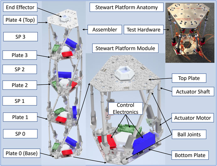
FIGURE 1. Anatomy of an Assembler Robot. The robot is comprised of four chained six degrees of freedom (DOF) SPs, giving it a larger range of motion and total 24 DOF. Each SP is comprised of six linear actuators mounted between two plates, since the stacked SPs share plates the Assembler has a total of 5 plates that serve as the upper and lower boundaries of each SP. The legs are connected via ball joints that are mounted below and above each plate. Thus, the leg connections do not lie in the same plane as the plates.

Stacks of SPs, like the Assembler, combine the strength and stability of truss-like SPs, with the reach that serially linked robots such as Universal Robotics UR-10 can provide without the mass inherent to large actuators responsible for driving serial mechanisms. The construction of an SP of the type presented in this paper - six linear actuators separating two parallel plates presents precision and extreme stiffness (Li et al., 2002) as linear actuators cannot be easily backdriven (and hold their positions with no power applied). Position holding lends itself to the optional application of the SP-Stack as semi-permanent long-term reconfigurable support truss structures. The high stiffness also means higher fundamental frequency and lower oscillation amplitude (i.e., cantilevering is less of an issue). The stacking of the individual platforms to make a larger robot extends the reach by multiplying the workspace configurations, yielding a 24 total DOF robot (or more, if necessary). This overactuation opens up optimization, as near-infinite internal configurations can yield the same end effector pose. In addition, the extreme overactuation present in the system allows for redundancy. If any individual actuator fails, the robot is capable of compensating for the failure, increasing the robustness of the system. The methods shown in this paper are applicable to a range of similarly configured truss-like robots, not limited to this particular 24DOF configuration. SP mechanisms are not perfect however, having poor passive compliance, limited velocity, and limited angular range of motion. The poor passive compliance can be compensated for with active compliance, but restricted angular range of motion is a limiting factor that must be considered in choosing applications for this system, though it can be partially compensated for with a spherical wrist at the end effector, or an off-axis turntable system at the base.

We propose an optimization approach to reduce structural forces in poses and throughout motion. The complexity of the problem stems from the serial combination of parallel kinematic structures (each SP), which can render difficult the problem of even finding feasible poses for a given end effector position and load. From an optimization perspective, the primary source of complexity stems from nonlinearity and nonconvexity of the feasible space, resulting from the trigonometric functions required to model the physical kinematic transformations throughout the structure, along with the many other bilinear and quadratic terms. These include coordinate distance computations to determine leg lengths, wrench and force computations, and coordinate transformations after the computation of the transformation matrices.

There have been many works in the literature exploring design optimization of individual SPs, including (Chen et al., 2007; Bangjun et al., 2012; Lei and Xiaolin, 2013; Toz and Kucuk, 2013; Xie et al., 2017; Sun and Lian, 2018; Ríos et al., 2021). These works typically optimize the design of a single SP with respect to parameters such as stiffness, manipulability, and accuracy. In particular, (Zhang, 2005), designs and implements a variant of SP with passive control of leg forces. However, we found the literature on stacked SPs to be incredibly sparse, and were unable to find any prior works optimizing poses for stacked SP chains based on leg forces. There is a related field studying more general actuated truss structures, such as in (Miura and Furuya, 1988; Dorsey et al., 1992; Yokoi et al., 1992; Williams, 1995). Among other structures, these works study variable geometry truss (VGT) structures, which are similar to SP’s, except that each plate is replaced with a triangle of three actuated legs, and the legs between ‘plates’ are not actuated. (Yokoi et al., 1992; Williams, 1995) also studied a version of an SP where the plates are replaced with triangles of stiff legs. However, none of these works study the problem of controlling forces while maneuvering these devices.

For trajectory planning, state-of-the-art approaches include the random tree search-based method RRT (LaValle, 1998) and variants RRT-Connect (Kuffner and LaValle, 2000), RRT* (Karaman and Frazzoli, 2011), RRT*-SMART (Islam et al., 2012), among others. Other state-of-the-art approaches include CHOMP (Zucker et al., 2013), TrajOpt (Schulman et al., 2014), and ROMP (Quintero-Pena et al., 2021). A number of works have explored trajectory planning for individual SP’s, including (Nguyen and Antrazi, 1990; Nguyen et al., 1991; Cortes and Simeon, 2003; Grosch et al., 2010; Wang et al., 2015; Ernandis, 2021). Several such works, such as (Cortes and Simeon, 2003; Ernandis, 2021), rely on variants of RRT. In one example (Cooper et al., 2022; Cortes and Simeon, 2003), even applies this method to an obstacle-avoiding trajectory planning problem for a 4-stack of SPs. (Balaban et al., 2019). performs stiffness optimization on a 2-D version of the stacked platform structure. Aside from RRT variants, some obstacle-avoiding trajectory planning approaches applied primarily to simple structures such as serial arms are introduced in (Zucker et al., 2013; Schulman et al., 2014; Osa et al., 2017). Prior works involving trust-region based approaches for trajectory planning, as used in this work, include (Dragan and Srinivasa, 2014; Ichnowski et al., 2020; Quintero-Pena et al., 2021) for serial arms, and (Szynkiewicz and Błaszczyk, 2011; Santos and da Silva, 2017; Volz and Graichen, 2018) for more difficult robots involving closed kinematic chains.

We were unable to find any works in the literature performing any sort of force-controlled trajectory planning of stacked SPs in three dimensions, with very few performing any sort of trajectory planning for stacked SPs. Such optimization can significantly improve maximum leg forces throughout the structure, thereby increasing the workspace of an SP under large loads.

1.1 Contributions

1.1.1 Pose Optimization

We present an optimization approach to solve the inverse kinematic pose optimization problem. We model the problem as a quadratically constrained quadratic program (QCQP). We are not aware of prior models for chained Stewart platforms, though for a single SP, (Bingul and Karah, 2012), gives a dynamic model. We propose two heuristics to generate initial poses with a given target end effector position and load: (1) a spline-based heuristic and (2) a simple closed-form initialization approach for which each SP has the same pose. Note that these heuristics might fail to generate a feasible pose. This is one of the inherent difficulties in the problem of even detecting if there is a kinematically valid pose given a certain end effector. We then optimize the QCQP by feeding the model a feasible initial solution to the local optimal solver IPOPT. The optimization process typically takes just over 1 s on average for a single pose, for an Assembler consisting of four chained SPs. We computationally demonstrate the effectiveness of the approach, and demonstrate the effectiveness of the method in improving the force-valid range of motion of the assembler compared to the spline-based heuristic See (Figure 2A).

FIGURE 2

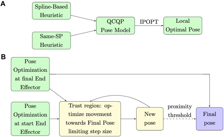
FIGURE 2. (A) Pose Optimization Flowchart (B) Trajectory Optimization Flowchart.

1.1.2 Trajectory Optimization

We extend the pose optimization model to compute trajectories that reduce the overall force on the machine when moving between end effectors. We enable this possibility through a trust region subproblem and show that generates quality movements efficiently. We demonstrate that our approach significantly improves upon a naive transformation.

In other tests, our approach significantly outperforms an RRT* implementation. We do not include the RRT* in this paper as it was suboptimal to our trust region method See (Figure 2B).

1.1.3 Outline

In Section 2 we describe the structure of the Assembler and its abilities in terms of movement and positions. We then introduce the forward and inverse kinematics problems for single SP’s and the full Assembler, and mathematically define a kinematically valid SP. In Section 3.3, we propose a spline-based construction heuristic (SIK) to produce valid poses. We also propose a simpler same-SP heuristic to produce starting solutions for the optimizer. In Section 3.4, we propose an optimization model and simple initial-solution scheme (OPT) to directly generate locally force-optimal poses. In Section 4.2, we propose a trust region approach for trajectory planning based on the optimization model. In Section 5.2, we compare the effectiveness of the SIK and OPT schemes to quickly generate workable poses for the Assembler. In Section 5.3, we compare the trust region trajectory planning scheme with a naive approach based on linearly interpolating leg lengths between the initial and target poses. Finally, in Section 5.4, we demonstrate the effectiveness of the optimizer in improving the achievable range of motion of the Assembler.

2 Assembler robot, notation, and transformations

A Stewart platform consists of a pair of plates linked by six linear actuators, constituting a parallel mechanism with six degrees of freedom (DOF). The actuators for each platform are connected via ball joints on either end. We refer to the linear actuators as legs. The motor of each actuator is situated on the leg bottom (LB), while the shaft of the actuator is on the leg top (LT). We define the pose of a plate as its position and orientation in a given reference frame, and we characterize the pose of an Assembler via the poses of its plates in the Assembler’s reference frame, also referred to as the global reference frame. That is, a pose is a list of plate positions ${\mathbf{p}}_i^{\mathcal{G},P}$ and rotations ${\mathbf{r}}_i^{\mathcal{G},P}$ for each plate i with i = 0, …, N_P. See Figure 3B. The pose of each SP can be expressed in terms of the pose of its top plate in the reference frame of its bottom plate. We primarily use this local ‘SP-frame’ to mathematically define a kinematically valid SP. See Figure 3C for examples of local reference frame variables.

FIGURE 3

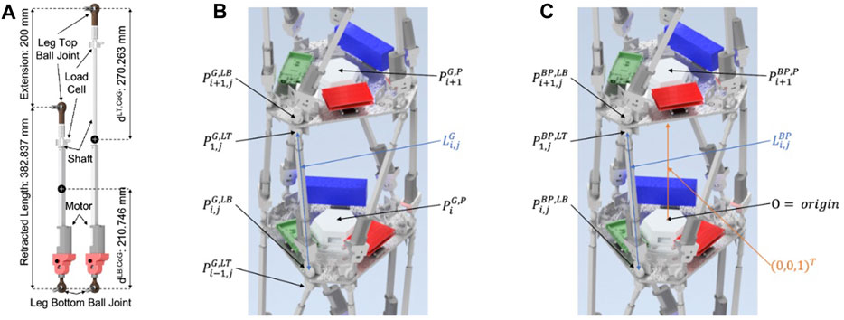
FIGURE 3. (A) Image of a linear actuator in two positions. The legs of the assembler are made from these linear actuators. Linear actuator has two parts: the motor (on the leg bottom) and the shaft (on the leg top). The actuator works by extending and contracting the shaft. For force computations, we record as data the distance from the bottom of the leg to the center of gravity of the motor, and from the top of the leg to the center of gravity of the shaft. (B) A section of the Assembler with several variable locations labeled in the global reference frame. Note that the center of gravity of plate i is ${\mathbf{p}}_i^{\mathcal{G},P}$. Variables in the global reference frame are denoted that a superscript $\mathcal{G}$. (C) The same pose, but rotated to look from the reference frame $\mathcal{B}\mathcal{P}$ of SP i with respect to the bottom plate. We also occasionally use $\mathcal{T}\mathcal{P}$ to denote the reference frame with respect to the top plate of the SP.

Note that, crucially, a top plate pose is not uniquely defined by only the leg lengths (Lazard and Merlet, 1994; Charters et al., 2009).

An important pose is the resting pose. We define this as the pose where all the legs are set to be 50% of their total possible length, as a heuristic estimate of the center of a SP’s workspace. We define parameters L^rest for each leg as the vector that leg follows when in resting pose. Note that, in the resting pose, due to the symmetry of the SP design used here, each plate is translated vertically with no rotation, so that ${\mathbf{r}}_i=\mathbb{0}$ and ${\mathbf{p}}_{i,[1:2]}=\mathbb{0}$.

We use $\mathbb{0}$ to denote a vector or matrix of zeros, and we leave size of this vector/matrix to be deduced by context.

Given a goal position for the end effector of the Assembler, the goal of this work is to quickly find kinematically valid poses and motions for a given Assembler while controlling the worst-case forces on the legs. We consider only mass-related forces and external forces applied to the end-effector of the Assembler, and neglect any external forces applied to other parts of the Assembler by e.g., wind.

To resolve torques resulting from the masses of each leg, we must compute the center of gravity (CoG) for each part the leg. Crucially, the CoG for a leg is not in the center of each leg; rather, each leg is a linear actuator consisting of two connected parts, a motor and a shaft. See Figure 3A. The CoG of each part is a fixed distance from its attachment location. This fixed-distance property gives the model for the CoG a measure of mathematical complexity, as one cannot simply multiply the vector defining the leg’s position by a fixed number to obtain the position of the center of gravity for each part. Rather, the unit vector defining the direction of the leg is multiplied by the fixed distance from the attachment location of a part to its CoG. In this work, the motor of each leg is connected to the bottom plate of its SP, while the shaft is connected to the top plate.

In the remainder of this section, we first define our notation and mathematics for coordinate transformations. We then define the forward kinematics and inverse kinematics problems for an Assembler and for a single SP, define a kinematically valid SP, and give some reasoning for the use of four SPs for the Assembler in this work.

2.1 Notation

In this section, we introduce some useful notation and abbreviations to be used in the remainder of this work.

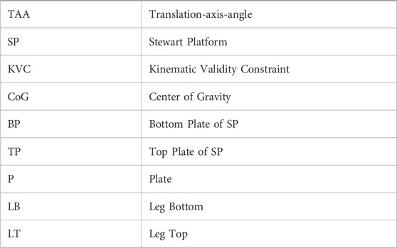
Shorthand: Here, we summarize our shorthand notation. TAA, SP, and KVC are used in text descriptions, while the rest are used in variable superscripts as object specifiers.

For parameter and variable definitions, we use the following notation,

$VarTyp{e}_{\mathit{V\; arIndex,[V\; alIndex]}}^{\text{RefFrame}\left(\text{Optional}\right),\text{DesiredObject},\text{specifier}(Optional)},(1)$

where RefFrame is the reference frame, VarIndex gives indices for the related object, and ValIndex gives vector and matrix indices. We implicitly define the reference frame of a plate by its leg attachment locations. The reference frame for each plate of an SP has its origin at the center of its exterior surface, the surface opposite its leg joints. In the Assembler stack, the top plate of each SP joins the bottom plate of the next at the plate centers, so that so that the two plates share the same origin, with the top SP rotated by 30°. To simplify calculations, we treat the top bottom plate of a SP and the top plate of the preceding SP as a single plate, providing only a single reference frame. This is accomplished by rotating the leg attachment locations for the bottom SP by 30° about the z-axis to obtain the leg attachment locations for the top SP.

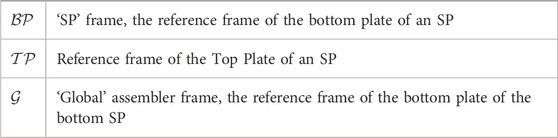
Reference Frames: These three reference frames are used throughout the 536 paper.

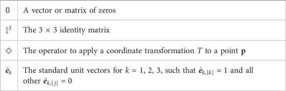
Miscellaneous Notation: We aggregate some useful miscellaneous notation here for reference.

2.2 Coordinate transformations

We use ‖ ⋅‖ to denote the 2-norm (Euclidean norm). For a vector v, we use $\widehat{\mathit{v}}$ to denote v/‖v‖, that is, the unit direction of v. We define ${\widehat{\mathit{e}}}_k\in {\mathbb{R}}^3$ for k = 1, 2, 3 as the standard unit vectors with indices starting at 1. That is, ${\widehat{\mathit{e}}}_1={[\mathrm{1,0,0}]}^{\top }$, ${\widehat{\mathit{e}}}_2={[\mathrm{0,1,0}]}^{\top }$, and ${\widehat{\mathit{e}}}_3={[\mathrm{0,0,1}]}^{\top }$.

We use ϒ to denote coordinate transformations via a vector containing the Translation-Axis-Angle representation (TAA)

$\mathbf{\Upsilon }=\left(\begin{array}{c}\hfill \mathbf{p}\hfill \\ \hfill \mathbf{r}\hfill \end{array}\right)=\left(\begin{array}{c}\hfill \mathbf{p}\hfill \\ \hfill \Vert \mathbf{r}\Vert \widehat{\mathbf{r}}\hfill \end{array}\right)=\left(\begin{array}{c}\hfill \mathbf{p}\hfill \\ \hfill \theta \widehat{\mathbf{r}}\hfill \end{array}\right).(2)$

The TAA format is used to represent position p and orientation data r in place of transformation matrices because total translational and rotational errors can be found by taking the norm of the top 3 and the bottom 3 components, respectively.

The related rotation matrix can be defined via Rodrigues’ formula as

$\mathbf{R}:=e^{\left[\mathbf{r}\right]}=I+\sin \left(\Vert \mathbf{r}\Vert \right)\frac{\left[\mathbf{r}\right]}{\Vert \mathbf{r}\Vert }+\left(1-\cos \left(\Vert \mathbf{r}\Vert \right)\right)\frac{{\left(\left[\mathbf{r}\right]\right)}^2}{\Vert \mathbf{r}{\Vert }^2},(3)$

where [r] is the vector cross-product operator for r

$\left[\mathbf{r}\right]≔\left[\begin{array}{ccc}\hfill 0\hfill & \hfill -r_3\hfill & \hfill r_2\hfill \\ \hfill r_3\hfill & \hfill 0\hfill & \hfill -r_1\hfill \\ \hfill -r_2\hfill & \hfill r_1\hfill & \hfill 0\hfill \end{array}\right]$

so that, for any vector v, we have [r]v = r ×v. We use the TAA scheme to represent reference frames in space due to its compactness, with the theoretically minimal six degrees of freedom, combined with the mathematical ease of converting the translational and rotational components to matrix transformation form. The matrix R is used to define transformation matrices via

$\mathbf{T}=\left[\begin{array}{cc}\hfill \mathbf{R}\hfill & \hfill \mathbf{p}\hfill \\ \hfill \mathbb{0}\hfill & \hfill 1\hfill \end{array}\right].(4)$

To apply the coordinate transformation defined by transformation matrix T to a point $\tilde{\mathbf{p}}$, we use

$\mathbf{T}\diamond \tilde{\mathbf{p}}≔{\left(\mathbf{T}\left(\begin{array}{c}\hfill \tilde{\mathbf{p}}\hfill \\ \hfill 1\hfill \end{array}\right)\right)}_{\left[1:3\right]}=\mathbf{R}\tilde{\mathbf{p}}+\mathbf{p}.(5)$

Where, for a vector v, we use a bracketed MATLAB style subscript to denote components; for example, we define ${\mathit{v}}_{[1:3]}={[v_1,v_2,v_3]}^{\top }$.

2.3 Forward and inverse kinematics

There are two primary problems of interest to solve for a general robot with an end-effector: the forward kinematics (FK) and inverse kinematics (IK) problems. The FK problem is to compute the end-effector pose given the actuator lengths. Conversely, the IK problem is to compute the actuator values given the end-effector pose.

For a single SP, the FK problem corresponds to computing the pose of the top plate w.r.t. the bottom plate given a vector of leg lengths. However, in general, the FK problem is difficult: it has multiple reachable solutions (Lazard and Merlet, 1994; Charters et al., 2009), most of which cannot be reversed, such as “pretzeled” poses for which the SP has twisted excessively, and spirals downwards until the legs collide. On the other hand, the IK problem corresponds to computing the leg lengths of the SP given the pose of the top plate w.r.t. the bottom plate. This computation is straightforward, with a simple closed-form solution, as described below. In this section, we describe all computations in the reference frame of the SP.

Define the pose of the top plate of an SP as T^TP, and let J be the set of legs for the SP. Then, for each leg of an SP, there are corresponding rest positions for the leg’s joint attachment locations to the top and bottom plates. For a leg j ∈ J, these are ${\mathbf{p}}_j^{\mathcal{T}\mathcal{P},\text{LT},\text{rest}}$ for the top plate and ${\mathbf{p}}_j^{\text{LB}}$ for the bottom plate. These locations are defined in the reference frame of the corresponding plate, and are required for leg-vector and leg-length computations. We compute the coordinates of the top-plate leg joint locations via

$\begin{array}{ccc}\hfill {\mathbf{p}}_j^{\text{LT}}& ={\mathbf{T}}^{\text{TP}}\diamond {\mathbf{p}}_j^{\mathcal{T}\mathcal{P},\text{LT},\text{rest}}\hfill & j\in J.\hfill \end{array}(6)$

Note that the bottom-plate joint attachment locations p^LB are known constants. Once joint locations have been determined, it is straightforward to calculate the resulting leg lengths by taking the magnitude of the positional displacement between corresponding leg joint pairs, as

${\mathit{L}}_j^{\mathrm{l}\mathrm{e}\mathrm{n}}=\Vert {\mathbf{p}}_j^{\text{LT}}-{\mathbf{p}}_j^{\text{LB}}\Vert j\in J.(7)$

The vector of leg lengths ${\left({\mathit{L}}_j^{\mathrm{l}\mathrm{e}\mathrm{n}}\right)}_{j\in J}$ is then the solution to the single-SP IK problem.

Considering that IK on an SP is a single step mathematical computation (Lynch and Park, 2017), it lends itself to rapid successive iteration. Solutions to the FK problem for SPs are based in this principle, with most algorithms performing calls to IK in order to numerically approximate the true position. However, as FK is not an integral component to the Assembler IK methodologies described in this paper, it is not described here in full. For further information, consult (Merlet, 2006).

For an Assembler consisting of a serial chain of stacked SP’s, which are parallel kinematic structures, neither the FK or IK problems are straightforward to solve. For the IK problem, there is generally a continuous space (or set of disjoint continuous spaces) of feasible plate positions for a given end-effector position. Moreover, this space is difficult to characterize, and can contain many bad solutions, such as those with extreme SP poses or very high leg forces. As such, before computing the leg lengths, one must first choose a ‘good’ solution for the plate positions from the space of feasible solutions. On the other hand, to solve the FK problem for an Assembler, one must individually solve the difficult FK problem for each SP.

In this work, we focus on solving the IK problem for an Assembler. We then extend our approach via a trust region method to solve point-to-point trajectory planning.

2.4 Kinematic validity constraints

In this section, we define what it means for an SP to have a valid pose. In this section, we will define constraints in the reference frame of the base plate of SP, so that the origin is the center of the bottom of the bottom plate of the SP, with no rotation. In effect, we omit the reference frame superscript $\mathcal{B}\mathcal{P}$, as defined in the following section.

Leg Length Bounds: The legs have minimum and maximum lengths that can be attained. For the robots we consider here, the legs all have uniform length bounds L^min and L^max, but this is easily changed in our model if more general situations are of interest. Formally, for a particular leg, let ${\mathbf{p}}^{\mathrm{LT}}$ and p^LB be the coordinates of the top and bottom connections of the leg. Then the vector $\mathit{L}={\mathbf{p}}^{\mathrm{LT}}-{\mathbf{p}}^{\mathrm{LB}}$ describes the direction and magnitude of the leg. This vector is then bounded in magnitude as

$L^{\min }\le \Vert \mathit{L}\Vert \le L^{\max }.(8)$

Note that, in the reference frame of the SP, the bottom-plate attachment locations p^LB are known constants.

Leg Angular Deviation: Each leg must not exceed a certain angular deviation from its normal resting pose, as this could break the ball joints in physical hardware. We must constrain the leg lengths in both the top and bottom pose.

Formally, for a particular leg, let p^LT,rest and p^LB,rest be the rest coordinates of the top and bottom connections of the leg. Then the vector L^rest = p^LT,rest − p^LB,rest describes the direction and magnitude of the leg in the resting pose.

The bottom-plate constraint for leg angle deviation is

$\begin{array}{c}\hfill \cos \left({\theta }^{\max }\right)\le \frac{\mathit{L}}{\Vert \mathit{L}\Vert }\cdot \frac{{\mathit{L}}^{\text{rest}}}{\Vert {\mathit{L}}^{\text{rest}}\Vert }.\end{array}(9)$

Similarly, we require the same constraints for the top plate angles. Let R be the rotation matrix defining the orientation of the top plate w.r.t. the bottom plate. Then the top-plate angles are defined as in (9), except that the rest coordinates are pre-multiplied by R to move them to the top plate, yielding

$\begin{array}{c}\hfill \cos \left({\theta }^{\max }\right)\le \frac{\mathit{L}}{\Vert \mathit{L}\Vert }\cdot \frac{\mathbf{R}{\mathit{L}}^{\text{rest}}}{\Vert \mathbf{R}{\mathit{L}}^{\text{rest}}\Vert }.\end{array}$

Since rotation operations are distance-invariant, we have $\Vert \mathbf{R}{\mathit{L}}^{\text{rest}}\Vert =\Vert {\mathit{L}}^{\text{rest}}\Vert$, yielding

$\begin{array}{c}\hfill \cos \left({\theta }^{\max }\right)\le \frac{\mathit{L}}{\Vert \mathit{L}\Vert }\cdot \frac{\mathbf{R}{\mathit{L}}^{\text{rest}}}{\Vert {\mathit{L}}^{\text{rest}}\Vert }.\end{array}(10)$

Legs Point Up: To prevent legs from colliding with the base plate of an SP, we require that each leg is pointing ‘up’, so that the z-component ${\mathit{L}}_{\left[3\right]}$ of $\mathit{L}$ is nonnegative:

${\mathit{L}}_{\left[3\right]}\ge 0.(11)$

Extreme Pose Prevention: We wish to prevent extreme and difficult-to-reach poses for each SP, particularly “pretzeling,” a phenomenon where the top plate of an SP over-rotates in the z-direction, causing it to collapse, spinning down until the legs of the SP collide. See e.g., (Zhang, 2005; Charters et al., 2009) for more information on singularities, such as pretzeling, that can be encountered with some SP designs. To help prevent such extreme poses, we set a limit of θ^R, max for the action of the plate rotation matrix R on any principle unit vector ${\widehat{\mathit{e}}}_k$, where k ∈ {1, 2, 3}. This corresponds to enforcing that each deviation angle ${\theta }_k^{\mathbf{R}}\le {\theta }^{\mathbf{R},\max }$, which is equivalent to

$\Vert {\widehat{\mathit{e}}}_k\Vert \Vert \mathbf{R}{\widehat{\mathit{e}}}_k\Vert \cos \left({\theta }_k^{\mathbf{R}}\right)={\widehat{\mathit{e}}}_k^{\top }\mathbf{R}{\widehat{\mathit{e}}}_k\ge \Vert {\widehat{\mathit{e}}}_k\Vert \Vert \mathbf{R}{\widehat{\mathit{e}}}_k\Vert \cos \left({\theta }^{\mathbf{R},\max }\right).$

Now, since $\Vert {\widehat{\mathit{e}}}_k\Vert =\Vert \mathbf{R}{\widehat{\mathit{e}}}_k\Vert =1$, and ${\widehat{\mathit{e}}}_k^{\top }\mathbf{R}{\widehat{\mathit{e}}}_k={\mathbf{R}}_{[k,k]}$, the kth diagonal element of $\mathbf{R}$, this simplifies to

${\mathbf{R}}_{\left[k,k\right]}\ge \cos \left({\theta }^{\mathbf{R},\max }\right).(12)$

In this work, we use a maximum rotation of 60°, or in radians, ${\theta }^{\mathbf{R},\max }=\frac{\pi }{3}$.

2.5 Problem difficulty

For most cases, if forces are ignored, a feasible IK solution for the Assembler can be found very quickly. For example, with four chained Stewart platforms, and using the SP parameters and computers specified in the numerical results section, IPOPT will typically converge (or report a locally infeasible solution) within 0.1s, so that a feasible solution to reach goal poses in the workspace can usually be obtained via local optimization from several different initial solutions.

However, finding a globally optimal solution to the IK problem, in terms of e.g., minimizing the maximal leg forces, is far more difficult in general. Due to the nonconvexity of both the objective and constraints, there are often multiple locally optimal solutions. Moreover, these locally optimal solutions can differ greatly in solution quality, as seen in Figure 4. When attempting a direct global solve of our QCQP model in Section 3.4 with Gurobi 9.1.1, applied to the Assembler with parameters defined in Section 5, even directly optimizing an Assembler with only 2 SP’s requires an inordinate amount of computational time (over an hour), despite the fact that the original problem has only six DOF, the pose of the middle plate, as the poses of the top and bottom plates are fixed.

FIGURE 4

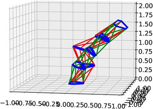
FIGURE 4. An example of a goal pose with two very different locally optimal solutions in IPOPT, for the Assembler defined in Section 5 with a 5 kg weight on the top plate. The red pose has a maximum leg force of 703N, while the green pose has a maximum leg force of only 282N. Axes units are in meters.

Moreover, to demonstrate the potentially high number of locally optimal solutions, we optimized the 2-SP Assembler with a goal pose of p = [0,0,0.65]^⊤ and r = [0,0,0]^⊤, so that a vertical pose is impossible due to the leg length lower-bounds. Using 100 randomized starting poses for the middle plate drawn from a normal distribution, and minimizing the maximal leg forces via IPOPT, we obtained 22 different locally optimal solutions, with maximum leg forces ranging from 457N to 519N.

2.6 Justification of four SPs in a stack

We choose the number of chained SP’s for an Assembler so that it can reach a ‘bent-over’ pose, with the end effector is in-plane with the bottom plate, facing downwards. This enables the assembler roughly a hemisphere of motion, allowing a reasonably large workspace while keeping internal forces under control. While adding additional SP’s would increase the kinematic flexibility of motion in a zero-gravity environment, on Earth, it would also increase the loads on the legs particularly for the bottom SP, thereby shrinking the workspace of the Assembler due to excessive forces.

For the specifications of the SP used in this work, due to leg length and joint motion limitations, a minimum of four chained SP’s are required to reach this bent-over pose. Thus, we use four chained SP’s for the computational tests in this work.

3 Assembler IK optimization

3.1 Definitions

In this section, we formally define the notation used for variables and parameters needed for this work.

Sets

To reduce notation definitions, we implicitly define some coordinate variables p, rotational variables r, and matrix variables R and T from ϒ via (2). We first define the sets of plates, SP’s, and legs per SP in the table below.

Parameters

Note that, as the Assembler studied in this work consists of N_P identical stacked SPs, there are really 2 plates between consecutive sets of legs, so that $m_i^P=2m_0^P=2m_{N_P}^P$ for i = 1, 2, …, N_P − 1. The problem variables and parameters are defined in their respective tables.

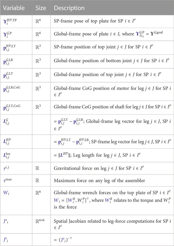
Variables

We assume that the Assembler is oriented so that gravity pulls directly downward in the reference frame of the Assembler, i.e., g = [0,0,−g]^⊤. To handle different orientations of the Assembler, one needs only to redefine the gravity vector g. Note that each ϒ transformation term implicitly defines corresponding TAA-form terms p and r, and matrix-form terms R and T. Finally, as the bottom plate is positioned at the origin of the global reference frame, we enforce that ${\mathbf{\Upsilon }}_0^{\mathcal{G},\text{P}}={\mathbf{\Upsilon }}_0^{\mathcal{G},\text{P},\text{rest}}=\mathbb{0}$.

In order to define a kinematically valid Assembler pose, we enforce the SP-frame kinematic validity constraints constraints in Section 2.4 for each SP, combined with the definition ${\mathbf{\Upsilon }}_{N_P}^{\mathcal{G},\text{P}}={\mathbf{\Upsilon }}^{\mathcal{G},\text{goal}}$, which ensures that the end-effector is where it should be.

This constraint is enforced with a small implicit tolerance within the nonlinear solver.

3.2 Force calculation

Force analysis follows the procedures set out in (Lynch and Park, 2017) with a few additional considerations.

For SP i ∈ I^P, we can define the Jacobian with the relationship

${J^{\text{s}}}_i^{-1}={\left[\begin{array}{ccc}\hfill {\mathbf{p}}_{i,1}^{\mathcal{G},\text{LB}}\times {\widehat{\mathit{L}}}_{i,1}^{\mathcal{G}}\hfill & \hfill \dots \hfill & \hfill {\mathbf{p}}_{i,6}^{\mathcal{G},\text{LB}}\times {\widehat{\mathit{L}}}_{i,6}^{\mathcal{G}}\hfill \\ \hfill {\widehat{\mathit{L}}}_{i,1}^{\mathcal{G}}\hfill & \hfill \dots \hfill & \hfill {\widehat{\mathit{L}}}_{i,6}^{\mathcal{G}}\hfill \end{array}\right]}^{\top }(13)$

where ${\widehat{\mathit{L}}}_{i,j}^{\mathcal{G}}$ is the unit vector for ${\mathit{L}}_{i,j}^{\mathcal{G}}$.

Given a wrench W defined in the global frame and acting on the SP end effector, the resultant forces on each of the SP’s legs can be determined by the relation:

${\mathit{\tau }}_{i,\left[1:6\right]}={\left({J^{\text{s}}}_i\right)}^{\top }{\left(\mathrm{A}\mathrm{d}\mathrm{j}\left({\mathbf{T}}_i^{\mathcal{G},\text{TP}}\right)\right)}^{\top }{W}_i(14)$

where, as in (Lynch and Park, 2017), we define the matrix adjoint for a transformation matrix T [see (4)] as

$\mathrm{A}\mathrm{d}\mathrm{j}\left(\mathbf{T}\right)≔\left[\begin{array}{cc}\hfill \mathbf{R}\hfill & \hfill \mathbb{0}\hfill \\ \hfill \left[\mathbf{p}\right]\mathbf{R}\hfill & \hfill \mathbf{R}\hfill \end{array}\right](15)$

For wrench computations, we first define the center of gravity for the motor and shaft of each leg j ∈ J for SP i ∈ I^P as

$\begin{array}{c}\hfill {\mathbf{p}}_{i,j}^{\mathcal{G},\text{LB},\text{CoG}}=d^{\text{LB},\text{CoG}}\frac{{\mathit{L}}_{i,j}^{\mathcal{G},\text{LT}}}{\Vert {\mathit{L}}_{i,j}^{\mathcal{G},\text{LT}}\Vert }+{\mathbf{p}}_{i,j}^{\mathcal{G},\text{LB}}\text{\hspace{0.17em}and\hspace{0.17em}}{\mathbf{p}}_{i,j}^{\mathcal{G},\text{LT},\text{CoG}}=d^{\text{LT},\text{CoG}}\frac{-{\mathit{L}}_{i,j}^{\mathcal{G},\text{LT}}}{\Vert {\mathit{L}}_{i,j}^{\mathcal{G},\text{LT}}\Vert }+{\mathbf{p}}_{i,j}^{\mathcal{G},\text{LT}}.\end{array}(16)$

Then, to compute the global-frame wrenches W_i for each SP, we sum all the wrenches from forces applied on or above the platform by leg masses, platform masses, and the end effector load. For i = 0, …, N_P − 2, this is computed as

$W_i=W_{i+1}+m_{i+1}^P\left[\begin{array}{c}\hfill \left[{\mathbf{p}}_{i+1}^{\mathcal{G},\text{P}}\right]\mathbf{g}\hfill \\ \hfill \mathbf{g}\hfill \end{array}\right]+{\displaystyle \sum _j}\left(m^{\text{LT}}\left[\begin{array}{c}\hfill \left[{\mathbf{p}}_{i+1,j}^{\mathcal{G},\text{LT},\text{CoG}}\right]\mathbf{g}\hfill \\ \hfill \mathbf{g}\hfill \end{array}\right]+m^{\text{LB}}\left[\begin{array}{c}\hfill \left[{\mathbf{p}}_{i+1,j}^{\mathcal{G},\text{LB},\text{CoG}}\right]\mathbf{g}\hfill \\ \hfill \mathbf{g}\hfill \end{array}\right]\right).(17)$

For the last platform i = N_P − 1, this is computed as

$\begin{array}{c}\hfill W_{N_P-1}=W^{\text{EE}}+m_{N_P}^P\left[\begin{array}{c}\hfill \left[{\mathbf{p}}_{N_P}^{\mathcal{G},T}\right]\mathbf{g}\hfill \\ \hfill \mathbf{g}\hfill \end{array}\right].\hfill \end{array}(18)$

Note that, as g = (0,0,−g)^⊤, for any vector $\mathbf{p}\in {\mathbb{R}}^3$, we have

$\left[\mathbf{p}\right]\mathbf{g}=g\left[\begin{array}{c}\hfill -{\mathbf{p}}_{\left[1\right]}\hfill \\ \hfill {\mathbf{p}}_{\left[2\right]}\hfill \\ \hfill 0\hfill \end{array}\right].$

Consequently, as W^EE is a parameter, and since the 3rd component of [p]g is zero, the 3rd-6th components of the wrench are known constants, while the first two depend linearly on the plate and leg locations.

3.3 IK heuristics

In this section, we introduce two heuristics for the initialization of SP poses.

3.3.1 Spline-based IK

In this section, we introduce a splined kinematic approach, denoting a cubic spline originating at the platform base plate and ending at the end effector position. Define the following positions as helper points ${\mathbf{p}}^{\mathcal{G},1}$ and ${\mathbf{p}}^{\mathcal{G},2}$ from the formulas:

${\mathbf{T}}^{\mathcal{G},1}≔{\mathbf{T}}^{\text{goal}}\left(-\frac{2}{3}{\mathbf{T}}_0^{\mathcal{T}\mathcal{P},\text{BP},\text{rest}}\right),{\mathbf{T}}^{\mathcal{G},2}≔{\mathbf{T}}^{\text{Base}}\left(\frac{2}{3}{\mathbf{T}}_{N_P}^{\mathcal{T}\mathcal{P},\text{BP},\text{rest}}\right).(19)$

Define the B-spline $p:[\mathrm{0,1}]\to {\mathbb{R}}^3$ as

$p\left(x\right)≔\mathrm{S}\mathrm{p}\mathrm{l}\mathrm{i}\mathrm{n}\mathrm{e}\left({\mathbf{p}}^{\mathcal{G},\text{Base}},{\mathbf{p}}^{\mathcal{G},1},{\mathbf{p}}^{\mathcal{G},2},{\mathbf{p}}^{\mathcal{G},\text{goal}}\right).(20)$

We use SciPy’s B-spline interpolation (Virtanen et al., 2020), which requires a minimum of four points to produce the spline curve, these two helper points serve a dual purpose: ensure that spline function has enough input to produce the expected curve, and also to ensure that interior plates are placed behind the plane of the goal end effector, and above the plane of the base plate. The resulting spline function provides the positions of the interior N_P − 1 plates via interpolation at ${\mathbf{p}}_i^{\mathcal{G},\text{P}}=p\left(\frac{i}{N_P}\right),$ for i = 0, 1, …, N_P. See Figure 5.

FIGURE 5

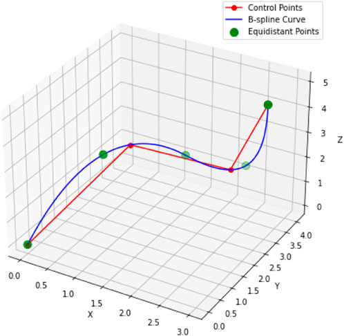
FIGURE 5. Possible example of calculation of plate centers ${\mathbf{p}}_i^{\mathcal{G},\text{P}}$ via the B-Spline calculation. Base plate and top plate locations are given, then control points are computed by transforming the base plate and top plate locations towards the rest pose. The B-spline is calculated, and then plate locations are determined as equidistant spacing along the spline.

We then recursively determine the rotation of the middle-most plate, and when there is an even number of plates left in the queue, we consider the two middle-most plates. The rotation of the middle-most plate(s) is then determined by an average of the rotation between the beginning and end plates, computed in TAA form in the reference frame of the beginning plate. Once the middle plate(s) rotation is determined, we recurse and determine the rotation of the next middle plate(s).

Within this heuristic, we consider a pose to be valid if all kinematic validity constraints, including the end-effector position, are satisfied within some small tolerance. If a pose fails kinematically, we attempt several recourse steps to correct the pose. In the event of failure (such as a calculated leg being too long), all legs are re-scaled such that the legs are within bounds, maintaining orientation, and the end effector position is recalculated accordingly.

Validation of the SP proceeds in steps, described in the following algorithm.

3.3.2 Same-SP initialization

We derive a simple initial guess for the Assembler pose by assuming that each SP has the same SP-frame pose ${\mathbf{\Upsilon }}_i^{\mathcal{B}\mathcal{P},\text{TP}}=\mathbf{\Upsilon }$. It is then trivial to compute the SP-frame rotation matrices, as since all share the same axis of rotation, we have for two rotations ${\mathbf{r}}_i^{BP,TP}$ and ${\mathbf{r}}_j^{BP,TP}$ that

${\mathbf{R}}_i^{\text{BP},\text{TP}}{\mathbf{R}}_j^{\text{BP},\text{TP}}=e^{\left[{\mathbf{r}}_i^{BP,TP}\right]}{e}^{\left[{\mathbf{r}}_j^{BP,TP}\right]}=e^{\left[{\mathbf{r}}_i^{BP,TP}+{\mathbf{r}}_j^{BP,TP}\right]}.$

Thus, if ${\mathbf{R}}_i^{\text{BP},\text{TP}}=\mathbf{R}$ for all i ∈ I^P, we obtain

${\mathbf{R}}_{N_P}^{\mathcal{G},\text{P}}=e^{\left[{\mathbf{r}}_{N_P}^{\mathcal{G},P}\right]}=e^{\left[N_P\mathbf{r}\right]}={\mathbf{R}}^{N_P}.$

Thus, we simply compute r as

$\mathbf{r}=\frac{1}{N_P}{\mathbf{r}}_{N_P}^{\mathcal{G},P}.$

Next, to compute the shared translation vector p, we first note that

${\mathbf{R}}_i^{\mathcal{G},\text{P}}={\mathbf{R}}^i$

and

$\begin{array}{cc}\hfill {\mathbf{p}}_1^{\mathcal{G},\text{P}}& =\mathbf{p}\hfill \\ \hfill {\mathbf{p}}_2^{\mathcal{G},\text{P}}& ={\mathbf{p}}_1^{\mathcal{G},\text{P}}+{\mathbf{R}}_1^{\mathcal{G},\text{P}}\mathbf{p}=\left({\mathbb{I}}^3+\mathbf{R}\right)\mathbf{p}\hfill \\ \hfill {\mathbf{p}}_3^{\mathcal{G},\text{P}}& ={\mathbf{p}}_2^{\mathcal{G},\text{P}}+{\mathbf{R}}_2^{\mathcal{G},\text{P}}\mathbf{p}=\left({\mathbb{I}}^3+\mathbf{R}+{\mathbf{R}}^2\right)\mathbf{p}\hfill \\ \hfill {\mathbf{p}}_i^{\mathcal{G},\text{P}}& =\left({\displaystyle \sum _{l=0}^{i-1}}{\mathbf{R}}^l\right)\mathbf{p}\hspace{1em}\hspace{1em}i\in I,\hfill \end{array}$

where ${\mathbb{I}}^3$ is the 3 × 3 identity matrix, and notable that ${\mathbf{R}}^0={\mathbb{I}}^3$ for any invertible 3 × 3 matrix R. We then obtain p via a single cheap linear solve. To summarize, we compute r and p, and the resulting ${\mathbf{R}}_i^{\mathcal{G},\text{P}}$ and ${\mathbf{p}}_i^{\mathcal{G},\text{P}}$’s, via

$\begin{array}{cc}\hfill \mathbf{r}& =\frac{1}{N_P}{\mathbf{r}}_{N_P}^{\mathcal{G},P}\hfill \\ \hfill \mathbf{R}& =e^{\left[\mathbf{r}\right]}\hfill \\ \hfill {\mathbf{p}}^{\mathcal{G},\text{P},\text{goal}}& =\left({\displaystyle \sum _{i=0}^{N_P-1}}{\mathbf{R}}^i\right)\mathbf{p}\hfill \\ \hfill {\mathbf{R}}_i^{\mathcal{G},\text{P}}& ={\mathbf{R}}^i\hspace{1em}\hspace{1em}i\in I\hfill \\ \hfill {\mathbf{p}}_i^{\mathcal{G},\text{P}}& =\left({\displaystyle \sum _{l=0}^{i-1}}{\mathbf{R}}^l\right)\mathbf{p}\hfill & i\in I\hfill \end{array}(21)$

where, again, p is computed via a linear solve in the third equation. Note that this initialization can correspond to multiple solutions, as e.g., a 180-degree z-rotation can be achieved via four 45-degree or four −45-degree z-rotations. Some examples of this phenomenon are shown in Figure 6. As such, we try up to two solutions in TAA form. Given ${\mathbf{\Upsilon }}_0^{\mathcal{G},\text{goal}}$, we first normalize $\Vert {\mathbf{r}}_0^{\mathcal{G},\text{goal}}\Vert$ to ensure $\Vert {\mathbf{r}}_0^{\mathcal{G},\text{goal}}\Vert <2\pi$. To this end, if $\Vert {\mathbf{r}}_0^{\mathcal{G},\text{goal}}\Vert \in \left[2k\pi ,2(k+1)\pi \right)$ for some integer k ≥ 1, we apply

${\mathbf{r}}_0^{\mathcal{G},\text{goal}}\leftarrow {\mathbf{r}}_0^{\mathcal{G},\text{goal}}\frac{\Vert {\mathbf{r}}_0^{\mathcal{G},\text{goal}}\Vert -2k\pi }{\Vert {\mathbf{r}}_0^{\mathcal{G},\text{goal}}\Vert }.$

FIGURE 6

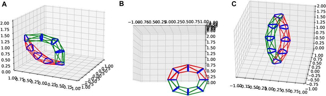
FIGURE 6. Some examples of pose initialization results. The red poses are the originals, while the green poses are reflected. (A) First try yields extreme angles and flattened SP’s; (B) reflected try yields inverted pose with legs clipping through the plates; (C) initializations yield mirrored poses. Axes units are in meters.

Then, if we find that the resulting SP-frame translation vector ${\mathbf{p}}^{\mathcal{B}\mathcal{P},\text{TP}}$ is too far (more than 60°) from vertical, which is true if and only if

${\mathbf{p}}_{\left[2\right]}\le \Vert \mathbf{p}\Vert \cos \left(\frac{\pi }{3}\right),$

we reject the solution, and then try a second one. We obtain this second solution by reflecting the rotation $\Vert {\mathbf{r}}_0^{\mathcal{G},\text{goal}}\Vert$ about π to achieve the same rotation from the opposite direction, via

${\mathbf{r}}_0^{\mathcal{G},\text{goal}}\leftarrow {\mathbf{r}}_0^{\mathcal{G},\text{goal}}\frac{2\pi -\Vert {\mathbf{r}}_0^{\mathcal{G},\text{goal}}\Vert }{\Vert {\mathbf{r}}_0^{\mathcal{G},\text{goal}}\Vert }.$

We have found computationally that this procedure consistently yields useful initial guesses for the optimizer, though the guesses are often kinematically invalid.

3.4 Force-based IK optimization

We formulate the optimization problem for a stacked SP Assembler as a quadratically constrained quadratic program (QCQP). In this model, ${\mathbf{R}}_i^{\mathcal{G},\text{P}}$ and ${\mathbf{p}}_i^{\mathcal{G},\text{P}}$ are the driving decision variables, in that they uniquely specify a pose. The rest of the variables are derived directly from these. Note that, due to our choice of reference frame, we have ${\mathbf{R}}_0^{\mathcal{G},\text{P}}=e^{[\mathbb{0}]}={\mathbb{I}}^3$, where ${\mathbb{I}}^3$ is the 3 × 3 identity matrix.

Constraints related to kinematic validity are denoted via (KVC); all other constraints establish definitions of intermediate variables.

Equations in this section are either labeled as (M#) to denote that they are used explicitly in the model, or as (#), to denote that this is just a calculation useful to deriving the model equations.

3.4.1 Additional definitions

For the optimization model, we use all variables and parameters in Section 3.1 except $J_i^{\text{s}}$, including only R and p for each ϒ variable or parameter, and add the following additional variables. For clearer distinction between variables and parameters within this model, we will represent all variables using $\text{blue}$ text.

3.4.2 Constraints

Vector Norms: To model the two-norm $\Vert {\mathit{L}}_{i,j}^{\mathcal{B}\mathcal{P}}\Vert$ of the leg length vector (which is equivalent to $\Vert {\mathit{L}}_{i,j}^{\mathcal{G}}\Vert$), we introduce intermediate variable ${\mathit{L}}_{i,j}^{\mathrm{l}\mathrm{e}\mathrm{n}}$, then add the constraint

${\mathit{L}}_{i,j}^{\mathrm{l}\mathrm{e}\mathrm{n}2}={\displaystyle \sum _{k=1}^3}{\mathit{L}}_{i,j,[k]}^2\forall i\in I^P,j\in J.(\mathrm{M1})$

$\Vert \mathit{v}{\Vert }^2={\displaystyle \sum _{k=1}^m}{\mathit{v}}_{\left[k\right]}^2,(\mathrm{22a})$

$\Vert \mathbf{R}{\Vert }_F^2={\displaystyle \sum _{k=1}^m}{\displaystyle \sum _{l=1}^m}{\mathbf{R}}_{\left[k,l\right]}^2.(\mathrm{22b})$

Reference Frame Computations: The constraints in this section are needed to define ${\mathbf{R}}_i^{\text{BP},\text{TP}}$’s and ${\mathbf{R}}_i^{\mathcal{G},\text{P}}$’s. First, we express the global rotation matrices via their columns as

${\mathbf{R}}_i^{\mathcal{G},\text{P}}=\left[\left.{\mathbf{R}}_{i,[:,1]}^{\mathcal{G},\text{P}}\right|{\mathbf{R}}_{i,[:,2]}^{\mathcal{G},\text{P}}\left|{\mathbf{R}}_{i,[:,3]}^{\mathcal{G},\text{P}}\right.\right]i\in I.(\mathrm{M2})$

Note that, as rotation matrices define an orthonormal right-handed coordinate system, it is sufficient to consider ${\mathbf{R}}_{i,[:,1]}^{\mathcal{G},\text{P}}$ and ${\mathbf{R}}_{i,[:,2]}^{\mathcal{G},\text{P}}$ as the driving variables, then compute ${\mathbf{R}}_{i,[:,3]}^{\mathcal{G},\text{P}}$ as

${\mathbf{R}}_{i,[:,3]}^{\mathcal{G},\text{P}}={\mathbf{R}}_{i,[:,1]}^{\mathcal{G},\text{P}}\times {\mathbf{R}}_{i,[:,2]}^{\mathcal{G},\text{P}}.(\mathrm{M3})$

We then ensure the orthonormality of each ${\mathbf{R}}_{i,[:,1]}^{\mathcal{G},\text{P}}$ and ${\mathbf{R}}_{i,[:,2]}^{\mathcal{G},\text{P}}$ via

$\begin{array}{cc}\hfill {‖{\mathbf{R}}_{i,[:,1]}^{\mathcal{G},\text{P}}‖}^2& =1,\hfill \\ \hfill {‖{\mathbf{R}}_{i,[:,2]}^{\mathcal{G},\text{P}}‖}^2& =1,\hfill \\ \hfill {\mathbf{R}}_{i,[:,1]}^{\mathcal{G},\text{P}}\cdot {\mathbf{R}}_{i,[:,2]}^{\mathcal{G},\text{P}}& =0.\hfill \end{array}(\mathrm{M4})$

Next, to obtain the translation portion of each plate transformation in the SP frame, we inverse transform the global-frame point ${\mathbf{p}}_i^{\mathcal{G}}$ by ${\mathbf{T}}_i^{\mathcal{G}}$ by solving the forward transformation ${\mathbf{p}}_i^{\mathcal{G}}={\mathbf{T}}_i^{\mathcal{G}}\diamond {\mathbf{p}}_i^{\mathcal{B}\mathcal{P},\text{TP}}$, as defined in (5), for the pre-transformed point ${\mathbf{p}}_i^{\mathcal{B}\mathcal{P},\text{TP}}$, yielding

$\begin{array}{ccc}\hfill {\mathbf{p}}_i^{\mathcal{B}\mathcal{P},\text{TP}}& ={({\mathbf{R}}_i^{\mathcal{G},\text{P}})}^{\top }({\mathbf{p}}_{i+1}^{\mathcal{G},\text{P}}-{\mathbf{p}}_i^{\mathcal{G},\text{P}})\hfill & i\in I^P.\hfill \end{array}(\mathrm{M5})$

We constrain that the bottom plate is at the origin in the global Assembler frame via

$\begin{array}{cc}\hfill {\mathbf{p}}_0^{\mathcal{G},\text{P}}& =\mathbb{0}\hfill \\ \hfill {\mathbf{R}}_0^{\mathcal{G},\text{P}}& ={\mathbb{I}}^3.\hfill \end{array}(\mathrm{M6})$

Finally, we define the SP-frame rotation matrices ${\mathbf{R}}_i^{\text{BP},\text{TP}}$ via ${\mathbf{R}}_i^{\mathcal{G},\text{P}}{\mathbf{R}}_i^{\text{BP},\text{TP}}={\mathbf{R}}_{i+1}^{\mathcal{G},\text{P}}$, yielding

$\begin{array}{cc}\hfill {\mathbf{R}}_i^{\text{BP},\text{TP}}={\left({\mathbf{R}}_i^{\mathcal{G},\text{P}}\right)}^{\top }{\mathbf{R}}_{i+1}^{\mathcal{G},\text{P}}& i\in I^P.\hfill \end{array}(\mathrm{M7})$

Moreover, any expressions of the form ‖v‖², $\mathit{v}\in {\mathbb{R}}^m$, or $\Vert \mathbf{R}{\Vert }_F^2$, $\mathbf{R}\in {\mathbb{R}}^{m\times m}$, as in (M4), (T4), and (T1), are substituted explicitly with the defining expressions.

Leg Attachment Locations: In (M8), we define the SP-frame and global-frame locations of the leg attachments on the top/bottom plates for each SP according to (6). Note that the position of the bottom leg attachments are known constants in local space. See also Figure 3.

$\begin{array}{ccc}\hfill {\mathbf{p}}_{i,j}^{\mathcal{B}\mathcal{P},\text{LT}}& ={\mathbf{R}}_i^{\text{BP},\text{TP}}{\mathbf{p}}_{i,j}^{\mathcal{T}\mathcal{P},\text{LT},\text{rest}}+{\mathbf{p}}_i^{\mathcal{B}\mathcal{P},\text{TP}}\hfill & \forall i\in I^P,j\in J\hfill \\ \hfill {\mathbf{p}}_{0,j}^{\mathcal{G},\text{LB}}& ={\mathbf{p}}_{0,j}^{\mathcal{G},B,\text{rest}}\hfill & \forall j\in J\hfill \\ \hfill {\mathbf{p}}_{i,j}^{\mathcal{G},\text{LB}}& ={\mathbf{R}}_i^{\mathcal{G},\text{P}}{\mathbf{p}}_{i,j}^{\mathcal{B}\mathcal{P},\text{LB}}+{\mathbf{p}}_i^{\mathcal{G}}\hfill & \forall i\in I^P,i\ge 1,j\in J\hfill \\ \hfill {\mathbf{p}}_{i,j}^{\mathcal{G},\text{LT}}& ={\mathbf{R}}_{i+1}^{\mathcal{G},\text{P}}{\mathbf{p}}_{i,j}^{\mathcal{T}\mathcal{P},\text{LT},\text{rest}}+{\mathbf{p}}_{i+1}^{\mathcal{G}}\hfill & \forall i\in I^P,j\in J.\hfill \end{array}(\mathrm{M8})$

Leg Centers of Gravity: To define the center of gravity for each leg j ∈ J for SP i ∈ I^P, we start with (16), multiply through by denominators, and rearrange, yielding

$\begin{array}{cc}\hfill {\mathit{L}}_{i,j}^{\mathrm{l}\mathrm{e}\mathrm{n}}({\mathbf{p}}_{i,j}^{\mathcal{G},\text{LB},\text{CoG}}-{\mathbf{p}}_{i,j}^{\mathcal{G},\text{LB}})& =d^{\text{LB},\text{CoG}}{\mathit{L}}_{i,j}^{\mathcal{G}},\hfill \\ \hfill {\mathit{L}}_{i,j}^{\mathrm{l}\mathrm{e}\mathrm{n}}({\mathbf{p}}_{i,j}^{\mathcal{G},\text{LT}}-{\mathbf{p}}_{i,j}^{\mathcal{G},\text{LT},\text{CoG}})& =d^{\text{LT},\text{CoG}}{\mathit{L}}_{i,j}^{\mathcal{G}}.\hfill \end{array}(\mathrm{M9})$

Leg Length Bounds: (KVC) We define the leg length bounding constraints via (8), as

$L^{\min }\le {\mathbf{L}}_{i,j}^{\mathrm{l}\mathrm{e}\mathrm{n}}\le L^{\max }.(\mathrm{M10})$

Note that the upper-bounding leg length constraints are second order cone constraints in terms of ${\mathbf{p}}_i^{\mathcal{B}\mathcal{P},\text{TP}}$ and ${\mathbf{R}}_i^{\mathcal{B}\mathcal{P},\text{TP}}$ (as the interiors of spheres), while the lower-bounding constraints are nonconvex as sphere exteriors.

Leg Angle Deviation: (KVC) The bottom-plate leg angle deviation constraints are defined via (9), after multplying through by denominators, as The bottom-plate leg angle deviation constraints are defined via (9), as

$\begin{array}{c}\hfill {\mathbf{L}}_{i,j}^{\mathrm{l}\mathrm{e}\mathrm{n}}\Vert {\mathit{L}}_{i,j}^{\mathcal{B}\mathcal{P},\text{rest}}\Vert \cos ({\theta }^{\max })\le {\mathbf{L}}_{i,j}^{\mathcal{B}\mathcal{P}}\cdot {\mathit{L}}_{i,j}^{\mathcal{B}\mathcal{P},\text{rest}}\forall i\in I^P,j\in J.\end{array}(\mathrm{M11})$

while the top-plate constraints are defined via (10), after multiplying through by denominators, as

$\begin{array}{c}\hfill {\mathbf{L}}_{i,j}^{\mathrm{l}\mathrm{e}\mathrm{n}}\Vert {\mathit{L}}_{i,j}^{\mathcal{B}\mathcal{P},\text{rest}}\Vert \cos ({\theta }^{\max })\le {\mathbf{L}}_{i,j}^{\mathcal{B}\mathcal{P}}\cdot ({\mathbf{R}}_i^{\text{BP},\text{TP}}{\mathit{L}}_{i,j}^{\mathcal{B}\mathcal{P},\text{rest}})\forall i\in I^P,j\in J.\end{array}(\mathrm{M12})$

Note that all leg angle deviation constraints are second-order cone constraints given fixed rotation matrices.

Continuous Translation Enforcement: (KVC) We enforce that legs do not break the surface of the bottom plate of any SP via (11), as

${\mathbf{p}}_{i,j,\left[3\right]}^{\mathcal{B}\mathcal{P},\text{LT}}\ge {\mathbf{p}}_{i,j,\left[3\right]}^{\mathcal{B}\mathcal{P},\text{LB}}(23)$

Extreme Pose Prevention: (KVC) To help prevent extreme and difficult-to-reach poses for each SP, we enforce (12), as

${\mathbf{R}}_{i,\left[k,k\right]}^{\text{BP},\text{TP}}\ge \cos \left({\theta }^{\mathbf{R},\max }\right),k=\mathrm{1,2,3}(24)$

End Effector: (KVC) We enforce that the end effector pose is exactly as desired via

$\begin{array}{c}\hfill {\mathbf{p}}_{N_P-1}^{\mathcal{G},\text{P}}={\mathbf{p}}^{\mathcal{G},\text{P}\text{goal}}\hfill \\ \hfill {\mathbf{R}}_{N_P-1,[:,1]}^{\mathcal{G},\text{P}}={\mathbf{R}}_{[:,1]}^{\mathcal{G},\text{P},\text{goal}}\\ \hfill {\mathbf{R}}_{N_P-1,[:,2]}^{\mathcal{G},\text{P}}={\mathbf{R}}_{[:,2]}^{\mathcal{G},\text{P},\text{goal}}\end{array}(\mathrm{M13})$

where ${\mathbf{p}}^{\mathcal{G},\text{P},\text{goal}}$ and ${\mathbf{R}}^{\mathcal{G},\text{P},\text{goal}}$ are computed from ${\mathbf{\Upsilon }}^{\mathcal{G},\text{goal}}$.

Objective: The objective is to minimize maximal leg force

$\min {\tau }^{\max }.(\mathrm{M14})$

where the constraints defining the maximum force τ^max are introduced in Section 3.4.3.

Initialization: As the model is solved only to local optimality via IPOPT due to the intractability of a global solve even with N_P = 2, an initial solution for the pose is required. We choose to initialize via the same-SP initialization scheme in Section 3.3.2, as it performed much better in our numerical testing when compared to the spline-based scheme in Section 3.3.1, despite yielding valid poses less often before optimization.

3.4.3 Forces

Referring to (15), the transposed adjoint of a transformation matrix T is

$\mathrm{A}\mathrm{d}\mathrm{j}{\left(\mathbf{T}\right)}^{\top }=\left[\begin{array}{cc}\hfill {\mathbf{R}}^{\top }\hfill & \hfill {\mathbf{R}}^{\top }{\left[\mathbf{p}\right]}^{\top }\hfill \\ \hfill \mathbb{0}\hfill & \hfill {\mathbf{R}}^{\top }\hfill \end{array}\right].(25)$

For shorthand, we let ${\mathbf{A}}_i:=\mathrm{A}\mathrm{d}\mathrm{j}{\left({\mathbf{T}}_i^{\mathcal{G}}\right)}^{\top }$ for each i ∈ I.

Each column of the transposed inverse Jacobian $J^{\text{t}}$ as in (13) via (M15), can be computed as (see (Lynch and Park, 2017) for discussion on single SPs)

${\mathit{L}}_{i,j}^{\mathrm{l}\mathrm{e}\mathrm{n}}{J^{\text{t}}}_{i,[:,j]}=\left[\begin{array}{c}\hfill [{\mathbf{p}}_{i,j}^{\mathcal{G},\text{LB}}]{\mathit{L}}_{i,j}^{\mathcal{G}}\hfill \\ \hfill {\mathit{L}}_{i,j}^{\mathcal{G}}\hfill \end{array}\right]\forall i\in I^P,j\in J.(\mathrm{M15})$

Note that ${\mathit{L}}_{i,j}^{\mathrm{l}\mathrm{e}\mathrm{n}}=\Vert {\mathbf{p}}_{i,j}^{\mathcal{G},\text{LT}}-{\mathbf{p}}_{i,j}^{\mathcal{G},\text{LB}}\Vert =\Vert {\mathbf{p}}_{i,j}^{\mathcal{B}\mathcal{P},\text{LT}}-{\mathbf{p}}_{i,j}^{\mathcal{B}\mathcal{P},\text{LB}}\Vert$ is the length of the corresponding leg, as modelled in (M1).

To compute the global-frame wrenches for each SP, we use (17) for i = 0, …, N_P − 2 and (18) for i = N_P − 1.

Finally, to compute the leg forces, and defining ${\mathit{\tau }}_i={[{\mathit{\tau }}_{i,1},\dots ,{\mathit{\tau }}_{i,6}]}^{\top }$ for each i, we use the vector constraints

$\begin{array}{ccc}\hfill {J^{\text{t}}}_i{\mathit{\tau }}_i& ={\mathbf{A}}_i{W}_i\hfill & \forall i\in I^P\hfill \\ \hfill {\tau }^{\max }& \ge {\tau }_{i,j}\hfill & \forall i\in I^P,j\in J\hfill \\ \hfill {\tau }^{\max }& \ge -{\tau }_{i,j}\hfill & \forall i\in I^P,j\in J\hfill \end{array}(\mathrm{M16})$

where the jth component of the resulting solution ${\mathit{\tau }}_i$ is the force on the jth leg of the ith SP. We then minimize over $\tau$.

Notice that ${\mathbf{A}}_i{W}_i$ can be written as:

${\mathbf{A}}_i{W}_i=\left[\begin{array}{cc}\hfill {\left({\mathbf{R}}_i^{\mathcal{G},\text{P}}\right)}^{\top }\hfill & \hfill {\left({\mathbf{R}}_i^{\mathcal{G},\text{P}}\right)}^{\top }{\left[{\mathbf{p}}_i^{\mathcal{G},\text{P}}\right]}^{\top }\hfill \\ \hfill \mathbb{0}\hfill & \hfill {\left({\mathbf{R}}_i^{\mathcal{G},\text{P}}\right)}^{\top }\hfill \end{array}\right]\left[\begin{array}{c}\hfill W_i^R\hfill \\ \hfill W_i^P\hfill \end{array}\right]=\left[\begin{array}{c}\hfill {\left({\mathbf{R}}_i^{\mathcal{G},\text{P}}\right)}^{\top }\left(W_i^R+{\left[{\mathbf{p}}_i^{\mathcal{G},\text{P}}\right]}^{\top }{W}_i^P\right)\hfill \\ \hfill {\left({\mathbf{R}}_i^{\mathcal{G},\text{P}}\right)}^{\top }{W}_i^P\hfill \end{array}\right].$

Thus, the first constraint of (M16) is equivalent to, and implemented as,

$\begin{array}{cc}\hfill {J^{\text{t}}}_i{\mathit{\tau }}_i& =\left[\begin{array}{c}\hfill {({\mathbf{R}}_i^{\mathcal{G},\text{P}})}^{\top }(W_i^R+{[{\mathbf{p}}_i^{\mathcal{G},\text{P}}]}^{\top }{W}_i^P)\hfill \\ \hfill {({\mathbf{R}}_i^{\mathcal{G},\text{P}})}^{\top }{W}_i^P\hfill \end{array}\right]i\in I^P.\hfill \end{array}(\mathrm{M17})$

Note that this constraint is bilinear in nature, since $W_i^P$ is a constant.

If w₂ ≠ 0, we also enforce that the force on each leg does not exceed the maximum allowable force, via

$\begin{array}{c}\hfill {\tau }^{\max }\le f^{\max }\end{array}(\mathrm{M18})$

3.4.4 Improving robustness

Due to the nature of iterative local nonlinear optimization via e.g., IPOPT, the equality constraints defining various intermediate variables such as leg lengths, rotation matrices, the inverse Jacobian etc., and even primary constraints such as end-effector position, can become violated as the solver attempts to resolve violations of the physical constraints defining a valid pose. We have observed that this can sometimes lead to instability within the optimizer, particularly if the end effector is moved from the goal position during optimization.

To address this instability while controlling for computational time, we implement an iterative-refinement scheme around the basic nonlinear optimizer. Here, we leverage the fact that the variables ${\mathbf{\Upsilon }}_i^{\mathcal{G},\text{P}}$ uniquely define the Assembler. Thus, if an optimization seems to be converging slowly or returns with a ‘locally infeasible’ status, we re-initialize the model every so often, and reset the end effector to the correct location.

To this end, we set the maximum total internal iteration count as 2,500. Every k iterations, if the solver has not yet converged, we stop the solve, re-initialize using the plate locations and corrected the end effector location, then continue. We start with k = 500, but for each internal solver error we divide k in half and try again, with up to five such retries.

Occasionally, locally infeasible solutions can occur at valid poses, due to numerical difficulties in resolving force-related equality constraints. This results in sub-optimal, but kinematically valid, poses. When using IPOPT as the nonlinear solver, we have observed that the solver can often recover from such poses after re-initialization. Thus, to handle this contingency, on the first consecutive ‘locally infeasible’ result, we deduct k iterations from the remaining total (as if the solver had run k iterations) and re-initialize as usual. On the second consecutive locally infeasible result for the same pose, we report an optimization failure due to local infeasibility within the solver.

4 Trajectory planning

The Assembler is designed to be a movable platform that can help with complicated operations. As such, it is important that it can move from one position to another. We will adapt the tools in the prior section to develop trajectory optimization techniques. We present two approaches: a naïve direct transformation and a force optimization using trust regions. We also implemented an RRT* version that hinges on sub-paths computed from the force optimization approach. However, our RRT* did not produce as good results as the trust region method, so we do not include that in our description or results here.

Equations in this section are either labeled as (N#) (T#), or (#) to denote equations for naïve method, trust method, or calculations, respectively.

4.1 Naïve direct transformation

We establish the simplest approach to move from one pose to another that we call the naïve method. This approach is ignorant to force calculations, and thus is very prone to generating infeasible trajectories that violate the maximum force bounds. The approach simply uses a linear interpolation of the vector of leg lengths throughout the motion. For each target leg-length vector ${\mathit{L}}_{i,j}^{\text{goal}}$, i ∈ I^P, j ∈ J, the FK problem is solved to obtain the full trajectory planning solution. To solve this problem, we first attempt the widely-used Newton-Raphson approach, as in e.g., (Nguyen and Antrazi, 1990; Merlet, 2006). If this does not succeed, we then leverage a force-free version of the nonlinear optimizer to solve the FK problem, in which the end effector is allowed to move, and we optimize the squared leg-length-distance from the goal. More formally, to construct a QCQP model for the FK problem, we begin with the model in Section 3.4, then remove all force-related constraints and the end effector constraint (M13). We then optimize

$\min {\displaystyle \sum _{i\in I^P}}{\displaystyle \sum _{j\in J}}{({\mathbf{L}}_{i,j}-{\mathit{L}}_{i,j}^{\text{goal}})}^2.(\mathrm{N1})$

Note that the FK problem for the Assembler can decompose into separate FK problems for each SP.

4.2 Trust region optimization

We introduce a trust region method for trajectory planning of the SP. This algorithm first optimizes the starting and goal poses, then iteratively tries to make small steps towards the goal pose until it is sufficiently close, while trying to maintain forces that do not exceed those in the starting or ending poses.

4.2.1 Additional definitions

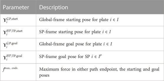
To define the optimization problem for a single step, we first introduce the following additional parameters for the full optimization.

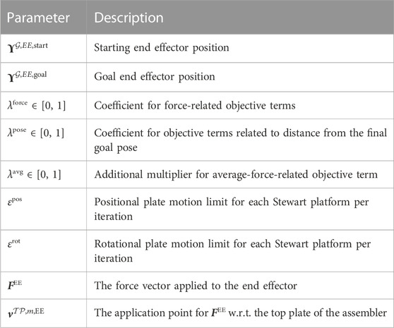
Additional parameters for trajectory planning problem.

Note that we normalize the non-negative objective weights with λ^force + λ^pose = 1. We then compute the full optimized starting and ending poses by solving the QCQP model in Section 3.4 with IPOPT, then compute the maximum force observed in either pose.

Computed initial state parameter for trajectory planning problem.

Note that, for practical use, the starting pose would be specified directly as the current pose of the Assembler.

For each iteration, we define the pose from the previous iteration as

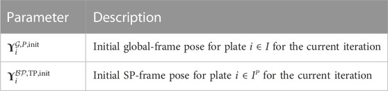
Initial state parameters for the current iteration of the trust region trajectory planning method.

Finally, we introduce the following additional variables for each iteration.

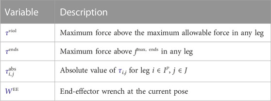
Additional variables for the current iteration of the trust region trajectory planning method.

4.2.2 Constraints

We begin with the model in Section 3.4, omitting the end effector constraints (M13) and the explicit force constraint (M18). We also redefine the end effector wrench definition W^EE to account for the fact that the end effector is no longer at a fixed position.

We then add constraints to ensure that no plate moves a distance further than ɛ^pos from ${\mathbf{p}}_i^{\mathcal{G},P,\text{init}}$, measured in two-norm, and rotates no further than ɛ^rot from ${\mathbf{R}}_i^{\mathcal{G},\text{P},\text{init}}$, measured in matrix Frobenius norm. The Frobenius norm was chosen for its superior performance and robustness compared to more direct angle-based measures in preliminary testing, combined with its simplicity and convexity. Finally, we add constraints to define τ^viol and τ^ends, then define the objective function.

Motion Limit: We ensure that positional and rotational motions are sufficiently controlled via

$\begin{array}{ccc}\hfill \Vert {\mathbf{R}}_i^{\mathcal{G},\text{P}}-{\mathbf{R}}_i^{\mathcal{G},\text{P},\text{init}}{\Vert }_F^2& \le {\left({\epsilon }^{\text{rot}}\right)}^2\hfill & i\in I,i\ge 1\hfill \\ \hfill \Vert {\mathbf{R}}_i^{\mathcal{G},\text{P}}-{\mathbf{p}}^{\mathcal{G},\text{P},\text{init}}{\Vert }^2& \le {\left({\epsilon }^{\text{pos}}\right)}^2\hfill & i\in I,i\ge 1.\hfill \end{array}(\mathrm{T1})$

Force Definitions: To define wrenches, we first define the now-variable rotational component $W$^R,EE of the end effector wrench $W$^EE via

$\begin{array}{cc}\hfill {\mathbf{p}}^{\mathcal{G},m,\text{EE}}& ={\mathbf{R}}_{N_P}^{\mathcal{G},\text{P}}{\mathit{v}}^{\mathcal{T}\mathcal{P},m,\text{EE}}+{\mathbf{p}}_{N_P}^{\mathcal{G},\text{P}}\hfill \\ \hfill W^{R,\text{EE}}& =[{\mathbf{p}}^{\mathcal{G},m,\text{EE}}]{\mathit{F}}^{\text{EE}}\hfill \end{array}(\mathrm{T2})$

where the translational component W^P,EE = F^EE of the wrench is constant. We then use (18) and (17) to define plate wrenches as before. Next, we define the additional required force-related variables with

$\begin{array}{ccc}\hfill {\tau }^{\text{viol}}& \ge {\tau }^{\max }-f^{\max }\hfill & \forall i\in I^P,j\in J\hfill \\ \hfill {\tau }^{\text{ends}}& \ge {\tau }^{\max }-f^{\max ,\text{ends}}\hfill & \forall i\in I^P,j\in J\hfill \\ \hfill {\tau }_{i,j}^{\text{abs}}& \ge {\tau }_{i,j}\hfill & \forall i\in I^P,j\in J\hfill \\ \hfill {\tau }_{i,j}^{\text{abs}}& \ge -{\tau }_{i,j}\hfill & \forall i\in I^P,j\in J\hfill \\ \hfill {\tau }^{\text{viol}}& \ge 0\hfill \\ \hfill {\tau }^{\text{ends}}& \ge 0\hfill \end{array}(\mathrm{T3})$

Note that, through ${\tau }^{\text{viol}}$, the max-force constraints on the legs are moved to the objective with a high coefficient. For the purposes of balancing objective terms related to forces, distances, and rotation angles, we assume forces and distances are measured in SI units (i.e., Newtons and meters). Note that the rotation terms are unit-independent, as they are measured via Frobenius norms of unitary rotation matrices.

4.2.3 Objective

To assist in defining the objective functions, we define the following expressions for the sake of readability. These definitions are the ‘distance-to-goal’ metrics for the objective function

$\begin{array}{cc}\hfill {\tau }^{1-\text{norm}}& ={\displaystyle \sum _{i\in I^P}}{\displaystyle \sum _{j\in J}}{\tau }_{i,j}^{\text{abs}},\hfill \\ \hfill {\mathcal{E}}^{\text{pos}}& ={\displaystyle \sum _{i\in I^P}}\Vert {\mathbf{p}}_i^{\mathcal{B}\mathcal{P},\text{TP}}-{\mathbf{p}}_i^{\mathcal{B}\mathcal{P},\text{TP},\text{goal}}{\Vert }^2,\hfill \\ \hfill {\mathcal{E}}^{\text{rot}}& ={\displaystyle \sum _{i\in I^P}}\Vert {\mathbf{R}}_i^{\mathcal{B}\mathcal{P}}-{\mathbf{R}}_i^{\mathcal{B}\mathcal{P},\text{goal}}{\Vert }_F^2.\hfill \end{array}(\mathrm{T4})$

With these definitions, we define the objective function as

$\min {\lambda }^{\text{force}}({\tau }^{\text{ends}}+\frac{{\lambda }^{\text{avg}}}{6N_P}{\tau }^{1-\text{norm}}+1000{\tau }^{\text{viol}})+{\lambda }^{\text{pose}}({\mathcal{E}}^{\text{pos}}+\frac{1}{4}{\mathcal{E}}^{\text{rot}}).(\mathrm{T5})$

Note that the decision to divide the ${\mathcal{E}}^{\text{rot}}$ by 4 serves to balance the position and rotation distance metrics, and performed well in preliminary testing compared to other coefficients. For Assemblers consisting of SP’s of different sizes, this divisor should be re-scaled according to the size of the SP, while the choice of λ^force should be re-scaled according to the weight of the SP.

4.2.4 Iteration

The trust region method proceeds by solving the problem described above until convergence. However, the process often stagnates, reaching positions where the objective to reduce forces overrides the objective to move towards the goal pose, or even moves in the wrong direction to improve average forces. When stagnation occurs due to high maximum forces, we divide λ^force by 2, set λ^pose = 1 − λ^force, and try again with the same initial positions. Similarly, if either stagnation or motion in the wrong direction occurs due to average forces, we divide λ^avg by 4 and try again with the same initial positions. The method converges when the distance between the current pose and the goal pose is small enough that the goal pose is a valid solution for the next iteration.

More formally, for the current iteration, define

$\begin{array}{c}\hfill {\mathcal{E}}^{\max ,\text{pos}}=\underset{i\in I,i\ge 1}{\max }\Vert {\mathbf{p}}_i^{\mathcal{G},\text{P},\text{init}}-{\mathbf{p}}^{\mathcal{G},\text{P},\text{goal}}\Vert ,\\ \hfill {\mathcal{E}}^{\max ,\text{rot}}=\underset{i\in I,i\ge 1}{\max }\Vert {\mathbf{R}}_i^{\mathcal{G},\text{P},\text{init}}-{\mathbf{R}}_i^{\mathcal{G},\text{P},\text{goal}}{\Vert }_F.\end{array}(26)$

Then convergence occurs when both ${\mathcal{E}}^{\max ,\text{pos}}\le {\epsilon }^{\text{pos}}$ and ${\mathcal{E}}^{\max ,\text{rot}}\le {\epsilon }^{\text{rot}}$. Early termination occurs if the process has stagnated or moved in the wrong direction too many times, or if too many iterations have been reached.

Due to the multi-objective nature of the trust region method, it is possible that insufficient progress towards the goal can occur during the solve. We call this a stagnation and formally define this to occur when one of the following criteria are met after optimizing:

$\begin{array}{c}\hfill \underset{i\in I,i\ge 1}{\max }\Vert {\mathbf{p}}_i^{\mathcal{G},\text{P}}-{\mathbf{p}}^{\mathcal{G},\text{P},\text{init}}\Vert \le \frac{{\epsilon }^{\text{pos}}}{100},\\ \hfill \underset{i\in I,i\ge 1}{\max }\Vert {\mathbf{R}}_i^{\mathcal{G},\text{P}}-{\mathbf{R}}_i^{\mathcal{G},\text{P},\text{init}}{\Vert }_F\le \frac{{\epsilon }^{\text{rot}}}{100}.\end{array}(27)$

Even if λ^avg = 0, stagnation can occur in the optimizer if $\tau$ ^max = f ^{max, ends} and further progress requires forces above f ^{max, ends}. Thus, if stagnation occurs, we conclude that the average-force term is the culprit only if $\tau$ ^max ≤ f ^{max, ends} − 0.001, where the 1 mN subtraction is added to be conservative, helping to prevent the algorithm from stagnating with repeated, futile reductions of λ^avg.

We define a step to be in the wrong direction if both the positional and rotational components of the motion have moved somewhat away from the goal pose, i.e., if for an iteration k we have ${\mathcal{E}}_k^{\max ,\text{pos}}\ge {\mathcal{E}}_{k-1}^{\max ,\text{pos}}+10^{-4}$ and ${\mathcal{E}}_k^{\max ,\text{rot}}\ge {\mathcal{E}}_{k-1}^{\max ,\text{rot}}+10^{-4}$. We allow motion in the wrong direction in order to reduce maximum leg forces that seemed excessive, i.e., if $\tau$ ^max > f ^{max, ends}. If we reject the motion step, then the position-related terms in the objective function have worsened while the max-force-related terms have not improved, and so the average force term must be the culprit.

Define the maximum allowed number of stagnated iterations as n^{max, stag}, and define the maximum number of iterations as k^max. The iteration then proceeds as in Algorithm 1. For shorthand, we define the solution path as a list of poses from the starting pose to the goal pose. As defined in Section 2, a pose is the corresponding list of ${\mathbf{p}}_i^{\mathcal{G},\text{P}}$’s and ${\mathbf{R}}_i^{\mathcal{G},\text{P}}$’s.

Algorithm 1. General procedure for trust-region trajectory planning method.

Input: A starting position pose^start and ending position pose^ends.

Output: An integer K and a sequence of poses pose₀, …, pose_k

1 n^stag ← 0, k ← 1, pose₀ ← pose^start

2 while not converged and n^stag < n^{max, stag} and k ≤ k^max do

3 pose^init ← pose_k−1

4 Solve the trust region problem from position pose^init to compute solution pose

5 if stagnation detected or (wrong direction detected and ${\tau }_{k-1}^{\mathit{ends}}=0$) then

6 if wrong direction then

7 ${\lambda }^{\text{avg}}\leftarrow \frac{1}{4}{\lambda }^{\text{avg}}$, n^stag ← n^stag + 1

8 else

9 ${\lambda }^{\text{force}}\leftarrow \frac{1}{2}{\lambda }^{\text{force}}$, λ^pose ← 1 − λ^force, n^stag ← n^stag + 1

10 end if

11 else

12 pose_k ← pose, k ← k + 1

13 end if

14 end while

15 if converged then

16 pose_k ← pose^goal

17 end if

To improve the consistency of this algorithm, we run it within a backtracking scheme: if convergence fails, then we assume the iteration got sidetracked by forces, and restart after dividing λ^force by 4, for up to 5 total restarts. Then, if convergence succeeds, but maximal mid-path forces exceed maximum path-endpoint forces, we run again with pose^start and pose^ends switched to try to find a better path. We only keep this reversed solution if it converges and yields better worst-case mid-path forces.

5 Experimental results

The results in Section 5.2 and 5.3 were coded in Python 3.7, while the optimization steps were performed in IPOPT 3.11.1 (Wächter and Biegler, 2005) via Pyomo 5.7 (Hart et al., 2011; Bynum et al., 2021). They were run on a laptop running Windows 10 with 32 GB of RAM, using an Intel Core i7-9750H CPU processor (2.6GHz, 6 Cores, 12 threads). Additional computations were run on a desktop computer running Windows 10 with 64 GB of RAM, using an AMD Ryzen 9 3900X 12-Core processsor running at 3.79 Ghz.

For these computational studies, we use the following parameters. All parameters are given in SI units, i.e., kilograms, meters, seconds, and Newtons for masses, distances, time, and forces, respectively.

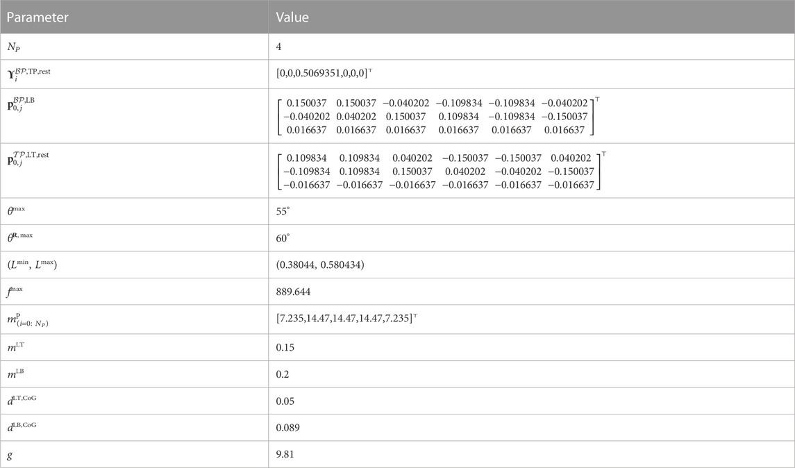
Experimental Results Parameters.

For even i, The values of ${\mathbf{p}}_{i,j}^{\mathcal{B}\mathcal{P},\text{LB}}$ and ${\mathbf{p}}_{i,j}^{\mathcal{T}\mathcal{P},\text{LT},\text{rest}}$ are equal to ${\mathbf{p}}_{0,j}^{\mathcal{B}\mathcal{P},\text{LB}}$ and ${\mathbf{p}}_{0,j}^{\mathcal{T}\mathcal{P},\text{LT},\text{rest}}$, respectively. For odd i, we have

$\begin{array}{cc}\hfill {\mathbf{p}}_{i,j}^{\mathcal{B}\mathcal{P},\text{LB}}& =R^{\text{odd}}{\mathbf{p}}_{0,j}^{\mathcal{B}\mathcal{P},\text{LB}}\hfill \\ \hfill {\mathbf{p}}_{i,j}^{\mathcal{T}\mathcal{P},\text{LT},\text{rest}}& =R^{\text{odd}}{\mathbf{p}}_{0,j}^{\mathcal{T}\mathcal{P},\text{LT},\text{rest}}\hfill \end{array}(28)$

Where R^odd is a 30-degree rotation about the z-axis,

$R^{\text{odd}}=\left[\begin{array}{ccc}\hfill \frac{\sqrt{3}}{2}\hfill & \hfill -\frac{1}{2}\hfill & \hfill 0\hfill \\ \hfill \frac{1}{2}\hfill & \hfill \frac{\sqrt{3}}{2}\hfill & \hfill 0\hfill \\ \hfill 0\hfill & \hfill 0\hfill & \hfill 1\hfill \end{array}\right](29)$

5.1 Pose generation

We describe the procedure for generating the dataset of poses that we use to generate end-effector goal positions for the computational studies in this work. This generation begins with the generation of individual random poses for the intended SP configuration. Given that the target 4-SP Assembler consists of four separate robots, poses can be generated by applying kinematic operations on each constituent SP separately, then stacking them, resulting in a full pose for the Assembler.

Pose generation for the individual SPs came in two varieties: Uniform and Extreme. Uniform poses were generated by applying the FK algorithm to a SP with a set of leg lengths uniformly generated from their minimum and maximum extensions. Configurations that resulted in an error or were at the “home” position (via error correction) were discounted, and iteration continued until a set number of poses (for the purpose of this paper, 10,000) were generated. Extreme poses followed the same procedure, with the added caveat that poses which did not meet a minimum measure of rotation magnitude of 30-degrees were also rejected, leaving only poses with the requisite tilt factor. Tilt was selected as being more important than translation because a tilt in one platform has a much greater change potential in a stack end effector than does translation.

Once individual SP poses were completed, the 4-SP stacked poses could be constructed. There were three categories of poses which we trialed: Uniform, Extreme, and Repeated. Uniform poses drew from the aforementioned uniform individual poses, while Extreme drew from the extreme poses. For both, four poses are chosen at random from their constituent files and applied to create a stacked pose. The end effector position (topmost plate of the topmost SP) is recorded, along with the plate positions and leg lengths of all constituent platforms. The Repeated poses differ slightly in generation. They too draw from the extreme pose file, but only one individual SP pose is chosen, and is applied to each platform in the stack, such that the ultimate pose is severely biased towards tilt in the direction of the constituent SP pose. For the purposes of this analysis, each type of pose generator produced three files consisting of 100, 1,000, and 10,000 poses respectively. The 100 pose file is intended purely for testing, whereas the two larger datasets for each type were earmarked for analysis.

5.2 Pose optimization

In this section, we compare the SIK and OPT methods for solving the IK problem on the instances generated in Section 5.1. We also include the force-related information for the initially generated poses (GEN) as a reference.

Table 1 summarizes the performance of the SIK and OPT methods on various instances, while Table 2 summarizes some additional performance characteristics determined during meta-analysis. A pose is said to be valid the end effector and base plates are in the correct pose, and all constraints related to kinematic validity are satisfied. A valid pose is said to be force-valid if the maximum-force constraints are also satisfied. The Avg % and Avg Max % Reduced metrics measure the percent reduction of forces out of the instances for which both methods yield kinematically valid poses. The % Improved metric measures the percentage of poses for which OPT yielded a better pose then SIK, out of the poses for which at least one of the methods yielded a valid pose. Finally, the Avg OPT Time metric measures the average time required for the OPT method to terminate, regardless of termination status.

TABLE 1

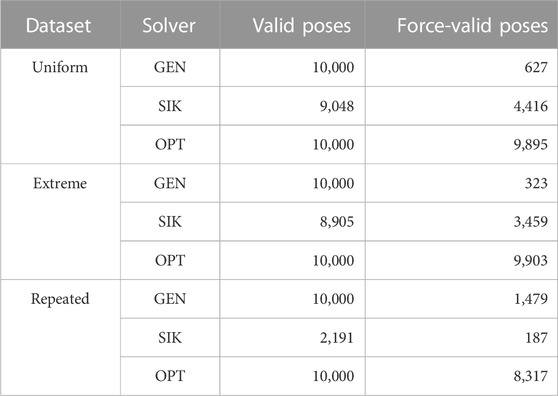
TABLE 1. Performance metrics for SIK and OPT, out of 10,000 random poses.

TABLE 2

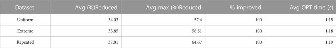
TABLE 2. Improvement of OPT over SIK, along with average computational time for 10,000 random poses.

Note that the optimizer is always able to find kinematically valid poses when initialized via the same-SP approach, even when the initial guesses are not kinematically valid. This effectiveness is especially noticeable for poses from the difficult Repeated datasets, for the success rate from SIK was only about 22%.

Figure 7 showcases the force-performance for the SIK and OPT approaches. From the figure, note that, particularly for the repeated dataset, the problems yielding kinematically valid poses for SIK are significantly less likely to yield force-invalid poses in OPT.

FIGURE 7

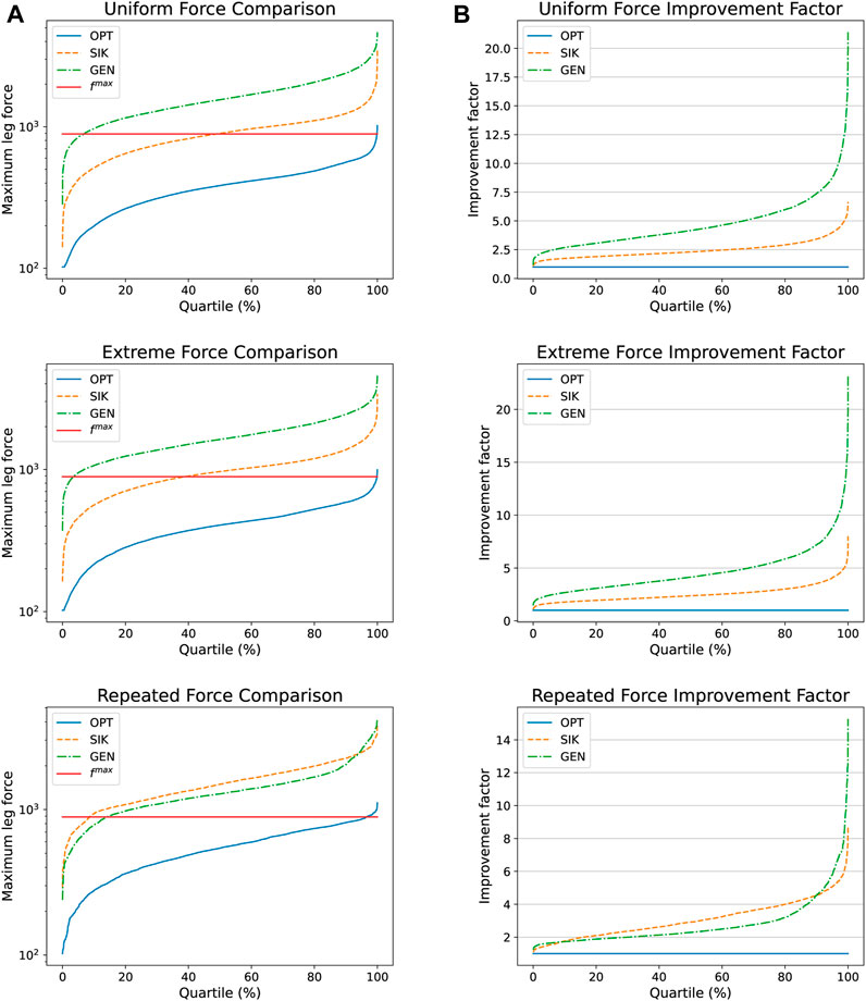
FIGURE 7. Pose comparison of OPT, GENerated, and SIK forces, considering the poses for which both approaches yielded kinematically valid poses. (A) Comparison of maximum leg forces, (B) Factor of improvement of OPT over each method. Forces are in Newtons. The mass of the actuators and Assembler plates as well as a 5 kg mass at the final End Effector are taken to account in the experiments.

Figure 8 showcases the computational performance of the optimizer over the Extreme and Repeated instances. The Uniform performance plot is omitted due to its strong similarity to the Extreme plot, but with one outlier requiring more than 16s. Note that the time-performance for the Repeated poses is more polarized than for other datasets: ∼55% (vs. ∼40%) of poses solve in less than 1s, but ∼10% (vs. ∼3%) require more than 2s to solve.

FIGURE 8

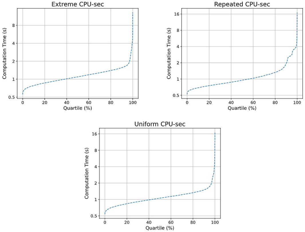
FIGURE 8. Computation times for OPT over 10,000 poses for the Extreme and Repeated instance families.

From Table 1 and Figure 7, we see a very strong degree of improvement in the resulting forces compared to the SIK heuristic. The forces are at least halved between 70% and 80% of the time, with improvement factors over 8 in some cases. This improvement, combined with the fast computation times observed in Figure 8, renders the OPT approach a viable method for the generation of force-optimized poses for SPs. Note that, in terms of forces, even the SIK approach was typically able to find much better poses than were initially generated, when it succeeded in generating a kinematically valid pose.

5.3 Trajectory planning

In this section, we demonstrate the effectiveness of the trust region method, then showcase how this method can be used in conjunction with RRT* to obtain good obstacle-avoiding paths very quickly after pre-processing.

To demonstrate the effectiveness of the trust region method, we showcase a difficult motion: a transition between opposite bent-over poses. We showcase using the thin-plated SP with ɛ^pos = 0.2, ${\epsilon }^{\text{rot}}=\frac{\pi }{3}$, λ^force = 0.04, λ^pose = 0.96, and λ^avg = 0.05. The sample motion, along with a plot showing the progression of the motion in terms of the forces and the maximum plate global-frame distances from any plate to the ending pose, is shown in Figure 9.

FIGURE 9

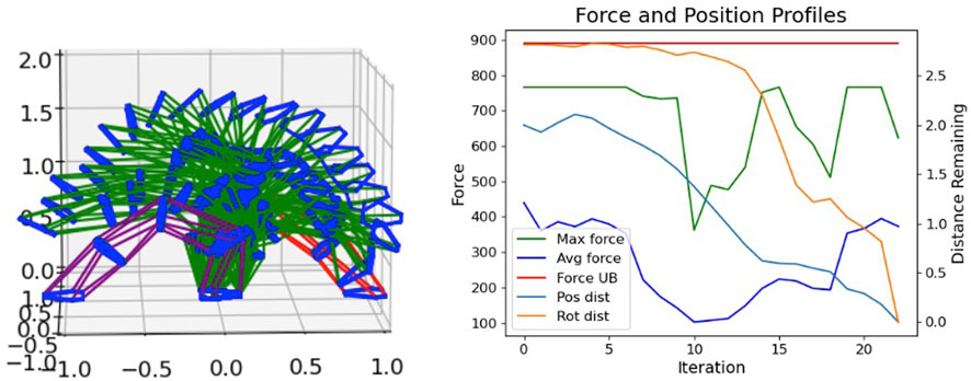
FIGURE 9. Force-controlled transition between bent-over poses using trust region method. (Left) Axes units are in meters. (Right) Force in Newtons. The mass of the actuators and Assembler plates as well as a 5 kg mass at the final End Effector are taken to account in the experiments.

To demonstrate the consistency and performance of the trust region method, we compare the trust region method with the direct transformation and the RRT* approach.

A comparison trajectory planning results for all datasets are shown in Table 3. The settings used for the trust-region method were ɛ^pos = 0.1, ${\epsilon }^{\text{rot}}=\frac{\pi }{6}$, λ^force = 0.04, λ^pose = 0.96, and λ^avg = 0.05. Some primary metrics of the solution are given as

1. Behaved: A path is considered behaved if the maximum leg forces mid-motion do not exceed the maximum forces at the starting or ending pose.

2. Force-Valid: A path is considered force-valid if either all leg forces are valid throughout the motion, or if the path is behaved with excessive leg forces at either the starting or ending pose.

3. Avg OPT Time: The average optimization time across all tests.

TABLE 3

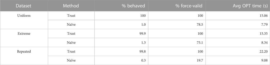
TABLE 3. Comparison of trajectory planning results for trust-region vs. naïve FK, out of 1,000 random poses.

We show a more complete picture of the maximum leg forces resulting from the two approaches in Figure 10, and compare the motion energies in Figure 11. To estimate the motion energies, we assume that extending a leg under tensile forces and contracting a leg under compression forces are free operations, and count only the portions of the motions that require energy input.

FIGURE 10

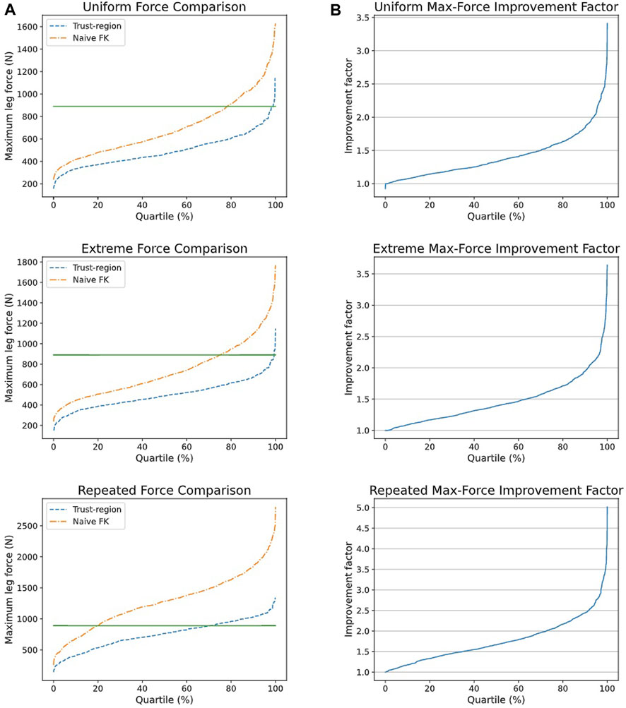
FIGURE 10. Comparison of maximum forces between trajectory planning methods. (A) Comparison of maximum forces, (B) Factor of improvement of trust-region method over naïve interpolated FK. The green line represents the maximum allowed force.

FIGURE 11

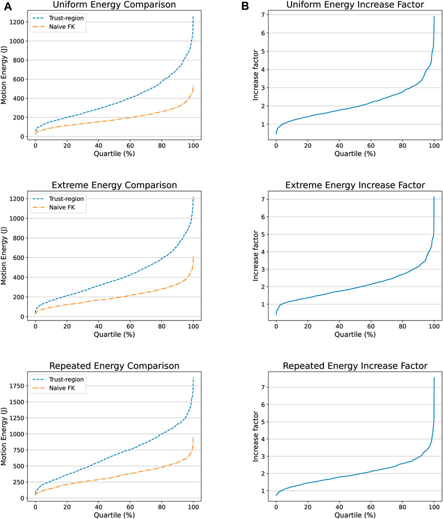
FIGURE 11. Comparison of motion energies between trajectory planning methods. (A) Comparison of motion energies, (B) Extra-energy factor of trust-region method over naïve interpolated FK.

The results reveal that the trust region method is far more consistent, with maximum forces only rarely exceeding those at the end effectors (in 0.1% of cases), and with maximum-force improvements as high as a factor of 5. However, the gains in maximum forces and consistency come at a price: the motion energies tend to be far higher, exceeding the more direct motions by as much as a factor of 7. Furthermore, the naïve approach solves roughly twice as quickly as the trust region approach. Thus, in practice, we recommend first computing the naïve motion, then applying the trust region method if the motion is either near-infeasible or very poorly behaved, with mid-motion max-forces far higher then endpoint max-forces.

Note that, in practice, any leg motion requires some baseline motor energy usage even under zero net forces, which would further strengthen the energy advantage gained from the shorter naïve motions.

5.4 Range of motion analysis

Using a stochastic method, we analyzed the range of motion for the SIK method for both the thin and thick-plated SPs. The results are shown in Figure 12.

FIGURE 12

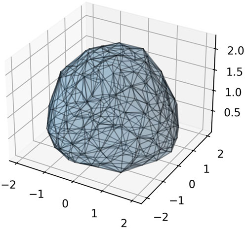
FIGURE 12. Range of motion approximation for the test Assembler used in our computational experiments. Axes units are in meters. Plot shows points where the end-effector can be located. Note that there is a hole in the middle of this image since certain shorter end-effector points are not reachable.

For a single SP, the simplified range of motion (ROM) methodology is to create a number of concentric scaled unit spheres centered at the platform’s rest pose (a sphere with a certain number of points evenly distributed about its exterior surface) and calculate IK for each point, along with perturbing the rotations at the extremes. Points that succeed are admitted into the ROM cloud, and those that do not are discarded. The final ROM graphic is created by utilizing the technique Alpha-Shapes in order to create a concave hull illustrating the reachability of the platform.

6 Conclusion

We have presented a fast approach for the force-optimization of stacked SPs that can significantly improve their range of motion under heavy loads. In particular, the optimization step can result in reductions of the worst-case leg forces by as much as an order of magnitude in some cases. Further, we have presented a fast, consistent trust-region trajectory planning approaches based on this pose optimization scheme, and demonstrated the effectiveness of the approach in comparison to a simple length-based optimization approach.

In the future, the ultimate goal is to use these stacked SP structures to perform automated assembly operations. To improve on the pose optimization approach, we suggest exploring the use of more robust heuristics in conjunction with the local optimizer proposed in this work. For example, to improve pose optimization given fixed base and end-effector positions, one could quickly compute rough bounds on the possible poses for the middle plates, then apply heuristics such as a genetic algorithm or a bidirectional search, with frequent or intermittent local optimization steps, to quickly hone in on a solution. Alternatively, one could construct some fast heuristic for generating randomized feasible or near-feasible poses for a fixed end-effector position, then locally optimize a moderate number of random poses in parallel to seek a stronger solution with limited additional computational cost.

Lastly, it may be possible to make our objective function for the trajectory optimization more realistic. Our objective tracks the amount of energy used over time. However, since the amperage needed for expansion and contraction of the leg joints is a nonlinear function of the movement, we may be able to study this function using our hardware to model a better objective function that reflects the amperage used for each movement. This will require further hardware experimentation.

Data availability statement

The raw data supporting the conclusion of this article will be made available by the authors, without undue reservation.

Author contributions

BB is responsible for the force-based inverse kinematics optimization math, pose optimization, and trust-based trajectory planning. WC is responsible for determining the kinematic constraints for the Stewart platform chain, force calculations, pose generation, and trajectory planning. SC created a hardware load-cell equipped Stewart platform to test the force feedback and use data to verify the mathematical model. RH and EK are advisors for this project and provided ideas and guidance on approaches in addition to writing and editing the manuscript. All authors contributed to the article and approved the submitted version.

Funding

Some of this material is based on work supported by NASA via contract 80LARC20P0020 for the “Assemblers: A modular and reconfigurable manipulation system for autonomous in-space assembly” project. Additionally, this material was also partially based on work sponsored by the Northrop Grumman Undergraduate Research Experience in Industrial & Systems Engineering at Virginia Tech project. Any opinions, findings, and conclusion or recommendations expressed in this material are those of the authors and do not necessarily reflect the views of the Northrop Grumman Corporation. RH and BB are funded by AFOSR grant FA9550-21-0107.

Conflict of interest

The authors declare that the research was conducted in the absence of any commercial or financial relationships that could be construed as a potential conflict of interest.

Publisher’s note

All claims expressed in this article are solely those of the authors and do not necessarily represent those of their affiliated organizations, or those of the publisher, the editors and the reviewers. Any product that may be evaluated in this article, or claim that may be made by its manufacturer, is not guaranteed or endorsed by the publisher.

Author disclaimer

Any opinions, findings, and conclusion or recommendations expressed in this material are those of the authors and do not necessarily reflect the views of the Air Force Office of Scientific Research.

Supplementary material

The Supplementary Material for this article can be found online at: https://www.frontiersin.org/articles/10.3389/fmech.2023.1225828/full#supplementary-material

References

Balaban, D., Cooper, J., and Komendera, E. (2019). “Inverse kinematics and sensitivity minimization of an n-stack Stewart platform,” in 2019 IEEE/RSJ international conference on intelligent robots and systems (IROS) (IEEE), 6794–6799.

CrossRef Full Text | Google Scholar

Bangjun, L., Likun, P., and Tingtao, M. (2012). “Improving dynamic performance of Stewart platforms through optimal design based on evolutionary multi-objective optimization algorithms,” in Proceedings of the 1st international conference on mechanical engineering and material science (Atlantis Press), 294–298.

CrossRef Full Text | Google Scholar

Bingul, Z., and Karah, O. (2012). “Dynamic modeling and simulation of Stewart platform,” in Serial and parallel robot manipulators - kinematics, dynamics, control and optimization (InTech), 19–42.

CrossRef Full Text | Google Scholar

Bynum, M. L., Hackebeil, G. A., Hart, W. E., Laird, C. D., Nicholson, B. L., Siirola, J. D., et al. (2021). Pyomo–optimization modeling in python. 67third edition. Springer Science & Business Media.

Google Scholar

Charters, T., Enguica, R., and Freitas, P. (2009). Detecting singularities of Stewart platforms. Mathematics-in-Industry Case Stud. J. 1, 66–80.

Google Scholar

Chen, H., Chen, W., and Liu, J. (2007). Optimal design of Stewart platform safety mechanism. Chin. J. Aeronautics 20 (4), 370–377. doi:10.1016/s1000-9361(07)60057-0

CrossRef Full Text | Google Scholar

Cooper, J. R., Neilan, J. H., Mahlin, M., and WhiteAssemblers, L. M (2022). A modular, reconfigurable manipulator for autonomous in-space assembly.

Google Scholar

Cortes, J., and Simeon, T. (2003). 2003 IEEE international conference on robotics and automation (cat. No.03CH37422). IEEE, 4354–4359.Probabilistic motion planning for parallel mechanisms

Google Scholar

Dorsey, J., Sutter, T., and Wu, K. (1992). Structurally adaptive space crane concept for assembling space systems on orbit. NASA Langley Research Center. Technical report.

Google Scholar

Dragan, A., and Srinivasa, S. (2014). Integrating human observer inferences into robot motion planning. Auton. Robots 37 (4), 351–368. doi:10.1007/s10514-014-9408-x

CrossRef Full Text | Google Scholar

Ernandis, R. (2021). PhD thesis. College Park: University of Maryland.Sampling based motion planning for minimizing position uncertainty with Stewart platforms

Google Scholar

Grosch, P., Gregorio, R. D., Lopez, J., and Thomas, F. (2010). “Motion planning for a novel reconfigurable parallel manipulator with lockable revolute joints,” in 2010 IEEE international conference on robotics and automation (IEEE), 4697–4702.

CrossRef Full Text | Google Scholar

Hart, W. E., Watson, J.-P., and Woodruff, D. L. (2011). Pyomo: modeling and solving mathematical programs in python. Math. Program. Comput. 3 (3), 219–260. doi:10.1007/s12532-011-0026-8

CrossRef Full Text | Google Scholar

Ichnowski, J., Avigal, Y., Satish, V., and Goldberg, K. (2020). Deep learning can accelerate grasp-optimized motion planning. Sci. Robot. 5 (48), eabd7710. doi:10.1126/scirobotics.abd7710

PubMed Abstract | CrossRef Full Text | Google Scholar

Islam, F., Nasir, J., Malik, U., Ayaz, Y., and Hasan, O. (2012). RRT*-Smart: rapid convergence implementation of RRT* towards optimal solution. IEEE.

Google Scholar

Karaman, S., and Frazzoli, E. (2011). Sampling-based algorithms for optimal motion planning. Int. J. Rob. Res. 30 (7), 846–894. doi:10.1177/0278364911406761

CrossRef Full Text | Google Scholar

Kuffner, J., and LaValle, S. (2000). RRT-connect: an efficient approach to single-query path planning. In Proceedings 2000 ICRA. Millennium conference. IEEE international conference on robotics and automation. Symposia proceedings (cat. No.00CH37065). IEEE, 2, 995–1001.

Google Scholar

LaValle, S. M. (1998). Rapidly-exploring random trees: a new tool for path planning. The annual research report.

Google Scholar

Lazard, D., and Merlet, J.-P. (1994). The (true) Stewart platform has 12 configurations, 2160–2165.

Google Scholar

Lei, Z., and Xiaolin, D. (2013). “Optimize the redundant 6-DOF Stewart platform based on ant colony optimization,” in Proceedings of 2013 3rd international conference on computer science and network technology (IEEE), 1238–1241.

CrossRef Full Text | Google Scholar

Li, Y.-W., Wang, J.-S., and Wang, L.-P. (2002). Stiffness analysis of a Stewart platform-based parallel kinematic machine. Proc. 2002 IEEE Int. Conf. Robotics Automation (Cat. No.02CH37292) 4, 3672–3677.

Google Scholar

Lynch, K. M., and Park, F. C. (2017). Modern robotics: mechanics, planning, and control. Cambridge, UK: Cambridge University Press. OCLC: ocn983881868.

Google Scholar

Majid, M. Z. A., Huang, Z., and Yao, Y. L. (2000). Workspace analysis of a six-degrees of freedom, three-prismatic- prismatic-spheric-revolute parallel manipulator. Int. J. Adv. Manuf. Technol. 16 (6), 441–449. doi:10.1007/s001700050176

CrossRef Full Text | Google Scholar

Merlet, J. P. (2006). Parallel robots. Springer.

Google Scholar

Miura, K., and Furuya, H. (1988). Adaptive structure concept for future space applications. AIAA J. 26 (8), 995–1002. doi:10.2514/3.10002

CrossRef Full Text | Google Scholar

Moser, J., and Cooper, J. (2019). A reinforcement learning approach for the autonomous assembly of in-space habitats and infrastructures in uncertain environments. 22nd IAA Symposium on Human Exploration of the Solar System. International Astronautical Conference.

Google Scholar

Nguyen, C., Antrazi, S., Zhou, Z.-L., and Campbell, C. (1991). “Experimental study of motion control and trajectory planning for a Stewart Platform robot manipulator,” in Proceedings. 1991 IEEE international conference on robotics and automation (IEEE Comput. Soc. Press), 2, 1873–1878.

Google Scholar

Nguyen, C. C., and Antrazi, S. (1990). Trajectory planning and control of a 6 dof manipulator with Stewart platform-based mechanism. NASA Goddard Space Flight Center. Technical report.

Google Scholar

Osa, T., Esfahani, A. M. G., Stolkin, R., Lioutikov, R., Peters, J., and Neumann, G. (2017). Guiding trajectory optimization by demonstrated distributions. IEEE Robot. Autom. Lett. 2 (2), 819–826. doi:10.1109/lra.2017.2653850

CrossRef Full Text | Google Scholar

Quintero-Pena, C., Kyrillidis, A., and Kavraki, L. E. (2021). Robust optimization-based motion planning for high-DOF robots under sensing uncertainty. IEEE.

Google Scholar

Ríos, A., Hernández, E. E., and Valdez, S. I. (2021). A two-stage mono- and multi-objective method for the optimization of general UPS parallel manipulators. Mathematics 9 (5), 543. doi:10.3390/math9050543

CrossRef Full Text | Google Scholar

Santos, J. C., and da Silva, M. M. (2017). Investigation of motion planning methods with a kinematically redundant manipulator.

Google Scholar

Schulman, J., Duan, Y., Ho, J., Lee, A., Awwal, I., Bradlow, H., et al. (2014). Motion planning with sequential convex optimization and convex collision checking. Int. J. Robotics Res. 33 (9), 1251–1270. doi:10.1177/0278364914528132

CrossRef Full Text | Google Scholar

Sun, T., and Lian, B. (2018). Stiffness and mass optimization of parallel kinematic machine. Mech. Mach. Theory 120, 73–88. doi:10.1016/j.mechmachtheory.2017.09.014

CrossRef Full Text | Google Scholar

Szynkiewicz, W., and Błaszczyk, J. (2011). Optimization-based approach to path planning for closed chain robot systems. , 21(4):659–670. doi:10.2478/v10006-011-0052-8

CrossRef Full Text | Google Scholar

Toz, M., and Kucuk, S. (2013). Dexterous workspace optimization of an asymmetric six-degree of freedom Stewart–Gough platform type manipulator. Robotics Aut. Syst. 61 (12), 1516–1528. doi:10.1016/j.robot.2013.07.004

CrossRef Full Text | Google Scholar

Virtanen, P., Gommers, R., Oliphant, T. E., Haberland, M., Reddy, T., Cournapeau, D., et al. (2020). SciPy 1.0: fundamental algorithms for scientific computing in Python. Nat. Methods 17, 261–272. doi:10.1038/s41592-019-0686-2

PubMed Abstract | CrossRef Full Text | Google Scholar

Volz, A., and Graichen, K. (2018). An optimization-based approach to dual-arm motion planning with closed kinematics. IEEE.

Google Scholar

Wächter, A., and Biegler, L. T. (2005). On the implementation of an interior-point filter line-search algorithm for large-scale nonlinear programming. Math. Program. 106 (1), 25–57. doi:10.1007/s10107-004-0559-y

CrossRef Full Text | Google Scholar

Wang, P., Yang, H., and Xue, K. (2015). Jerk-optimal trajectory planning for Stewart platform in joint space. In 2015 IEEE international conference on mechatronics and automation (ICMA), 1932–1937. IEEE.

CrossRef Full Text | Google Scholar

Williams, R. L. (1995). “Survey of active truss modules,” in Volume 1: 21st design automation conference (American Society of Mechanical Engineers).

CrossRef Full Text | Google Scholar

Xie, Z., Li, G., Liu, G., and Zhao, J. (2017). Optimal design of a Stewart platform using the global transmission index under determinate constraint of workspace. Adv. Mech. Eng. 9 (10), 168781401772088. doi:10.1177/1687814017720880

CrossRef Full Text | Google Scholar

Yokoi, K., Komoriya, K., and Tanie, K. (1992). A method for solving inverse kinematics of variable structure truss arm with high redundancy. J. Intelligent Material Syst. Struct. 3 (4), 631–645. doi:10.1177/1045389x9200300406

CrossRef Full Text | Google Scholar

Zhang, B. (2005). Design and implementation of A 6 dof parallel manipulator with passive force control. PhD thesis, University of Florida.

Google Scholar

Zucker, M., Ratliff, N., Dragan, A., Pivtoraiko, M., Klingensmith, M., Dellin, C., et al. (2013). Chomp: covariant Hamiltonian optimization for motion planning. Int. J. Robotics Res. 32 (9), 1164–1193. doi:10.1177/0278364913488805

CrossRef Full Text | Google Scholar