Identifying a machine-learning structural descriptor linked to the creep behavior of Kob-Andersen glasses

A wide variety of materials, ranging from metals to concrete, experience, typically at high-temperatures or over long time scales, permanent deformations when subjected to sustained loads below their yield stress—a phenomenon known as creep. While theories grounded on defects such as vacancies, dislocations, or grain boundaries can explain creep in crystalline materials, our understanding of creep in disordered solids remains incomplete due to the lack of analogous structural descriptors. In this study, we use molecular dynamics to simulate the creep response of a Kob-Andersen glass model system under constant, uniaxial, compressive stress at finite temperature. We leverage that data to derive, using a machine-learning classification model, a structural descriptor termed looseness, $\mathbb{L}$, which is based on simple and interpretable local structural features and can predict imminent plastic rearrangements within the glass. We show that the average looseness of the system evolves logarithmically with time, mirroring the time dependence of the creep strain and demonstrating the ability of our model to bridge local, short-term particle dynamics with the long-term macroscopic creep response. A detailed feature importance analysis reveals the particular significance of short-range structural heterogeneity in the prediction. We also scrutinize the spatial and temporal correlations of looseness, which mirror the lack of long-range order in glasses and their dynamic heterogeneity. Our research underscores the substantial predictive potential of machine-learning-derived structural indicators in systems experiencing concurrent stress and thermal excitations, paving the way for future work to elucidate the interplay between thermal and mechanical activation of structural defects in disordered solids.

1 Introduction

Certain materials, when exposed to sustained loads below their yielding point, and typically over long time scales and/or high temperatures, exhibit permanent deformations—a phenomenon known as creep. Creep occurs in metals under high-temperature conditions, such as those found in turbine blades (McLean, 1966), in ice causing glaciers to flow (Weertman, 1983), or in amorphous materials such as polymers (Brinson and Gates, 1995), metallic glasses (Castellero et al., 2008), or even concrete (Bazant and Wittmann, 1982), the most used man-made material worldwide. While several mechanisms responsible for creep of crystalline solids have been proposed, which include the diffusion of vacancies (Nabarro, 1948; Herring, 2004), dislocation dynamics (Harper and Dorn, 1957), or grain boundary sliding (Bell and Langdon, 1967; Langdon, 2006), all these mechanisms are based on structural defects that break the long-range order of the crystal lattice and therefore can be trivially identified. Analogous knowledge for disordered solids is understandably lacking, as what constitutes as a structural defect in these systems remains an open question. For example, intuitive structural descriptors, such as free volume or bond orientational order, have been shown to be poor predictors of the plasticity of glasses (Richard et al., 2020). Other more successful indicators have also been proposed such as soft-modes (Widmer-Cooper et al., 2008; Tanguy et al., 2010), or rattling amplitude (Larini et al., 2008), but those rely on the dynamics of the system and thus are not strictly structural.

Motivated by this challenge and the tremendous power of machine learning (ML) techniques to find patterns within complex datasets, when human intuition falls short (Bishop and Nasrabadi, 2006), (Cubuk et al., 2015) pioneered the use of ML techniques to identify potentially complex structural signatures that are predictive of the particle dynamics in glassy systems. In this context and given the challenge of collecting experimental data at the needed time and length scales, molecular dynamics (MD) simulations have become indispensable in generating high-quality, comprehensive data sets essential for the successful implementation of ML models. Despite the remarkable advancements made in this field over the past few years (Schoenholz et al., 2016; Wang and Jain, 2019; Bapst et al., 2020; Boattini et al., 2020; Fan et al., 2020; Wang et al., 2020; Liu et al., 2021; Peng et al., 2021; Wang and Zhang, 2021; Xiao et al., 2021; Wu et al., 2023), prior studies have tackled thermally-driven and stress-driven relaxation events independently. Studies focused on understanding structural signatures underlying the glass transition are based on simulations of stress-free glasses near the glass transition temperature. In contrast, those focused on predicting plastic rearrangements in disordered solids under stress rely, almost exclusively, on simulations of the glass under athermal, quasistatic shear conditions. Moreover, to the best of our knowledge, the recent work by Liu et al. (2021) stands alone in its focus on creep. Interestingly, they demonstrated, for shear strains up to approximately 1%, a strong correlation between the macroscopic creep rate and a structural descriptor derived through ML based on the initial undeformed structure of the disordered colloidal gel (Liu et al., 2021). Their simulations, however, were conducted in the quasistatic athermal regime and under oscillatory shear, which is a condition more closely related to fatigue behavior than to creep. Deriving ML structural descriptors that can predict the creep response of disordered solids under sustained loads at finite temperatures remains a largely unexplored area, and it is extremely relevant in the context, for example, of bulk metallic glasses operating at high temperatures (Li et al., 2019).

Here, we employ MD simulations to investigate the creep response of a Kob-Andersen (KA) glass (Kob and Andersen, 1995) under sustained uniaxial compressive stress at finite temperature. We provide a detailed analysis of how the macroscopic creep response of the glass is affected by the level of applied stress and temperature, as well as characterize the statistical evolution during creep of the microscopic deformations, which we characterize by the non-affine squared displacements of individual particles in the glass, $D_{\min }^2$. Using ML classification methods based on interpretable structural features describing the particles interstices, we are able to identify a local structural descriptor, dubbed looseness, $\mathbb{L}$, that can predict whether a particle in the glass will undergo an imminent plastic rearrangement based on its local interstitial environment alone. We quantify the prediction accuracy of the ML models, and explain it based on the interstitial structural features. We also study the time evolution of looseness averaged over all the particles in the glass, $〈\mathbb{L}〉$, as well as its spatial and temporal correlations.

2 Materials and methods

2.1 Molecular dynamics simulations

We performed MD simulations using the program LAMMPS (Thompson et al., 2022) to study the creep response of a KA glass under a sustained compressive stress at finite temperature. The KA model is a two-component Lennard-Jones (LJ) system, which has been extensively used to study the dynamics of supercooled liquids and the glass transition, due to being relatively simple and computationally efficient while still being able to capture many of the key behaviors of real glasses (Kob and Andersen, 1995). All the simulated systems here contained 10,000 particles, where 80% and 20% of them were type A and type B, respectively. The parameters of the LJ interactions are: ${\mathrm{\sigma }}_{\mathrm{A}\mathrm{A}}=1.0$, ${\mathrm{\sigma }}_{\mathrm{A}\mathrm{B}}=0.8$, ${\mathrm{\sigma }}_{\mathrm{B}\mathrm{B}}=0.88$, ${ϵ}_{\mathrm{A}\mathrm{A}}=1.0$, ${ϵ}_{\mathrm{A}\mathrm{B}}=1.5$, ${ϵ}_{\mathrm{B}\mathrm{B}}=0.5$, ${\mathrm{m}}_{\mathrm{A}}={\mathrm{m}}_{\mathrm{B}}=1$, and the cutoff for the interactions was set to $2.5{\mathrm{\sigma }}_{\mathrm{A}\mathrm{A}}$. All the quantities reported in this study are given in reduced Lennard-Jones units, unless specified otherwise. All the simulations were performed with periodic boundary conditions (PBCs) in all dimensions (effectively simulating bulk glasses), and a time step $\mathrm{\tau }=0.01$.

We generated initial glass configurations as follows. First, we generated a random configuration of particles in a simulation box at density $\rho =N/V=1.2$, which is the equilibrium density of the KA glass. We simulated this system in the NVT ensemble for $5\times {10}^4$ steps, using a Langevin thermostat at $\mathrm{T}=3$, which is well above the mode-coupling temperature of the KA model, ${\mathrm{T}}_{\mathrm{M}\mathrm{C}\mathrm{T}}=0.435$ (Ashwin and Sastry, 2003). Once having randomized the positions of the particles, we induced glass formation by cooling down the system to $\mathrm{T}=0.1$ over ${10}^4$ steps in the NVT ensemble using a Nose-Hoover thermostat. As a final step, we minimized the energy of the system. We generated a total of ten unique, minimized, initial glass configurations following this process.

Starting from each of those ten glass configurations, we performed simulations in the NPT ensemble where the KA glasses were instantaneously placed under a constant uniaxial compressive stress at $T$ below ${\mathrm{T}}_{\mathrm{M}\mathrm{C}\mathrm{T}}$ and sustained for ${10}^7$ steps. During the simulations, we outputted optimized configurations, where the energy of the system was minimized under the constraint of the applied stress, every ${10}^4$ steps for analysis. From each MD simulation, we therefore collect ${10}^3$ optimized configurations for analysis. We carried out simulations at $\mathrm{T}=0.01$, $0.1$, $0.2$, $0.3$, and $0.4$ at a stress of ${\mathrm{\sigma }}_0=0.5$, and simulations at stress levels ranging from ${\mathrm{\sigma }}_0=0.1$ to $0.9$ in increments of 0.1, at a temperature of $\mathrm{T}=0.1$. We also performed ten simulations at ${\mathrm{\sigma }}_0=0.5$ and $\mathrm{T}=0.1$. The data from these simulations (${\mathrm{\sigma }}_0=0.5$ and $\mathrm{T}=0.1$), which demonstrably reproduce the primary creep response of the KA glass, were utilized for the ML tasks.

2.2 Analysis of non-affine displacements

We calculated the non-affine squared displacement of particle $i$ over a time interval $\Delta t$ measured from $t_o$, $D_{\min }^2\left(i,t_o,∆t\right)$, using the equations originally proposed by Langer and Falk (Falk and Langer, 1998), which can be written as:

$D_{\min }^2\left(i,t_o,∆t\right)=\underset{{\mathrm{\epsilon }}_i}{\min }\left\{\frac{1}{n_i}{\displaystyle \sum _j}{\left[R_{ij}\left(t_o+∆t\right)-{\mathrm{\epsilon }}_i{R}_{ij}\left(t_o\right)\right]}^2\right\}(1)$

where ${\mathrm{\epsilon }}_i$ is the local strain tensor around particle $i$ which minimizes the quantity between the curly brackets, $n_i$ is the number of particles within a cutoff distance ($R_{\mathrm{c}\mathrm{u}\mathrm{t}}$) of particle $i$, and $R_{ij}$ is the distance between particle $i$ and particle $j$ in its neighborhood. We select $R_{\mathrm{c}\mathrm{u}\mathrm{t}}=2.5$, beyond which the results for $D_{\min }^2$ showed no sensitivity to variations in this parameter. The quantity ${\mathrm{\epsilon }}_i{R}_{ij}\left(t_o\right)$ corresponds to the inter-particle distances predicted at $t_o+∆t$ after the affine deformation. We used our own MATLAB script to compute $D_{\min }^2$.

2.3 Machine learning

2.3.1 Problem statement

Our ultimate goal is to train a ML model that can predict whether or not a particle will undergo a plastic rearrangement ($D_{\min }^2>D_{\min ,0}^2$) over some time interval $∆t$, using as features only simple structural descriptors of the local neighborhood of that particle. Accordingly, we cast this problem as a supervised binary classification task. We call particles that undergo plastic rearrangements class 1 or loose, and those that do not class 0 or tight.

2.3.2 Dataset

Each particle in each of the configurations outputted during the MD simulations at $t_o={1\times 10}^4,{2\times 10}^4,\dots ,{10}^3{\times 10}^4$ steps, corresponds to an example in the dataset. The features for each particle are calculated at each $t_o$ and the particles are labeled as loose (class 1) or tight (class 0) depending on $∆t$ (the time interval over which the particle displacements are quantified) and $D_{\min ,0}^2$ (the threshold defining whether a particle undergoes substantial rearrangement). In this study, we focus only on the 80% of particles identified as type A, but our approach could be readily expanded to type B particles by choosing a different, suitable value for $D_{\min ,0}^2$. For $∆t={10}^4$ the dataset contains: $10$ independent MD simulations $\times$ ${10}^3$ configurations $\times$ $\mathrm{8,000}$ particles of type A ${=8\times 10}^7$ examples. As shown in Supplementary Table S1, our datasets are extremely imbalanced, with class 1, the loose particles, being the minority class as most particles in the glass do not undergo plastic rearrangements during creep.

2.3.3 Feature engineering

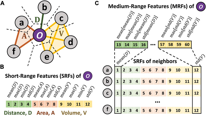
Inspired by the work by Wang and Jain (2019), we created features that encompass easily interpretable and straightforward structural quantities that capture the interstitial environments of each particle short- and medium-range length scales. The short-range features (SRFs) are derived from the free distances, areas, and volumes between a given particle and its neighbors. The distances, areas, and volumes, determined by pairs, triplets, and groups of four particles, respectively, are corrected for the spherical particle sizes (proportional to ${\mathrm{\sigma }}_{\mathrm{A}\mathrm{A}}$ and ${\mathrm{\sigma }}_{\mathrm{A}\mathrm{B}}$), therefore representing the interstitial non-occupied space. The nearest neighbors to any particle are found by identifying the particles associated with Voronoi cells that share a boundary with the cell of the particle in question. The tetrahedral volume is calculated using Quickhull algorithm (Barber et al., 1996). For each metric—distance, area, volume—we compute four features that correspond to the mean, maximum, minimum, and standard deviation of the calculated values for the given particle. Hence, there is a total of 12 SRFs (e.g., $\text{max}(\text{A},\dots$). The summary statistics aim to capture the average as well as potential anisotropy of the local interstitial environment. The medium-range features (MRFs) are computed by calculating the same summary statistics, but now of the SRFs corresponding to the neighbors of the given particle. Consequently, the MRFs consists of 48 features (e.g., $\mathrm{s}\mathrm{t}\mathrm{d}\left[\mathrm{m}\mathrm{e}\mathrm{a}\mathrm{n}\left(\mathrm{V}\right)\right]$, …). As illustrated in Figure 1, each particle is described by a total of 60 features.

FIGURE 1

FIGURE 1. Short-Range Features (SRFs) and Medium-Range Features (MRFs). (A) Particle O, surrounded by particles a, b, c, … , f which are neighbors according to a Voronoi construction depicted by black, dashed lines. A distance (green), an area (red), and a volume (yellow) element are illustrated in the sketch. (B) SRFs are calculated based on the summary statistics (mean, maximum, minimum, and standard deviation) of the distances, areas, and volumes defined by the particle O and its neighbors The numbers shown in the arrays correspond to the indexes of the corresponding features (1–12 are SRF, and 13 to 60 MRF). (C) The MRFs assigned to particle O comprise the summary statistics of the SRFs corresponding to the neighboring particles.

2.3.4 Workflow design

All the ML tasks in this paper were executed using Python scripts with the Scikit-Learn (Pedregosa et al., 2011) and Imbalanced-learn (Lemaître et al., 2017) packages. To evaluate and assess the ML models, we utilized balanced accuracy as our evaluation metric, which is the arithmetic mean of sensitivity, $TP/\left(TP+FN\right)$, and specificity, $TN/\left(TN+FP\right)$, where $T$ and $F$ stand for true and false, respectively, and $P$ and $N$ for positive and negative, respectively. This metric gives an equal weight to both classes, ensuring that neither the majority nor the minority class dominates the accuracy score. In this paper, we performed 3 ML tasks: 1) an investigation to select the optimal values for $∆t$ and $D_{\min ,0}^2$, 2) implementation of recursive feature elimination (RFE) to remove highly correlated features, reduce the model complexity, and gain insight into the most important features, and 3) training a ML classification model using the optimal values of $∆t$ and $D_{\min ,0}^2$, as well as the top ranked features.

To investigate the influence of $∆t$ and $D_{\min ,0}^2$ on the accuracy of the models, we first created, for each combination of $∆t={10}^4$, ${10}^5$, or ${10}^6$ steps and $D_{\min ,0}^2=0.05$, $0.1$, $0.15$, $0.20$, $0.25$, or $0.30$, five balanced bootstrap samples from the overall dataset using random undersampling. In random undersampling, instances of the majority class are randomly eliminated to equalize the number of instances in both the classes. Each of the five balanced samples contained 1,285 examples from each class. We maintained a consistent dataset size across all combinations of $∆t$ and $D_{\min ,0}^2$ to isolate the effect of these two parameters. For each of the balanced samples, we performed feature standardization to prevent domination by larger-scale features, thereby enabling all features to contribute evenly to model predictions. Next, we used cross-validation CV to identify the optimal regularization hyperparameter, $C$, for a logistic regression model. After determining the optimal $C$, we used 5-fold CV to compute the validation balanced accuracy of the models.

We used RFE, once established $∆t={10}^4$ and $D_{\min ,0}^2=0.25$, to remove highly correlated features, reduce the model complexity, and improve interpretability (McLean, 1966). Data from 8 of the 10 MD simulations were used for this task, with the remainder reserved for testing the final model. Using random undersampling, we generated five independent balanced bootstrap samples containing 2,115 instances from each class. After standardizing the features, RFE was then performed using a gradient boost classifier (GBC) as the estimator.

Using $∆t={10}^4$ and $D_{\min ,0}^2=0.25$ along with the top 10 ranked features identified through RFE, we trained an ML classification model to predict the particle labels. We applied the same training and testing split as in the RFE study and standardized the training and testing dataset features independently to avoid leakage. We used EasyEnsemble as our ML algorithm (Liu et al., 2009), where an ensemble of learners is trained on different balanced bootstrap samples. Random under-sampling was utilized to balance the samples. Our ensemble comprised 10 learners using logistic regression as the base estimator with an optimal regularization parameter $C=1$ (see Supplementary Table S2 for details). The model output, termed as looseness, $\mathbb{L}\in \left[\mathrm{0,1}\right]$, represents the probability of a particle being classified as loose or class 1. We decided to use logistic regression due to its simplicity and because it provides a probability for the predictions.

2.4 Fluctuations, space, and time autocorrelation functions

We calculated the space autocorrelation function of looseness, ${\mathrm{S}\mathrm{A}\mathrm{C}\mathrm{F}}_{\mathbb{L}}$, using:

${\mathrm{S}\mathrm{A}\mathrm{C}\mathrm{F}}_{\mathbb{L}}\left(\Delta r\right)={〈\left({\mathbb{L}}_i\left(t_0\right)-{〈\mathbb{L}\left(t_0\right)〉}_N\right)\bullet \left({\mathbb{L}}_j\left(\Delta r,t_0\right)-{〈\mathbb{L}\left(t_0\right)〉}_N\right)〉}_{ij,t_0}(2)$

where ${\mathbb{L}}_i\left(t_0\right)$ is the looseness of particle $i$ at time $t_0$, ${\mathbb{L}}_j\left(\Delta r,t_0\right)$ is the looseness of particle $j$ at a distance $\Delta r$ of particle $i$ at time $t_0$, and ${〈\mathbb{L}\left(t_0\right)〉}_N$ is the average looseness of the system at time $t_0$. The outer angle brackets indicate the average over times $t_0$ and pairs of particles $ij$.

To characterize the temporal autocorrelation, we require a fixed reference space frame. To that end, we map each configuration of the glass to a cube of side 1, discretize that space into 15 × 15 × 15 voxels, and map the looseness of individual particles to each voxel in the normalized cube. That transformation allows us to track the time correlations of a looseness field, ${\mathbb{L}}^{*}\left(\mathbf{r},t\right)$, in a reference frame that does not depend on the ever changing position of individual particles. The expression of the time autocorrelation function of the looseness field, ${\mathrm{T}\mathrm{A}\mathrm{C}\mathrm{F}}_{{\mathbb{L}}^{*}}\left(\Delta t\right)$, is:

${\mathrm{T}\mathrm{A}\mathrm{C}\mathrm{F}}_{{\mathbb{L}}^{*}}\left(\Delta \mathrm{t}\right)={〈\left({\mathbb{L}}^{*}\left({\mathbf{r}}_0,t_0\right)-{〈{\mathbb{L}}^{*}\left(\mathbf{r},t_0\right)〉}_{\mathbf{r}}\right)\bullet \left({\mathbb{L}}^{*}\left({\mathbf{r}}_0,t_0+\Delta \mathrm{t}\right)-{〈{\mathbb{L}}^{*}\left(\mathbf{r},t_0\right)〉}_{\mathbf{r}}\right)〉}_{{\mathbf{r}}_0,t_0}(3)$

Where ${\mathbb{L}}^{*}\left({\mathbf{r}}_0,t_0\right)$ is the value of the looseness field at time $t_0$ and position ${\mathbf{r}}_0$, ${\mathbb{L}}^{*}\left({\mathbf{r}}_0,t_0+\Delta \mathrm{t}\right)$ is the value of the looseness field at the same position ${\mathbf{r}}_0$ at time $t_0+\Delta \mathrm{t}$, and ${〈{\mathbb{L}}^{*}\left(\mathbf{r},t_0\right)〉}_{\mathbf{r}}$ is the average looseness of the system at time $t_0$ (${〈{\mathbb{L}}^{*}\left(\mathbf{r},t_0\right)〉}_{\mathbf{r}}\equiv {〈\mathbb{L}\left(t_0\right)〉}_N$). The outer angle brackets indicate the average over time origins, $t_0$, and spatial locations, ${\mathbf{r}}_0$.

We quantify the fluctuations of the looseness field as a function of system size, $\Delta {\mathbb{L}}^{*}\left(N\right)$, as follows. At each time $t_0$, we divide the system into voxels of the same size, each at position ${\mathbf{r}}_0$, as described above. Then, we calculate the fluctuations in each voxel, $\Delta {\mathbb{L}}^{*}\left({\mathbf{r}}_0,t_0\right)$, as the standard deviation of the looseness of the particles $j$ pertaining to that voxel, ${\mathbb{L}}_j\left({\mathbf{r}}_0,t_0\right)$, with respect to the average looseness of the system, $〈{\mathbb{L}}^{*}\left(t_0\right)〉$. Finally, we average the fluctuations across all voxels and all times:

$\Delta {\mathbb{L}}^{*}\left(N\right)={\langle \sqrt{\frac{{\displaystyle \sum _j}{\left({\mathbb{L}}_j\left({\mathbf{r}}_0,t_0\right)-〈{\mathbb{L}}^{*}\left(t_0\right)〉\right)}^2}{N_j}}\rangle }_{{\mathbf{r}}_0,t_0}(4)$

3 Results and discussion

3.1 Macroscopic and microscopic creep response of the KA glass from MD simulations

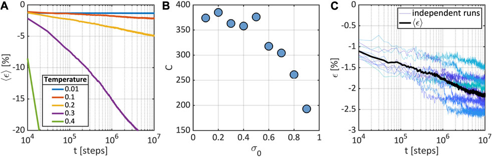
We use the term macroscopic response, to denote the response at the system level, as our simulations are conducted on bulk glasses. Conversely, microscopic response pertains to the dynamics of individual particles. Figure 2A shows the uniaxial strain evolution of the KA glass under a uniaxial compressive stress of ${\mathrm{\sigma }}_0=0.5$, and at different temperatures below ${\mathrm{T}}_{\mathrm{M}\mathrm{C}\mathrm{T}}$. The responses shown correspond each to the average over ten independent runs starting from different initial configurations of the glass. At the lowest temperature, the creep response is suppressed, at least over the duration of our simulations and the foreseeable future. In contrast, as the temperature nears the glass transition point, the system deforms significantly under the instantaneously applied uniaxial stress, and the strain increases dramatically fast (only a reduced range of strain is shown in Figure 2A). For the intermediate temperatures, the strain clearly shows a logarithmic dependence on time, $\epsilon \left(t\right)\propto \left({\sigma }_0/C\right)\log t+{\epsilon }_e$, where $C$ is the creep modulus, and ${\epsilon }_e$ is the initial elastic deformation of the glass under ${\sigma }_0$. This response is characteristic of primary creep where the rate of deformation decays inversely proportional to time, $\dot{\epsilon }\propto t^{-1}$. Figure 2B shows the effect of the stress ${\mathrm{\sigma }}_0$ on the creep modulus of the KA glass at $\mathrm{T}=0.1$. The creep modulus remains approximately constant for stress levels below approximately $0.5$, suggesting that inertial effects on the macroscopic mechanical response of the glasses resulting from the instantaneous application of the compressive stress are unimportant for ${\mathrm{\sigma }}_0\le 0.5$. In Figure 2C, we show the evolution of uniaxial strain for ${\mathrm{\sigma }}_0=0.5$ and $\mathrm{T}=0.1$, for each of the ten independent runs starting from different initial glass configurations (shades of blue), as well as the average response (black). The primary creep response of the glass is not only obvious for the average, but also evident in the individual responses, despite the presence of significant fluctuations, which can be attributed to the relatively modest size of the systems simulated.

FIGURE 2

FIGURE 2. Macroscopic creep response of the KA glass from MD simulations. (A) Time evolution of the average strain over ten independent runs, $〈\epsilon 〉$, for a compressive stress of ${\mathrm{\sigma }}_0=0.5$, and at different temperatures $\mathrm{T}=0.01$, $0.1$, $0.2$, $0.3$, and $0.4$. (B) Creep modulus of the KA glass at $\mathrm{T}=0.1$ as a function of ${\mathrm{\sigma }}_0$. (C) Strain evolution of each of the ten simulated systems at ${\mathrm{\sigma }}_0=0.5$ and $T=0.1$ (shades of blue) as well as the average response (black).

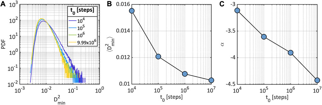
To characterize the microscopic response of the glasses during creep at ${\mathrm{\sigma }}_0=0.5$ and $\mathrm{T}=0.1$, we calculated the non-affine squared displacements for each particle $i$, over a time interval from $t_o$ to $t_o+∆t$: $D_{\min }^2\left(i,t_o,∆t\right)$. Non-affine displacements are particularly useful as they are associated to local plastic rearrangements. As discussed in the Section 2, this analysis is done using only optimized configurations of the glasses, which are outputted every ${10}^4$ steps during the simulations. In Figure 3A, we show, in the log-log scale, the distributions of non-affine displacements for ${∆t=10}^4$ steps, and taken at different times throughout the simulation, $t_o={10}^4$, ${10}^5$, ${10}^6$, and ${9.99\times 10}^6$ steps. The distributions incorporate data from all ten simulated systems. First, it is evident that, regardless of $t_o$, all the distributions display long, power-law tails to the right. These long-tails are strong evidence of the existence of a small number of particles that undergo plastic rearrangements during $∆t$. The power-law structure of the tails likely emerges from the convolution of the myriad of distinct particle environments in the glass which lead to as many characteristic relaxation timescales. With the progression of time (blue to yellow in Figure 3A), the average non-affine squared displacement $〈D_{\min }^2〉$ trends towards lower values (Figure 3B), and decay of the power-law tail becomes steeper, as shown by the evolution of the scaling exponent, $\mathrm{P}\mathrm{D}\mathrm{F}\propto D_{\min }^{2-\alpha }$, shown in Figure 3C. Therefore, both the average and extreme non-affine displacements appear to shift towards lower values as creep progresses. Interestingly, the scaling exponent of the power-law tail decreases logarithmically in time, analogous to the creep strain. This suggests that the tail of the distributions of non-affine displacements contain information about the creep response of the glass.

FIGURE 3

FIGURE 3. Microscopic creep response of the KA glass from MD simulations. (A) The probability distribution of non-affine squared displacements, $D_{\min }^2$, calculated over a time interval $∆t={10}^4$ steps at different times, $t_o$, during the simulations. (B) Average non-affine squared displacement $〈D_{\min }^2〉$ over time. (C) Scaling exponent of the power-law tail, $\alpha$, as a function of time.

3.2 Understanding the effect of $D_{\min ,0}^2$ and $∆t$ on accuracy of the ML predictions

Two key parameters, $D_{\min ,0}^2$ and $∆t$, determine whether a particle is classified as loose or tight. The choice of these parameters will, therefore, directly impact the quality of the dataset, and subsequently the accuracy of the ML predictions. While the long-tails in the probability distributions of $D_{\min }^2$ are strong evidence of the existence some particles that undergo plastic rearrangements, it is worth noting that there is no well-defined threshold, $D_{\min ,0}^2$, that can be used to unequivocally identify them, given the continuous nature of the distribution. The time interval over which the non-affine displacement in measured, $∆t$, is also critical, but its effect has not been investigated or discussed in previous studies. In this section, we investigate the effect of $D_{\min ,0}^2$ and $∆t$ on the accuracy of a classification model aimed at predicting whether or not a particle will undergo a plastic rearrangement ($D_{\min }^2>D_{\min ,0}^2$) over some time interval $∆t$.

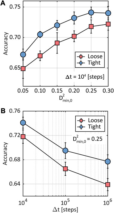
Figure 4 shows the validation accuracy for each class of classification models trained as described in the Section 2. Both Figures 4A, B show that the model performs slightly better on the majority class, which is expected given a series of factors including information richness and sampling quality. It is worth noting that the datasets used for training and validation, but not testing, were balanced using random undersampling. In Figure 4A, we see that the accuracy of the models increases monotonically with the threshold $D_{\min ,0}^2$, but appears to plateau beyond $D_{\min ,0}^2=0.25$. This can be explained by considering that particles with larger $D_{\min }^2$ possess structural environments that are highly correlated to plastic rearrangements, while those with lower $D_{\min }^2$ exhibit environments that may lead to such rearrangements, but with lower probability. Therefore, more selective thresholds lead to datasets with more reliable labels for the minority class, which helps to enhance the accuracy of the model. The plateauing of the accuracy is likely due to a concurrent significant decrease in the instances of the minority class within the dataset (as shown in Supplementary Table S1), which constrains the ability of the model to effectively learn from this class.

FIGURE 4

FIGURE 4. Validation accuracy for each class as a function of: (A) $D_{\min ,0}^2$ for $∆t={10}^4$, and (B) $∆t$ for $D_{\min ,0}^2=0.25$. Both the average and standard deviation are shown, over the predictions of five models each trained on an independent balanced bootstrap sample.

Figure 4B shows a logarithmic decay of the model accuracy with increasing $∆t$. We attribute this drop in accuracy to the changes in the local environment of the particles over time, which, over extended periods, can lead to memory loss of the initial structural conditions. In other words, the structural evolution of the system weakens the correlation between the environment used for feature computation, and the future behavior that the ML model is striving to predict. The logarithmic dependence of the accuracy on $∆t$ can be explained by the fact that the structural evolution becomes increasingly slow during creep (i.e., increasingly longer periods of time are required to achieve a similar magnitude of structural reorganization). We hypothesize that for short enough $∆t$, the accuracy of the model would also decrease based on the following argument. Given a local structural environment, the time it takes for a particle to undergo a plastic rearrangement will follow a statistical distribution. For example, if the process is activated, the time it takes a particle to undergo a plastic rearrangement would follow a Poisson distribution with a rate given by $r={\omega }_0{e}^{-E_a/k_{b}T}$, where ${\omega }_0$ is an attempt frequency, $E_a$ is an activation barrier (presumably conditioned by the particle’s structural environment), and $k_{b}T$ is the thermal energy. If ∆t is so short that it doesn't encompass reasonable extremes of that distribution, then particles will be labeled as tight or class 0, even if the structural environment is correlated to plastic rearrangements over longer, more appropriate time scales. Further investigations will be required to validate this hypothesis. Based on our results, we use $∆t={10}^4$ steps and $D_{\min ,0}^2=0.25$ to label the particles in the dataset moving forward. As shown in Supplementary Figure S1, other evaluation metrics, including the AUC (Area Under the Curve), which measures the ability of the model to discriminate between classes at various thresholds, and the F1 score, which captures the balance between precision and recall, are consistent with the class-specific accuracy. The consistency across these metrics provides a more robust confirmation of the predictive capability of the model and suggests its generalizability and robustness.

3.3 Feature selection and physical interpretation of the most important features

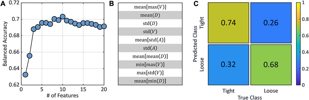
Before training the final classification ML model used to predict plastic rearrangements, we carry out RFE to identify and select the most important of the 60 features in the dataset. To this end, we use the data from the ten simulations at ${\mathrm{\sigma }}_0=0.5$ and $T=0.1$, where the examples were labeled using $∆t={10}^4$ and $D_{\min ,0}^2=0.25$. We perform RFE following the steps outlined in the Section 2. The testing balanced accuracy as a function of the number of top ranked features is shown in Figure 5A, which shows that the model accuracy peaks around the inclusion of 10 features, after which it experiences a slight gradual decrease in accuracy with the addition of more features. This decrease in accuracy can be attributed to various factors, including linear correlations between the features and the possibility of overfitting that arises from the increased complexity of the model.

FIGURE 5

FIGURE 5. (A) Average testing balanced accuracy versus the number of top n ranked features selected via RFE. Each point corresponds to the average of five model predictions trained each on independent balanced samples generated through random undersampling. (B) Top 10 ranked features by RFE. (C) Confusion matrix corresponding to the model trained using the top 10 ranked features by RFE, evaluated on the test set.

In Figure 5B, we show the top 10 ranked features by RFE, which will be used later to train the final model. The distribution between SRFs and MRFs is 4 to 6, suggesting that the medium-range order, which in the context of our work captures the interstitial environments of a particle’s neighbors (as determined by a Voronoi construction), plays a substantial role in determining plastic rearrangements. Interestingly, none of the selected SRFs—$\mathrm{S}\mathrm{t}\mathrm{d}\left(A\right)$, $\mathrm{S}\mathrm{t}\mathrm{d}\left(V\right)$, $\mathrm{S}\mathrm{t}\mathrm{d}\left(D\right)$, and $\mathrm{Min}\left(D\right)$—correspond to average quantities. The features related to the standard deviation encapsulate the variability in the particle’s local structural environment, whereas the minimum-related feature denotes an extreme of this environment. For example, a high standard deviation could suggest a high degree of heterogeneity in the structural environment, while a minimum could signify a limiting factor that precludes a plastic rearrangement. Overall, the selection of these SRFs suggests that the short-range structural heterogeneity and the distance to the closest neighbor play a significant role in the prediction of plastic events in KA glasses. Regarding the MRFs, 4 out of the 6 selected MRFs correspond to averages of SRFs related to non-mean summary statistics. This suggests that across mid-range length scales, beyond the nearest neighbors, the average heterogeneity significantly influences the occurrence of plastic rearrangements. Notably, half of the selected MRFs are associated to the selected SRFs, specifically $\mathrm{S}\mathrm{t}\mathrm{d}\left(A\right)$, $\mathrm{S}\mathrm{t}\mathrm{d}\left(V\right)$, and $\mathrm{Min}\left(D\right)$, further underlining the importance of these structural variables in the predictive process. Overall, the majority of the selected features relate to distances and volumes, with only 2 out of 10 related to areas. The prominence of distances may reflect the influence of local spatial configurations or the connectivity of the glass, when conceptualized as a graph. The significance of volume-based features could be indicative of the importance of local density fluctuations.

3.4 Predicting creep using the ML derived structural indicator looseness

As detailed in the Section 2, we apply the EasyEnsemble algorithm with logistic regression as the estimator, using random under-sampling to balance the dataset, to train a ML model that predicts the probability of a particle to be classified as loose or class 1 within the system. We refer to this prediction metric as looseness, $\mathbb{L}$, which, unlike previous machine learning-derived descriptors, such as softness (Cubuk et al., 2015; Cubuk et al., 2017; Liu et al., 2021), is bounded: $\mathbb{L}\in \left[\mathrm{0,1}\right]$. The balanced accuracy of the model stands at 71.6% for the (balanced) training set and 70.7% for the (unbalanced) testing set, which is comparable to the accuracy reported in previous studies (Liu et al., 2021). The close values between training and testing accuracies indicate that our model is generalizing well, being able to classify correctly over 70% of previously unseen particles (Figure 5C). Specifically, the model achieved an accuracy of 67.9% for the minority class of loose particles and 73.5% for the majority class of tight particles. Additionally, the AUC for the test set balanced using random undersampling is 0.772. The F1 score, calculated for each label and averaged with weighting based on the number of true instances for each label in the test set, is 0.848.

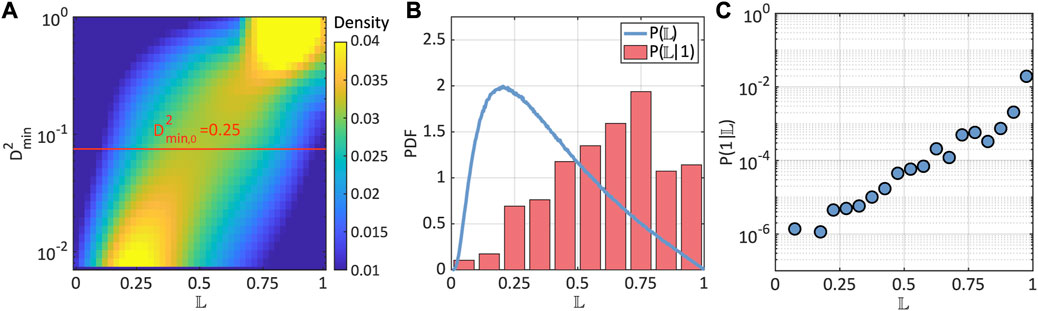
Figure 6A shows the probability density of particles as a function of the squared non-affine displacements, $D_{\min }^2$, and the predicted looseness, $\mathbb{L}$. This diagram was created as follows: for each interval in $D_{\min }^2$, we calculated the probability density of the looseness of all the particles in the dataset with squared non-affine displacements within that range. It is clear that the loose or tight populations of particles are well discriminated in the plane defined by $D_{\min }^2$ and $\mathbb{L}$, with the loose and tight particles being characterized by high and low $\mathbb{L}$ values, respectively. Our results demonstrate that the thresholds used to label particles, namely, $D_{\min ,0}^2=0.25$ and $\mathbb{L}=0.5$, effectively serve to separate and classify the particles as loose or tight (Figure 6A). Figure 6B shows the probability density of looseness for all particles, $p\left(\mathbb{L}\right),$ (blue line), as well as the conditional probability of looseness for just the loose or class 1 particles, $p\left(\mathbb{L}\left|1\right.\right)$ (bars). The overall distribution, which captures the underlying unbalanced character of the data set, shows that most of the particles as classified as tight, with the bulk of the looseness predictions being from about $\mathbb{L}=0.1$ to $0.4$. For $\mathbb{L}>0.5$, $p\left(\mathbb{L}\right)$ decays close to linearly. The conditional probability $p\left(\mathbb{L}\left|1\right.\right)$ reveals that about 71% of particles labeled as loose are assigned $\mathbb{L}>0.5$ by the model, which is, as it should, consistent with the accuracy of the model. The conditional probability of $\mathbb{L}$ given that a particle has been labeled as loose, $p\left(1\left|\mathbb{L}\right.\right)$, follows an approximately exponential relation with $\mathbb{L}$ (Figure 6C), which means that it is increasingly unlikely for a particle labeled as loose to be assigned a low $\mathbb{L}$ by the model. For example, there is a one in a million chance for a particle labeled as loose to receive a looseness assignment of 0.2 from the model. It is worth noting that because $\mathbb{L}\in \left[\mathrm{0,1}\right]$ is bounded, we expect the exponential relationship to break down for values of $\mathbb{L}$ near the boundaries.

FIGURE 6

FIGURE 6. Probability distributions of looseness, $\mathbb{L}$. The statistics shown correspond to predictions and labels of the entire dataset (training plus testing). (A) Probability density of particles as a function of the squared non-affine displacements, $D_{\min }^2$, and their predicted looseness, $\mathbb{L}$. The threshold $D_{\min ,0}^2=0.25$ used to label particles as loose or tight is shown in the plot as a horizontal red line. The results shown in this panel were smoothed out using a very light Gaussian filter. (B) Probability density of looseness for all particles, $p\left(\mathbb{L}\right),$ (blue line), as well as the conditional probability of looseness for just the loose particles (class 1), $p\left(\mathbb{L}\left|1\right.\right)$ (bars). (C) Conditional probability of looseness given particles labeled as loose, $p\left(1\left|\mathbb{L}\right.\right)$.

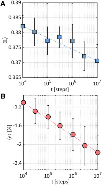
The time evolution of the average looseness in the glass, $〈\mathbb{L}〉$, where the angular brackets indicate ensemble average over all the particles in the glass, is shown in Figure 7A. The overall looseness of the system decreases as the glass creeps, which is consistent with the fact that the glass structure becomes less conducive to plastic rearrangements over time. Interestingly, this decrease in looseness approximately follows a logarithmic time dependence, $〈\mathbb{L}\left(t\right)〉\propto -\log t$, which is reminiscent of the evolution of the average macroscopic strain (Figure 7B): $〈\epsilon \left(t\right)〉\propto -\log t$. Our results suggest that $\mathbb{L}$, a machine-learned local descriptor based on simple, interpretable structural quantities, not only serves as an effective tool to predict microscopic plastic rearrangements in the KA glass during creep, but its ensemble-average, $〈\mathbb{L}〉$, correlates with the macroscopic creep response of the glass.

FIGURE 7

FIGURE 7. Time evolution of (A) the average looseness, and (B) the macroscopic strain response of the KA glass. Each point and its corresponding error bars represent the average and standard deviation, respectively, at each time, over the ten independent MD runs.

3.5 Fluctuations, and spatial and temporal autocorrelations of looseness

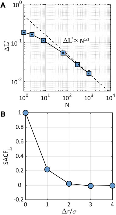
We characterize the scaling of the fluctuations of the looseness field as a function of system size, $\Delta {\mathbb{L}}^{*}\left(N\right)$, as described in the Section 2. Figure 8A shows that, overall, as the system size increases, the fluctuations become smaller. It is worth noting that for a size equal to the entire simulated system (i.e., $N=\mathrm{8,000}$), the fluctuations will become (artifactually) zero, which implies that our analysis is only valid for $N\le \mathrm{8,000}$. It is well established from equilibrium statistical mechanics that the fluctuations on thermodynamics properties scale with system size as $\propto N^{-1/2}$. We observe that for $N\ge {10}^2$, $\Delta \mathbb{L}$ scales in a manner similar to equilibrium fluctuations in relation to system size, which is somewhat unexpected considering the non-equilibrium nature and heterogeneity of the glasses. The space autocorrelation of $\mathbb{L}$, ${\mathrm{S}\mathrm{A}\mathrm{C}\mathrm{F}}_{\mathbb{L}}\left(\Delta r\right)$, shown in Figure 8B reveals short-range spatial correlations only, with a decay length scale of $\sim 0.63\sigma$. Beyond that, spatial correlations are lost, which is consistent with the lack of long-range order in the KA glass.

FIGURE 8

FIGURE 8. (A) Fluctuations of looseness field, $\Delta {\mathbb{L}}^{*}$, as a function of system size given by the number of particles, $N$. (B) Space autocorrelation function of $\mathbb{L}$, ${\mathrm{S}\mathrm{A}\mathrm{C}\mathrm{F}}_{\mathbb{L}}\left(\Delta r\right)$.

As described in the Section 2, in order to characterize the temporal autocorrelations, ${\mathrm{T}\mathrm{A}\mathrm{C}\mathrm{F}}_{{\mathbb{L}}^{*}}\left(\Delta t\right)$, we discretize space into voxels and map the looseness of individual particles to each voxel. That transformation allows us to track the time correlations of the looseness field, ${\mathbb{L}}^{*}\left(\mathbf{r},t\right)$, in a reference frame that does not depend on the ever evolving position of individual particles. The ${\mathrm{T}\mathrm{A}\mathrm{C}\mathrm{F}}_{{\mathbb{L}}^{*}}\left(\Delta t\right)$, shown in Figure 9A characterized by a very sharp drop over the first time interval due to the relatively large random fluctuations of looseness between consecutive configurations outputted for analysis. If one subtracts this effect, the ${\mathrm{T}\mathrm{A}\mathrm{C}\mathrm{F}}_{{\mathbb{L}}^{*}}$ decays over $\Delta t\approx 2\times {10}^6$ steps, after which it becomes slightly negatively correlated, and finally it slowly decorrelates over the timescale of the simulation (i.e., ${10}^7$ steps). The reason for the negative correlation observed in Figure 9A, can be explained based on the evolution of looseness at the single voxel level (an example is shown in Figure 9B), which does not gradually change over time, but rather undergoes sudden changes in values. A careful look at the time autocorrelation of individual voxels in space, ${\mathrm{T}\mathrm{A}\mathrm{C}\mathrm{F}}_{{\mathbb{L}}^{*}}^i$, reveals that the response is highly heterogeneous (Figure 9C), and therefore the average correlation shown in Figure 9A does not reveal the full picture. We observe that some voxels, the decay time scale is almost instantaneous, while for other it lasts over $2$ to $4\times {10}^6$ steps (Figure 9B). We quantify the heterogeneity in the relaxation time scales in Figure 9D, where we plot the probability distribution of times at which the ${\mathrm{T}\mathrm{A}\mathrm{C}\mathrm{F}}_{{\mathbb{L}}^{*}}$ for individual voxels crosses zero, $t_C=\Delta t\left({\mathrm{T}\mathrm{A}\mathrm{C}\mathrm{F}}_{\mathbb{L}}=0\right)$. We observe a clear power-law distribution of correlation time scales, with an exponent close to $-1$. We also observe a limit to the power-law behavior at $t_C^{*}\approx 3\times {10}^6$ steps, beyond which the probability of observing the looseness of a given voxel decorrelating slower than that quickly becomes null. It is likely that $t_C^{*}$ depends on the particular glass model and loading conditions, ${\mathrm{\sigma }}_0$ and $T$.

FIGURE 9

FIGURE 9. (A) Time autocorrelation function of the looseness field, ${\mathrm{T}\mathrm{A}\mathrm{C}\mathrm{F}}_{{\mathbb{L}}^{*}}\left(\Delta t\right)$. (B) Example of the evolution of looseness for a select voxel. (C) Time autocorrelation function of the looseness field, ${\mathrm{T}\mathrm{A}\mathrm{C}\mathrm{F}}_{{\mathbb{L}}^{*}}^i\left(\Delta t\right)$, for some individual voxels. (D) Probability distribution of the relaxation timescales of looseness for individual voxels, $t_C=\Delta t\left({\mathrm{T}\mathrm{A}\mathrm{C}\mathrm{F}}_{\mathbb{L}}=0\right)$.

4 Conclusion

In this study, we used a machine-learning (ML) classification model based on logistic regression trained with data from molecular dynamics (MD) simulations of Kob-Andersen (KA) glasses to derive a local structural descriptor, termed looseness, $\mathbb{L}$, which highly correlates with the propensity of particles to undergo plastic rearrangements during creep. Unlike other ML-derived structural descriptors such as softeness (Cubuk et al., 2015; Liu et al., 2021), looseness is based on straightforward, interpretable features and yields a real probability bound between 0 and 1. Our model can predict with an accuracy exceeding 70% whether an unseen particle within a KA glass will undergo a plastic rearrangement within a certain time interval. We showed that the evolution of the average looseness of the glass system, $〈\mathbb{L}〉$, mirrors the logarithmic time dependence observed in creep strain. This correlation highlights the link our model is able to establish between the microscopic dynamics at the single particle level over short time scales and the long-term macroscopic creep response of the KA glass. Our feature importance analysis revealed that none of the selected Short Range Features (SRFs) correspond to average quantities. Rather, features related to the extremal summary statistics of the interstitial structural environment dominate, emphasizing the critical role of short-range structural heterogeneity in predicting plastic rearrangements in KA glasses. Moreover, over half of the most important features were associated to the medium-range structural order of the glass, which highlights the importance of this length scale in predicting plastic rearrangements. Furthermore, our analysis of the spatial correlations of looseness revealed correlations only up to the medium-range length scale, beyond which the correlations die off–a finding that aligns with the lack of long-range order typical of the KA glass. Our examination of the temporal correlations of looseness unveiled a power-law distribution of relaxation timescales, which is reminiscent of the dynamic heterogeneity often postulated for glassy systems (Flenner and Szamel, 2010).

In conclusion, our research underscores the substantial predictive power of ML-derived structural indicators in systems experiencing concurrent stress and thermal excitations. Nonetheless, future research will be required to untangle the intricate interplay between thermal fluctuations and mechanical activation of structural defects in disordered solids, and how each contributes to the overall mechanical behavior of the system.

Data availability statement

The raw data supporting the conclusion of this article will be made available by the authors, without undue reservation.

Author contributions

MW: Methodology, Software, Visualization, Writing–Original draft. LR: Conceptualization, Methodology, Software, Supervision, Writing–Original draft.

Funding

The author(s) declare that no financial support was received for the research, authorship, and/or publication of this article.

Conflict of interest

The authors declare that the research was conducted in the absence of any commercial or financial relationships that could be construed as a potential conflict of interest.

Publisher’s note

All claims expressed in this article are solely those of the authors and do not necessarily represent those of their affiliated organizations, or those of the publisher, the editors and the reviewers. Any product that may be evaluated in this article, or claim that may be made by its manufacturer, is not guaranteed or endorsed by the publisher.

Supplementary material

The Supplementary Material for this article can be found online at: https://www.frontiersin.org/articles/10.3389/fmats.2023.1272355/full#supplementary-material

References

Ashwin, S. S., and Sastry, S. (2003). Low-temperature behaviour of the kob–andersen binary mixture. J. Phys. 15 (11), S1253–S1258. doi:10.1088/0953-8984/15/11/343

CrossRef Full Text | Google Scholar

Bapst, V., Keck, T., Grabska-Barwińska, A., Donner, C., Cubuk, E. D., Schoenholz, S. S., et al. (2020). Unveiling the predictive power of static structure in glassy systems. Nat. Phys. 16 (4), 448–454. doi:10.1038/s41567-020-0842-8

CrossRef Full Text | Google Scholar

Barber, C. B., Dobkin, D. P., and Huhdanpaa, H. (1996). The Quickhull algorithm for convex hulls. ACM Trans. Math. Softw. 22 (4), 469–483. doi:10.1145/235815.235821

CrossRef Full Text | Google Scholar

Bazant, Z. P., and Wittmann, F. H. (1982). Creep and shrinkage in concrete structures. United States: Wiley.

Google Scholar

Bell, R. L., and Langdon, T. G. (1967). An investigation of grain-boundary sliding during creep. J. Mater. Sci. 2 (4), 313–323. doi:10.1007/BF00572414

CrossRef Full Text | Google Scholar

Bishop, C. M., and Nasrabadi, N. M. (2006). Pattern recognition and machine learning. Berlin, Germany: Springer.

Google Scholar

Boattini, E., Marín-Aguilar, S., Mitra, S., Foffi, G., Smallenburg, F., and Filion, L. (2020). Autonomously revealing hidden local structures in supercooled liquids. Nat. Commun. 11 (1), 5479. doi:10.1038/s41467-020-19286-8

PubMed Abstract | CrossRef Full Text | Google Scholar

Brinson, L. C., and Gates, T. S. (1995). Effects of physical aging on long term creep of polymers and polymer matrix composites. Int. J. Solids Struct. 32 (6–7), 827–846. doi:10.1016/0020-7683(94)00163-q

CrossRef Full Text | Google Scholar

Castellero, A., Moser, B., Uhlenhaut, D., Dalla Torre, F., and Löffler, J. F. (2008). Room-temperature creep and structural relaxation of Mg–Cu–Y metallic glasses. Acta Mater. 56 (15), 3777–3785. doi:10.1016/j.actamat.2008.04.021

CrossRef Full Text | Google Scholar

Cubuk, E. D., Ivancic, R. J. S., Schoenholz, S. S., Strickland, D. J., Basu, A., Davidson, Z. S., et al. (2017). Structure-property relationships from universal signatures of plasticity in disordered solids. Science 358 (6366), 1033–1037. doi:10.1126/science.aai8830

PubMed Abstract | CrossRef Full Text | Google Scholar

Cubuk, E. D., Schoenholz, S. S., Rieser, J. M., Malone, B. D., Rottler, J., Durian, D. J., et al. (2015). Identifying structural flow defects in disordered solids using machine-learning methods. Phys. Rev. Lett. 114 (10), 108001. doi:10.1103/PhysRevLett.114.108001

PubMed Abstract | CrossRef Full Text | Google Scholar

Falk, M. L., and Langer, J. S. (1998). Dynamics of viscoplastic deformation in amorphous solids. Phys. Rev. E 57 (6), 7192–7205. doi:10.1103/PhysRevE.57.7192

CrossRef Full Text | Google Scholar

Fan, Z., Ding, J., and Ma, E. (2020). Machine learning bridges local static structure with multiple properties in metallic glasses. Mater. Today 40, 48–62. doi:10.1016/j.mattod.2020.05.021

CrossRef Full Text | Google Scholar

Flenner, E., and Szamel, G. (2010). Dynamic heterogeneity in a glass forming fluid: susceptibility, structure factor, and correlation length. Phys. Rev. Lett. 105 (21), 217801. doi:10.1103/physrevlett.105.217801

PubMed Abstract | CrossRef Full Text | Google Scholar

Harper, J., and Dorn, J. E. (1957). Viscous creep of aluminum near its melting temperature. Acta Metall. 5 (11), 654–665. doi:10.1016/0001-6160(57)90112-8

CrossRef Full Text | Google Scholar

Herring, C. (2004). Diffusional viscosity of a polycrystalline solid. J. Appl. Phys. 21 (5), 437–445. doi:10.1063/1.1699681

CrossRef Full Text | Google Scholar

Kob, W., and Andersen, H. C. (1995). Testing mode-coupling theory for a supercooled binary Lennard-Jones mixture. II. Intermediate scattering function and dynamic susceptibility. Phys. Rev. E 52 (4), 4134–4153. doi:10.1103/PhysRevE.52.4134

PubMed Abstract | CrossRef Full Text | Google Scholar

Langdon, T. G. (2006). Grain boundary sliding revisited: developments in sliding over four decades. J. Mater. Sci. 41, 597–609. doi:10.1007/s10853-006-6476-0

CrossRef Full Text | Google Scholar

Larini, L., Ottochian, A., De Michele, C., and Leporini, D. (2008). Universal scaling between structural relaxation and vibrational dynamics in glass-forming liquids and polymers. Nat. Phys. 4 (1), 42–45. doi:10.1038/nphys788

CrossRef Full Text | Google Scholar

Lemaître, G., Nogueira, F., and Aridas, C. K. (2017). Imbalanced-learn: a Python toolbox to tackle the curse of imbalanced datasets in machine learning. J. Mach. Learn. Res. 18 (1), 559–563.

Google Scholar

Li, M.-X., Zhao, S.-F., Lu, Z., Hirata, A., Wen, P., Bai, H.-Y., et al. (2019). High-temperature bulk metallic glasses developed by combinatorial methods. Nature 569 (7754), 99–103. doi:10.1038/s41586-019-1145-z

PubMed Abstract | CrossRef Full Text | Google Scholar

Liu, H., Xiao, S., Tang, L., Bao, E., Li, E., Yang, C., et al. (2021). Predicting the early-stage creep dynamics of gels from their static structure by machine learning. Acta Mater. 210, 116817. doi:10.1016/j.actamat.2021.116817

CrossRef Full Text | Google Scholar

Liu, X. -Y., Wu, J., and Zhou, Z. -H. (2009). Exploratory undersampling for class-imbalance learning. IEEE Trans. Syst. Man, Cybern. Part B 39 (2), 539–550. doi:10.1109/TSMCB.2008.2007853

PubMed Abstract | CrossRef Full Text | Google Scholar

McLean, D. (1966). The physics of high temperature creep in metals. Rep. Prog. Phys. 29 (1), 1–33. doi:10.1088/0034-4885/29/1/301

CrossRef Full Text | Google Scholar

Nabarro, F. (1948). Deformation of crystals by the motion of single lonsin report of a conference on the strength of solids (bristol, UK). Phys. Soc. 75, 75–90.

Google Scholar

Pedregosa, F., Varoquaux, G., Gramfort, A., Michel, V., Thirion, B., Grisel, O., et al. (2011). Scikit-learn: machine learning in Python. J. Mach. Learn. Res. 12 (85), 2825–2830.

Google Scholar

Peng, Z.-H., Yang, Z.-Y., and Wang, Y.-J. (2021). Machine learning atomic-scale stiffness in metallic glass. Extreme Mech. Lett. 48, 101446. doi:10.1016/j.eml.2021.101446

CrossRef Full Text | Google Scholar

Richard, D., Ozawa, M., Patinet, S., Stanifer, E., Shang, B., Ridout, S. A., et al. (2020). Predicting plasticity in disordered solids from structural indicators. Phys. Rev. Mater. 4 (11), 113609. doi:10.1103/PhysRevMaterials.4.113609

CrossRef Full Text | Google Scholar

Schoenholz, S. S., Cubuk, E. D., Sussman, D. M., Kaxiras, E., and Liu, A. J. (2016). A structural approach to relaxation in glassy liquids. Nat. Phys. 12 (5), 469–471. doi:10.1038/nphys3644

CrossRef Full Text | Google Scholar

Tanguy, A., Mantisi, B., and Tsamados, M. (2010). Vibrational modes as a predictor for plasticity in a model glass. Europhys. Lett. 90 (1), 16004. doi:10.1209/0295-5075/90/16004

CrossRef Full Text | Google Scholar

Thompson, A. P., Aktulga, H. M., Berger, R., Bolintineanu, D. S., Brown, W. M., Crozier, P. S., et al. (2022). Lammps - a flexible simulation tool for particle-based materials modeling at the atomic, meso, and continuum scales. Comput. Phys. Commun. 271, 108171. doi:10.1016/j.cpc.2021.108171

CrossRef Full Text | Google Scholar

Wang, Q., Ding, J., Zhang, L., Podryabinkin, E., Shapeev, A., and Ma, E. (2020). Predicting the propensity for thermally activated β events in metallic glasses via interpretable machine learning. NPJ Comput. Mater. 6 (1), 194. doi:10.1038/s41524-020-00467-4

CrossRef Full Text | Google Scholar

Wang, Q., and Jain, A. (2019). A transferable machine-learning framework linking interstice distribution and plastic heterogeneity in metallic glasses. Nat. Commun. 10 (1), 5537. doi:10.1038/s41467-019-13511-9

PubMed Abstract | CrossRef Full Text | Google Scholar

Wang, Q., and Zhang, L. (2021). Inverse design of glass structure with deep graph neural networks. Nat. Commun. 12 (1), 5359. doi:10.1038/s41467-021-25490-x

CrossRef Full Text | Google Scholar

Weertman, J. (1983). Creep deformation of ice. Annu. Rev. Earth Planet. Sci. 11 (1), 215–240. doi:10.1146/annurev.ea.11.050183.001243

CrossRef Full Text | Google Scholar

Widmer-Cooper, A., Perry, H., Harrowell, P., and Reichman, D. R. (2008). Irreversible reorganization in a supercooled liquid originates from localized soft modes. Nat. Phys. 4 (9), 711–715. doi:10.1038/nphys1025

CrossRef Full Text | Google Scholar

Wu, Y., Xu, B., Zhang, X., and Guan, P. (2023). Machine-learning inspired density-fluctuation model of local structural instability in metallic glasses. Acta Mater. 247, 118741. doi:10.1016/j.actamat.2023.118741

CrossRef Full Text | Google Scholar

Xiao, S., Liu, H., Bao, E., Li, E., Yang, C., Tang, Y., et al. (2021). Finding defects in disorder: strain-dependent structural fingerprint of plasticity in granular materials. Appl. Phys. Lett. 119 (24), 241904. doi:10.1063/5.0068508

CrossRef Full Text | Google Scholar