 G. Tolooei Eshlaghi
 G. Egels2
 S. Benito
 M. Stricker
 A. Hartmaier
- 1Interdisciplinary Centre for Advanced Materials Simulation (ICAMS), Ruhr-Universität Bochum, Bochum, Germany
- 2Chair of Materials Technology, Institute for Materials, Ruhr-Universität Bochum, Bochum, Germany
Introduction: A full three-dimensional (3D) microstructure characterization that captures the essential features of a given material is oftentimes desirable for determining critical mechanisms of deformation and failure and for conducting computational modeling to predict the material’s behavior under complex thermo-mechanical loading conditions. However, acquiring 3D microstructure representations is costly and time-consuming, whereas 2D surface maps taken from orthogonal perspectives can be readily produced by standard microscopic procedures. We present a robust and comprehensive approach for such 3D microstructure reconstructions based on three electron backscatter diffraction (EBSD) maps from orthogonal surfaces of two-phase materials.
Methods: It is demonstrated that processing surface maps by spatial correlation functions combined with principal component analysis (PCA) results in a small set of unique descriptors that serve as a representative fingerprint of the 2D maps. In this way, the differences between surface maps of the real microstructure and virtual surface maps of a reconstructed 3D microstructure can be quantified and iteratively minimized by optimizing the 3D reconstruction.
Results: To demonstrate the applicability of the method, the microstructure of a metastable austenitic steel in the two-phase region, where austenite and deformation-induced martensite coexist at room temperature, was characterized and reconstructed. After convergence, the synthetic 3D microstructure accurately describes the experimental system in terms of physical parameters such as volume fractions and phase shapes.
Discussion: The resulting 3D microstructures represent the real microstructure in terms of their characteristic features such that multiple realizations of statistically equivalent microstructures can be generated easily. Thus, the presented approach ensures that the 3D reconstructed sample and the associated 2D surface maps are statistically equivalent.
1 Introduction
Material structure plays a vital role in driving all material innovation efforts aimed at improving material properties and performance. The three-dimensional (3D) characterization of microstructures is oftentimes desirable to capture the essential features of a given material and to determine critical mechanisms of deformation and failure. Using 3D microstructures is also essential to conduct computational modeling to predict the material’s behavior under thermo-mechanical loading conditions (Benito et al., 2019). However, acquiring 3D microstructure representations is costly and time-consuming because standard microscopic procedures can only produce 2D surface maps, even though the material is inherently three-dimensional. Current state-of-the-art methods for 3D microstructure characterization are serial sectioning techniques (Spowart, 2006; Zaefferer et al., 2008; Mücklich et al., 2018) or X-ray tomography (Echlin et al., 2012; Ebner et al., 2013; Wang et al., 2013). Both methods produce a truthful characterization of the 3D structure of an individual specimen but require a rather large effort both in sample preparation and in the software-based reconstruction of the 3D structure. Therefore, the lack of systematic ways for characterizing the 3D microstructure represents a significant challenge in materials science.
It is important to point out that the aforementioned direct 3D measurement techniques such as serial sectioning techniques or X-ray tomography yield a deterministic description of an instantiation of an individual microstructure and these methods are generally applied to very small sample sizes, which may raise doubts on the statistical significance of their representation of the microstructure being investigated. However, a truthful statistical representation of a material’s microstructure is essential to establish a link to bulk properties. Currently, most of the well-established homogenization theories use statistical measures of the microstructure to build structure-property links (Fullwood et al., 2008a; Baniassadi et al., 2012; Tabei et al., 2013). Hence, for such applications, a statistical representation of the microstructure is sufficient to predict the macroscopic properties of a sample (Balzani et al., 2014). Typically, characterizing a material in two dimensions using standard microscope procedures yield information on surface areas that are large compared to microstructural feature sizes, e.g., the grain size, with a reasonable effort. In consequence, linking of 2D statistical descriptions from surface maps to 3D statistics is a potentially powerful approach. Extensive research into this idea has been conducted, demonstrating that it is simple to collect relevant microstructure statistics from carefully chosen 2D sections in polycrystalline samples and to assemble them into 3D spatial statistics; the required effort, however, is orders of magnitude lower than that required to measure the material structure in 3D volumes (Mason and Adams, 1999; Gao et al., 2006; Fullwood et al., 2010). Furthermore, these studies have demonstrated that higher-order distribution functions characterizing the 3D material structure may be derived from data gathered in 2D sections using stereology theory. It is important to note that these prior attempts did not seek to reconstruct a 3D material microstructure using the obtained 3D microstructure statistics, but rather they focused on collecting the 3D microstructure statistics and directly applying them to estimate bulk properties (Adams and Field, 1992; Adams, 1993).
Nevertheless, reconstructing a statistically representative 3D microstructure facilitates property predictions using numerical simulation approaches. Unlike homogenization theories, which merely require the specification of proper microstructure statistics, the representative volume element (RVE) technique relies on the geometrical representation of 3D microstructures to apply numerical tools such as micromechanical simulations (Biswas et al., 2020a). The difficulty of statistical microstructure reconstruction is dependent on the particular microstructure statistics. For example, if one simply considers the volume fractions of the constituents’ local states or phases, also called 1-point spatial correlations, it is straightforward to produce reconstructions that reflect appropriate microstructure statistics. In other words, when starting with such a basic description, there are usually many potential reconstructions. Among the available resources for statistical microstructure reconstructions, DREAM3D (Rollett et al., 2004; Groeber and Jackson, 2014) and Kanapy (Biswas et al., 2020a; Biswas et al., 2020b) are noted here. They take as input scanning electron microscopy (SEM) or electron backscatter diffraction (EBSD) data from one to three orthogonal surface maps of a polycrystalline sample to generate a full 3D model of the microstructure. By representing each constituent grain as an ellipsoid, the microstructure will reflect selected statistics such as volume fraction, grain size and aspect ratio distributions, and crystallographic texture, including orientation distribution function (ODF) and misorientation distribution function (MODF) (Adams et al., 1993; Xu et al., 2014). Nonetheless, the lineal path function (Lu and Torquato, 1992), the cluster correlation function (Jiao et al., 2009), or the spatial n-point correlations are more preferred high-dimensional statistical descriptors (Jiao et al., 2007; Kalidindi et al., 2011). Also, integral descriptors such as Minkowski tensors have received considerable interest (Scheunemann et al., 2015).
To avoid making arbitrary choices of microstructure descriptors, the n-point spatial correlations can be used to select descriptors in a systematic approach (Fullwood et al., 2010; Kalidindi et al., 2011). Using this approach, the microstructure descriptors can be selected according to their expected significance in affecting the effective properties of the material (Garmestani et al., 2001; Saheli et al., 2005; Adams et al., 2012). Although one-point spatial correlations only contain volume fraction information, they have been successfully applied to reconstruct microstructures. 2-point spatial correlations not only account for the 1-point statistics but also integrate higher-order statistical descriptions (Baniassadi et al., 2012; Sheidaei et al., 2013). These studies often attempted two-dimensional reconstructions using all of the selected classes of n-point statistics. For instance, phase-recovery algorithms have been utilized to reconstruct 2D microstructures (Fullwood et al., 2008b). Additionally, Monte-Carlo approaches have been employed to reconstruct microstructures using obtained spatial correlations (Garmestani et al., 2009; Tabei et al., 2013). Typically, the evolution of a microstructure is determined by the minimization of an objective function that represents the differences between spatial correlations of the reconstructed and original microstructures. In this context, Seibert et al. developed a gradient-based optimization method for reconstructing 3D microstructures from 2D micrographs (Seibert et al., 2021b; 2021a). They defined the objective error function using a variety of microstructure descriptors like spatial correlations and Gram matrices. In their work, the chosen descriptors were differentiable with respect to the microstructure and a gradient-based optimization technique was applied to minimize the error function. Additionally, Turner et al. (2016) utilized location and neighborhood histogram reweighting to develop a solid texture synthesis algorithm for microstructure reconstruction. This approach provides a means to generate statistically similar 3D microstructures in cases when only 2D measurements are possible. Furthermore, several data-driven microstructure reconstruction techniques using Generative Adversarial Networks (GANs) (Yang et al., 2018; Kench and Cooper, 2021) and Variational Autoencoders (VAEs) (Noguchi and Inoue, 2021; Zhang et al., 2021), have been presented. Although these techniques have low computing time, they require a training data set and can only reconstruct a microstructure from a specific point in the latent space, not a specific descriptor. Hence, the descriptors of a microstructure are represented by the latent space variables in a neural network. Furthermore, in the absence of a training data set, the transfer learning method has been employed for microstructure reconstruction (Li et al., 2018; Bostanabad, 2020). This approach has been also extended to incorporate 2-point statistics (Bhaduri et al., 2021).
In the present work, an alternative workflow is suggested to generate synthetic 3D two-phase microstructures resembling real ones in a statistical sense from 2D surface maps of three orthogonal surfaces. The applicability of the proposed method is demonstrated through the 3D reconstruction of microstructures of metastable austenitic steels in the two-phase region. For this purpose, a metastable austenitic steel, where austenite and deformation-induced
The paper is organized as follows: After this introduction, Section 2 presents the microstructure reconstruction workflow and the background and equations for accurately computing spatial correlations. Furthermore, a PCA-based low-dimensional representation of these statistical features is introduced. Thereafter, the definition of a suitable loss function that quantifies the differences between descriptors of the synthetic and experimental surface maps and the differential evolution optimization approach for minimizing the loss are presented. In Section 3, the applicability of the proposed workflow for the reconstruction of 3D samples is demonstrated for case studies on the 3D reconstruction of synthetic and experimental microstructures. The obtained results are summarized in Section 4.
2 Methods and workflow
This paper focuses on 3D reconstruction of two-phase materials based on three orthogonal surface maps. To demonstrate the applicability of the method, the microstructure of a metastable austenitic steel in the two-phase region, where austenite and deformation-induced
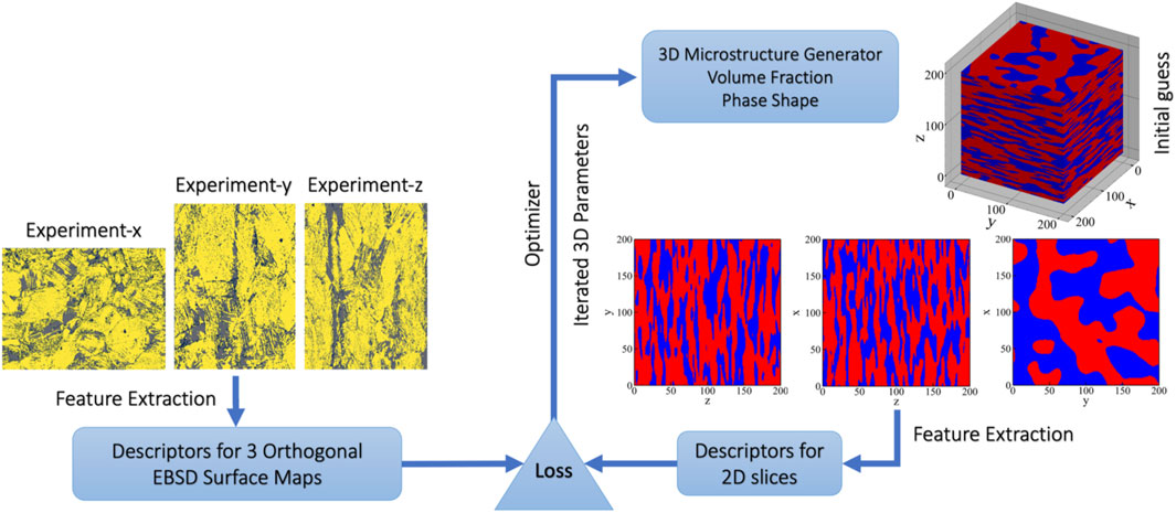
FIGURE 1. A schematic description of the workflow to reconstruct 3D microstructures from surface maps. The input is represented by three EBSD maps from orthogonal surfaces of a two-phase steel (yellow: martensite, gray: austenite) from which a low-dimensional, yet representative vector of descriptors is extracted. The corresponding descriptors are generated from a synthetic 3D microstructure (red: martensite, blue: austenite) such that a scalar loss function can be evaluated to assess the similarity between the surface maps of real and synthetic microstructures. In an iterative procedure, the parameters of the 3D microstructure generator are optimized such that the loss function becomes minimal. The microstructure generator tool from the open-source python package pyMKS is used to produce synthetic 3D microstructures (Brough et al., 2017).
The workflow in Figure 1 incorporates a microstructure generator tool from the open-source python package pyMKS to produce synthetic 3D two-phase microstructures based on physical parameters, such as volume fraction and phase shape (Brough et al., 2017). From the surfaces of a synthetic microstructure, 2D images are produced similar to the surface maps of the real material. Consequently, the reconstruction task is implemented as an optimization problem in which the synthetic 3D microstructure is iteratively modified until the difference between synthetic and experimental surface maps is minimized. The primary challenge in this optimization problem lies in defining a proper loss function to be minimal that quantifies the differences between surface maps in a physically sound yet numerically efficient way. We demonstrate that processing surface maps by spatial correlation functions, often referred to as 2-point statistics, and PCA results in a small set of unique descriptors that serve as a fingerprint of the 2D maps (Niezgoda et al., 2013). These descriptors encode the topological information of 2D maps in a compact format and can be used to characterize both experimental and synthetic surface maps. In this way, the differences between the two sets of surface maps can be quantified and iteratively minimized.
The 2D surface maps are analyzed using the 2-point statistics tool in pyMKS with the aid of computationally efficient Discrete Fourier Transformation-(DFT)-based approaches (Brough et al., 2017). While 2-point statistics provide visually intuitive representations of microstructures, they are very high dimensional. PCA, which is an effective dimensionality reduction approach that results in a small set of unique descriptors, is used to reduce the high dimensionality of the 2-point statistics representation. To obtain a set of 2D surface maps as the data basis for fitting the PCA, pyMKS is employed. In the following sub-sections, the context and equations for computing the 2-point spatial correlations, as well as a PCA-based, low-dimensional representation of these statistical features are presented. Subsequently, the differential evolution optimization strategy for minimizing the loss is described, along with the definition of an appropriate loss function that quantifies the differences between the descriptors of the synthetic and experimental surface maps. In this study, all reconstructions have a final volume size of 2003 voxels. The reconstruction size has been chosen to be small enough to be generated within the available computer resources, while still being large enough to ensure that enough of the microstructure’s features are captured in the reconstruction. All reconstructions are performed on a system with 64 GB of memory and Intel W-2255 10-core CPU.
2.1 Digital microstructure
For the mathematical representation of material microstructures, discretized representations have been widely employed (Adams et al., 2012). Specifically, in these cases, the most convenient representation of the microstructure is an array,
In this section, we generate a large dataset of voxelated 3D eigen microstructures, extract their 2D cross-sections, and quantify their 2-point correlations. PyMKS microstructure generator algorithms are used to generate 3D two-phase microstructures with a size of
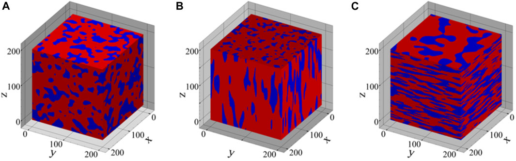
FIGURE 2. Three-dimensional synthetic microstructures with varying volume fractions (VF) and shapes of the secondary phase, including (A) equiaxed phase with VF = 0.3, (B) prolate phase with VF = 0.2, and (C) oblate phase with VF = 0.4.
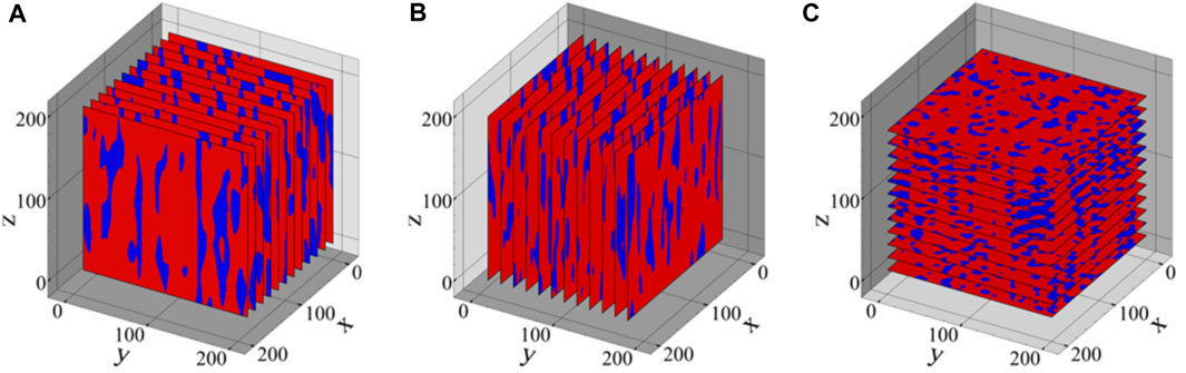
FIGURE 3. The data basis for the fitting of the PCA method is generated by producing 10 slices in (A) x-, (B) y-, and (C) z-direction of each 3D sample, here demonstrated for the microstructure shown in Figure 2B.
2.2 Microstructure statistics
Conventionally, the common practice has been to rely on intuitive metrics that reflect statistics of two-phase microstructures, such as the average elemental composition, phase volume fractions, lattice parameters, and averaged phase shape and orientation. These metrics provide simple representations of complex microstructures by several scalar quantities, thereby facilitating microstructure specification, comparison of effects of varying processing conditions, and incorporation of the microstructure into property prediction models. These measures, however, fail to account for critical higher-order statistical features and for a given set of values for these extremely low-dimensional properties, it is for most microstructures almost impossible to construct statistically similar instantiations of the original material structure, i.e., an inverse mapping from (several) scalar quantities is practically impossible. Consequently, we infer that these simple metrics fail to adequately capture the complexities of a real microstructure. Richer statistical descriptors, such as n-point spatial correlation functions, often known as n-point statistics, have a substantially larger dimensionality. Recent research has demonstrated that by combining the physics-inspired concept of n-point spatial correlations, combined with machine learning dimensionality reduction techniques such as PCA, a systematic and thorough quantification of a microstructure is achievable (Basu et al., 2022). The idea is to gather local neighborhood information in a systematic way around some chosen point in the microstructure. 1-point spatial correlations (i.e., n = 1) are the simplest n-point spatial correlations since they simply indicate the probability of observing a given local state of interest at a given spatial point in the material structure. Such basic statistics only capture the volume fraction of the various local states of a microstructure. 2-point statistics describe the first-order spatial correlations between the distinct constituent phases in the material. Hence, they provide a quantitative measure of neighborhood statistics by focusing on a pair of material points connected by a certain vector. In general, higher-order spatial correlations, i.e., 3-point spatial correlations and higher, are known to affect the effective characteristics; however, for the class of eigen microstructures investigated in this paper, it is expected that these correlations will have non-linear relationships with the 2-point spatial correlations (Mann and Kalidindi, 2022). Here, this will become clear from the fact that eigen microstructures will be reconstructed statistically from their 2-point spatial correlations. In the following, the quantitative framework for extracting these statistical features from 2D surface maps generated in the previous section is presented.
The 2-point spatial correlations, represented by
in which
Auto-correlations of the martensite and austenite phases and their cross-correlation function are computed for the generated 2D surface maps. Since
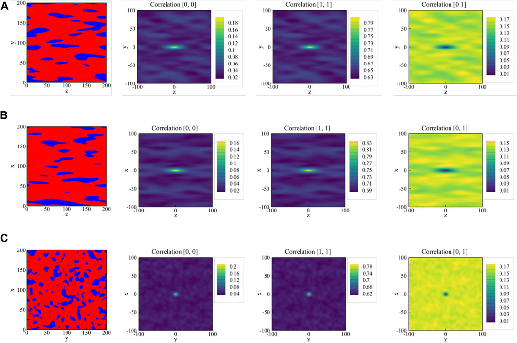
FIGURE 4. Middle planes in (A) x-, (B) y-, and (C) z-direction of the three-dimensional sample shown in Figure 2B (left column) and the associated 2D auto-correlation maps for austenite regions (second column), for martensite regions (third column), and the cross-correlation between the two phases (right column).
The potential advantages of using 2-point spatial correlations as the descriptors rather than the discrete microstructures have already been discussed. In this context, it is important to note that the features extracted via 2-point spatial correlations are capable to work as universal features for many relevant effective bulk material properties (Generale and Kalidindi, 2021). However, the correlation maps of a 2D image are high-dimensional representations of the microstructure. In Figure 4, each correlation map is a 2D array of size
2.3 Dimensionality reduction
In the classification of various and large datasets of microstructures and the development of data-driven PSP links, low-dimensional representations are of great use. PCA is an effective technique for dimensionality reduction which applies a linear and distance-preserving transformation of data to a new orthogonal basis that maximizes the variance captured in the data in the least number of terms corresponding to the new PC basis. PCs are a linear combination of the original components of the data. Consequently, the number of variables in the new basis, called PC scores, that are needed to adequately describe the data is often considerably lower than the number of original variables and the number of prominent variables in the new basis is determined by the desired explained variance in the dataset. Furthermore, PCA’s ability to preserve distance allows for quantitative relative comparisons of the data points. In Sections 2.1 and 2.2, we generated a large dataset of 2D voxelated eigen microstructures and computed their 2-point spatial correlations. Here, this dataset consisting of the correlation maps for the 2D images is utilized to train the PCA. Hence, inputs to the PCA established in this study are 2-point spatial correlations maps, which consist of 2D arrays of size
PCA provides an ordered orthogonal decomposition into PC basis, which allows for a typically handful of scalar PC scores to be used as the fingerprint of the surface maps. This method can be regarded as the identification of patterns (basis vectors) and then weighting of these patterns (PC scores), to effectively capture the variance in the 2-point spatial correlations of the microstructure dataset. Once these patterns and their scores have been determined, the 2-point statistics of the kth microstructure in the dataset (or a new microstructure to be added to the dataset) can be represented by the linear combination of the patterns (Niezgoda et al., 2011; Niezgoda et al., 2013),
where
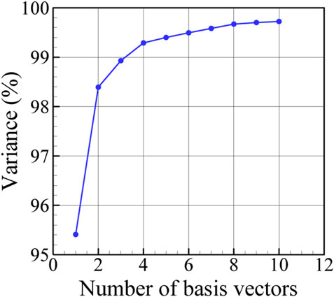
FIGURE 5. Explained variance in data in terms of the number of PC basis vectors used for the low-dimensional presentation.
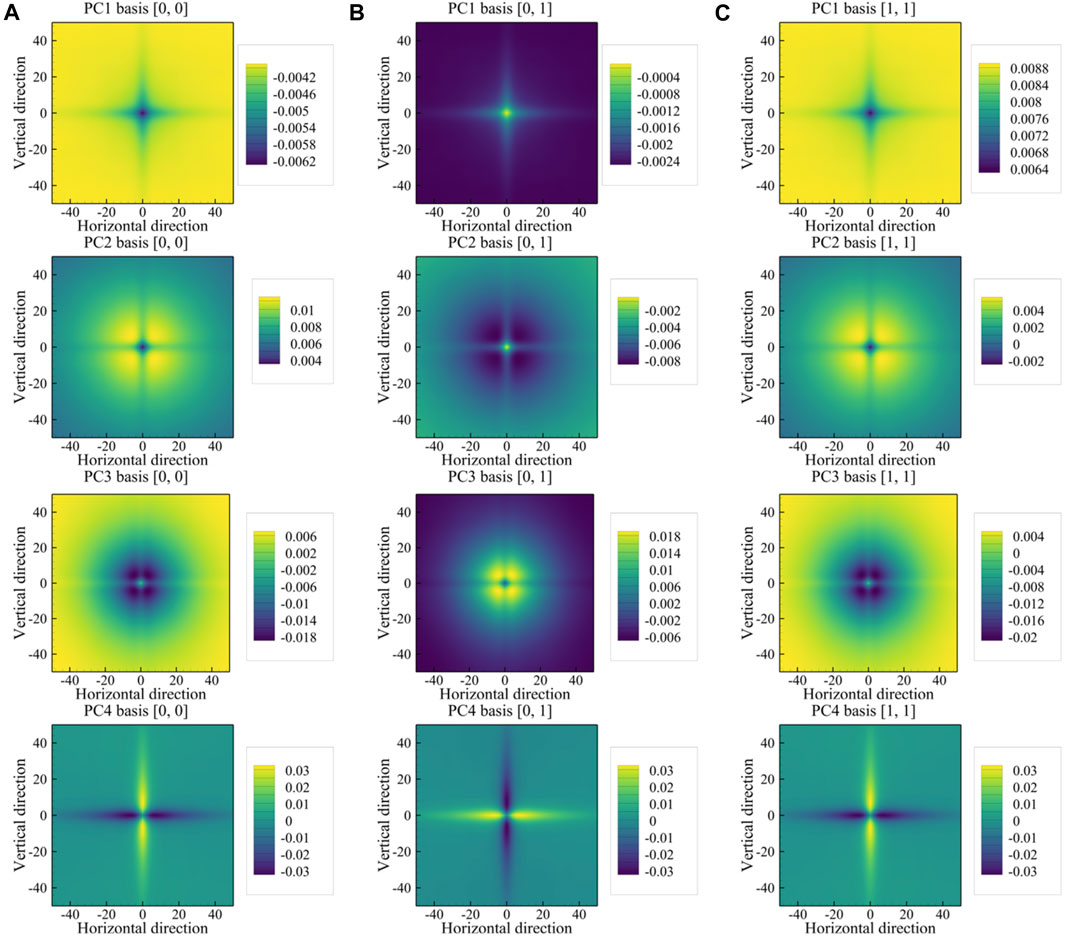
FIGURE 6. PC basis vectors for (A) auto-correlation for the austenite phase, (B) auto-correlation for the martensite phase, and (C) cross-correlation between the two phases. The rows from top to bottom correspond, in order, to the PC1, PC2, PC3, and PC4 basis vectors.
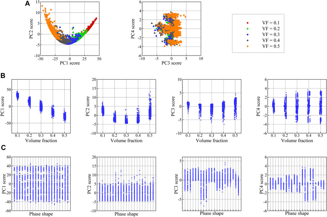
FIGURE 7. (A) Low-dimensional presentation (PC scores) of spatial correlation data, including PC1 against PC2 and PC2 against PC3 plots, and (B) the variation of PC1, PC2, PC3, and PC4 scores in terms of volume fraction and (C) the variation of PC1, PC2, PC3, and PC4 scores in terms of phase shape.
2.4 Loss function
Having chosen a small set of PC scores as the unique descriptors to characterize 2D surface maps, reconstructing a statistically equivalent 3D digitized microstructure is cast as an optimization problem by adjusting an initial 3D microstructure to minimize a loss function. The reconstruction workflow depicted in Figure 1 is based on this inverse procedure to first generate synthetic 3D microstructures using arbitrary physical parameters, and then to compare the resulting artificial surface maps to the corresponding real ones in descriptor space. Hence, the optimization seeks to update the 3D physical parameters, including volume fraction and phase shape, in a way that the average difference between the PC scores of the reconstruction and the PC scores of the reference images is minimized.
The mean squared error (MSE), which provides a quantitative measure of differences between the PC scores, serves as the basis for defining the loss function, hereafter denoted by
where
3 Applications
In this section, we examine the applicability and performance of the suggested microstructure reconstruction workflow. For this purpose, two classes of two-phase microstructures are considered. The first includes synthetic surface maps, digitally generated using pyMKS (Brough et al., 2017), while the second class contains experimental surface maps, acquired using EBSD measurements on metastable austenitic steels in the two-phase region (Egels et al., 2018).
3.1 Synthetic microstructure
The 3D microstructure reconstruction workflow is first validated using synthetic 2D surface maps obtained from the orthogonal surfaces of a reference two-phase 3D microstructure. For this purpose, the pyMKS microstructure generator is first employed to create a 3D microstructure with a volume fraction of 0.4 for the austenite regions and mean shape of 15, 45, and 100 voxels along the x, y, and z-axes, respectively; shown in Figure 8A. Afterwards, three surface maps are extracted from this microstructure. For this purpose, the 3D microstructure is digitally sectioned along three orthogonal planes, which are normal to the x-, y-, and z-axes. These orthogonal cross-sections of the 3D microstructure are used as input 2D reference images for the reconstruction procedure. These three orthogonal reference maps together with their autocorrelation map for austenite can be seen in Figures 8B–D. The variation of PC1 through PC5 as a function of area fraction is depicted in Figure 9 as scattered plots for the two-dimensional dataset images as well as for the generated synthetic reference images. In each plot, the gray point denotes the dataset images. Here, the first five PC scores are selected as the fingerprint of each image. Then, based on the proposed workflow described in Section 2, the three synthetic surface maps are used to reconstruct a statistically similar microstructure in three dimensions, which is then compared to the original 3D microstructure shown in Figure 8A.
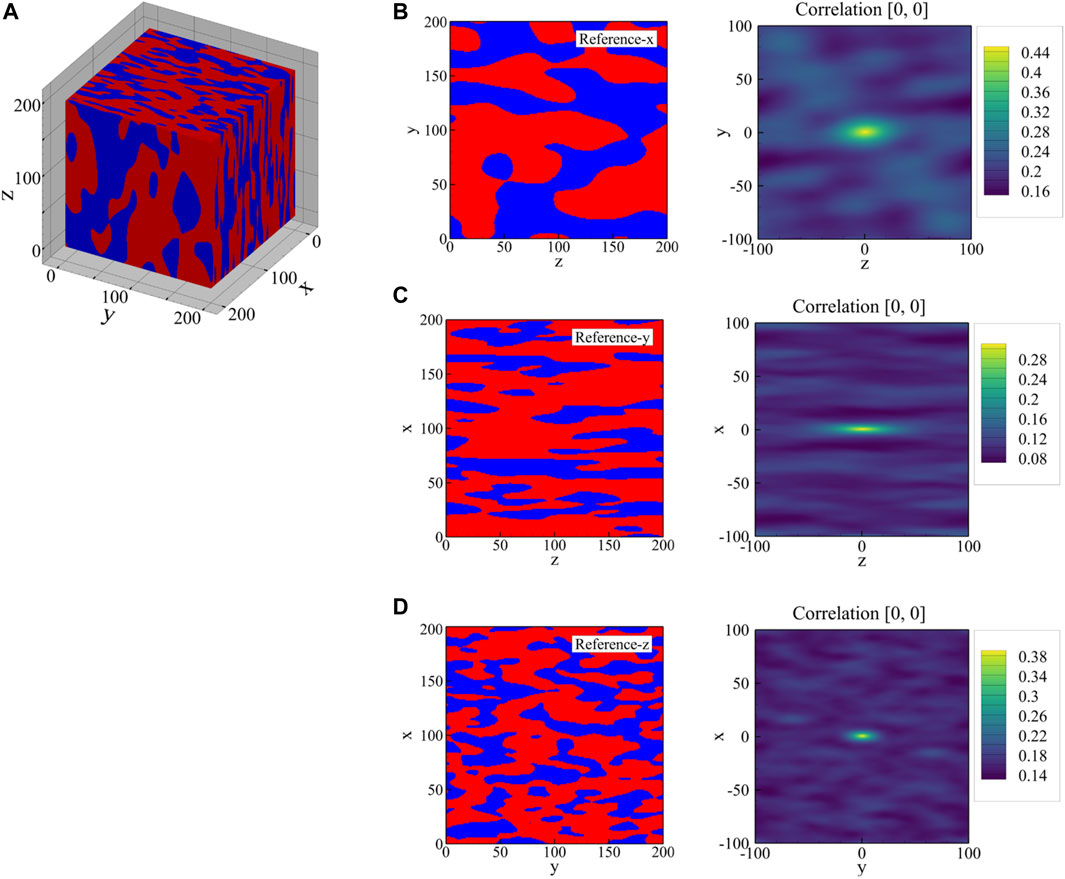
FIGURE 8. (A) The reference 3D microstructure, and its 2D cross-sections normal to the (B) x-, (C) y-, and (D) z-directions in the second column and their corresponding auto-correlation map for the austenite phase in the third column. The area fraction of the austenite phase is 0.46 in (A), 0.33 in (B), and 0.42 in (C), which corresponds to the highest central value in each auto-correlation map. The original 3D microstructure has a volume fraction of 0.396 and average phase shapes of 15, 45, and 100 voxels along the x-, y-, and z-axes, respectively.
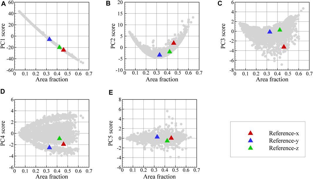
FIGURE 9. Variation of PC1 through PC5 scores in (A–E) as a function of area fraction for the dataset images and reference images. The gray points denote the values obtained from all images in the dataset used to generate the PC basis vectors shown in Figure 6.
The reconstructed microstructure shown in Figure 10A correspond to the minimum loss value plotted in Figure 10B. Furthermore, the evolution of physical parameters during optimization is illustrated in Figures 10C–F. The time required to reconstruct a 3D microstructure depends primarily on the reconstruction resolution, and in this case total reconstruction took around 5 h. The volume fraction of the austenite regions in the reconstructed 3D microstructure is 0.4 and its average shape is found to be 12, 46, and 105 voxels along the x-, y-, and z-axes. As can be seen in Figure 10B, the final loss value is not zero and reaches a minimum of 0.15 as a result of comparing the mean value of PC scores in 10 slices in each direction with the reference PC scores. If the number of slices in each direction used to define the loss function is increased, the final value of loss should decrease. As illustrated in Figure 10, once the loss minimization has been performed, the physical parameters of the reference 3D microstructure including the volume fraction of austenite regions and its mean phase shapes are accurately reproduced in the reconstructed 3D microstructure. The original values for the physical parameters of the reference 3D microstructure are shown as dashed red lines in Figures 10C–F. In these figures, the output of the differential evolution algorithm for each iteration is shown and it corresponds to the smallest loss value found up to that point during optimization. Although the reconstructed microstructure in Figure 10A is not identical to the reference microstructure in Figure 8A, they possess similar three-dimensional physical parameters and are statistically similar in terms of the first five PC scores. Hence, they can be regarded as two realizations of the same microstructure, sharing similar properties, but with different phase locations and shapes. Based on these results, we conclude that the five PC scores accurately reflect the important microstructural characteristics. Furthermore, each optimized 3D microstructure, with a loss value less than a chosen threshold, would be statistically similar to the reference microstructure in terms of the first five PC scores. As a result, the proposed workflow can be used to generate large databases of statistically similar synthetic microstructures.
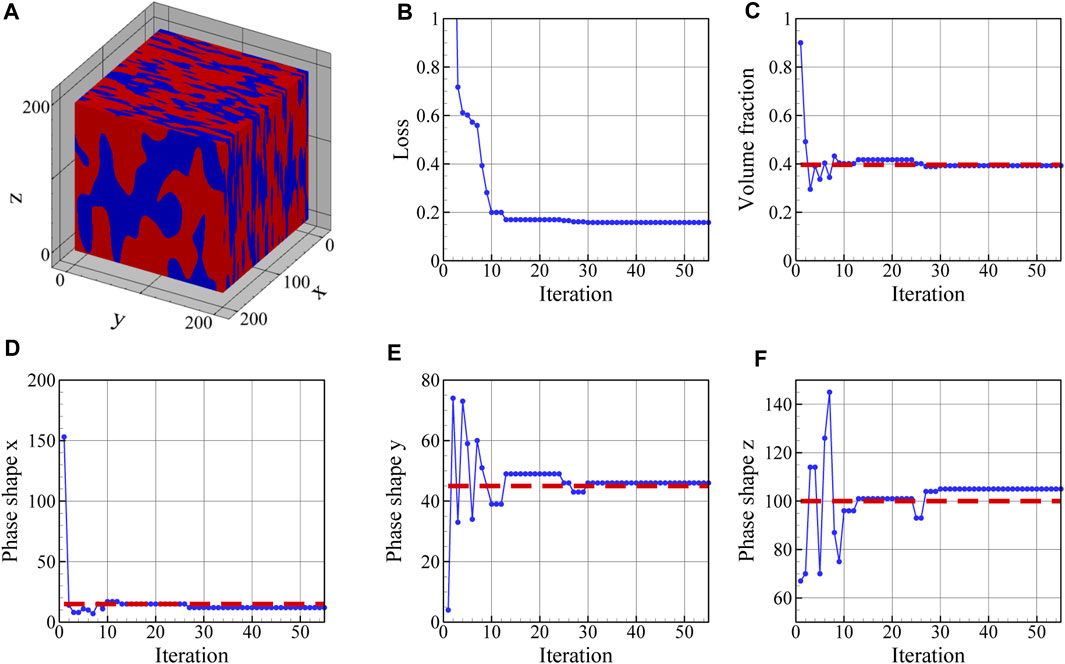
FIGURE 10. (A) Reconstructed 3D microstructure and the evolution of (B) loss function, (C) volume fraction, and phase shape along the (D) x-, (E) y-, and (F) z-direction during optimization. The reconstructed 3D microstructure has a volume fraction of 0.4 and phase of 12, 46, and 105 voxels along the x-, y-, and z-axes, respectively. The minimum value of the loss is 0.15. The red dashed lines in subfigures (C–F) indicates the parameter values that have been used to generate the reference microstructure shown in Figure 8A.
3.2 Experimental microstructure
After validating the reconstruction workflow in Section 3.1, its feasibility for use with experimental microstructures is explored in this section. Based on three experimental images from orthogonal surfaces of a metastable austenitic steel sample, the microstructure is reconstructed in three dimensions. For this purpose, three surface maps of this two-phase steel were produced with EBSD microscopy, which are illustrated in Figure 11. These three orthogonal surface maps were acquired from a deformed tensile specimen of AISI 304L type austenitic stainless steel. The examined specimen was a round tensile specimen with a diameter of 5 mm, which was plastically deformed at room temperature until failure at 61 % elongation. The chemical composition of the material is listed in Table 1.
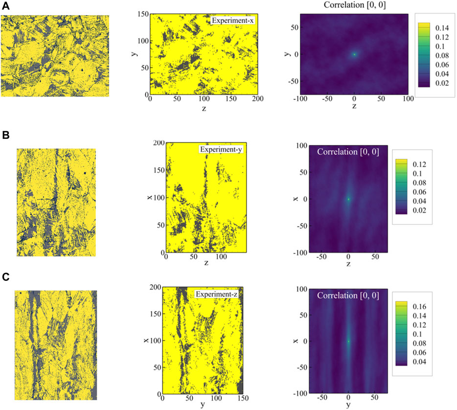
FIGURE 11. Original EBSD phase maps normal to the (A) x-, (B) y-, and (C) z-axes, the corresponding resized images, and the auto-correlation maps for the austenite phase (gray phase) are shown from left to right. The area fraction of the austenite phase in resized images is 0.15 in (A), 0.13 in (B), and 0.17 in (C), which corresponds to the maximum central value in each auto-correlation map. The original EBSD phase maps in (A), (B) and (C) have area fractions of 0.13, 0.11, and 0.15, respectively.
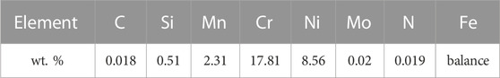
TABLE 1. Chemical composition of the examined material measured via optical emission spectroscopy. Values are in wt. %.
To investigate the microstructure in three orthogonal directions, three different samples were cut out of the fractured tensile specimen, of which two represent views orthogonal to the tensile axis and one represents the view parallel to the tensile axis. These EBSD phase maps can be seen in Figure 11, in which the x-axis corresponds to the tensile axis. The samples were embedded in a resin bond and then metallographically prepared by several steps of grinding and polishing with a diamond suspension. A final preparation step of vibratory polishing with colloidal SiO2 suspension was applied for 12 h to receive a sufficient surface quality for EBSD measurements. The EBSD measurements were performed using a field emission gun SEM MIRA3, equipped with a Nordlys Nano EBSD detector by Oxford Instruments. The SEM was operated at an acceleration voltage of 20 kV and a working distance of 17 mm with a 70° tilted sample holder. For each of the orthogonal views, a two-dimensional map with a size of
The resultant PC bases in Section 2.3 enable the transformation of the correlation maps associated with the three EBSD maps into the PC space. The 2-point spatial correlation maps used as input to the PCA are standardized as a
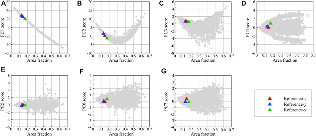
FIGURE 12. Variation of PC1 through PC7 scores in (A–G) as a function of area fraction for the dataset images and EBSD phase maps.
In Figure 13, the reconstructed 3D microstructure of the dual phase material based on the three orthogonal EBSD maps shown in Figure 11 is shown together with the convergence of the loss function and the physical microstructure descriptors. In this work, the effect of the number of 2D images in each direction on the accuracy of the reconstruction has not been examined. As can be seen in Figure 13B, the final loss value during optimization is not zero and reaches a minimum of 0.85 as a result of comparing the mean value of PC scores in 10 slices with the experimental PC scores in each direction. The depicted reconstructed microstructure in Figure 13A corresponds to the minimum loss value. This loss value can be reduced if we increase the number of slices in each direction used to define the loss function. The evolution of the physical parameters including austenite volume fraction and its mean shape along the x-, y-, and z-directions during the optimization procedure are illustrated in Figures 13C–F. After convergence, the volume fraction of austenite regions in the reconstructed 3D microstructure is 0.15 and its average shape is 12, 46, and 105 voxels along the x-, y-, and z-axes. After the optimization task, the mean value of PC1 through PC7 scores for ten slices normal to the x-, y-, and z-, directions converges to the corresponding experimental values. The evolutions of the first three averaged PC scores are depicted in Figure 14 for each direction. It is seen that, after convergence, the synthetic 3D microstructure in Figure 13A accurately describes the experimental system in terms of physical parameters including volume fraction (here: 15% austenite) and phase shapes (here: aspect ratio of 20:4:3 for austenite regions). Hence, the presented approach ensures that the 3D reconstructed sample and the associated 2D experimental EBSD maps are statistically equivalent.
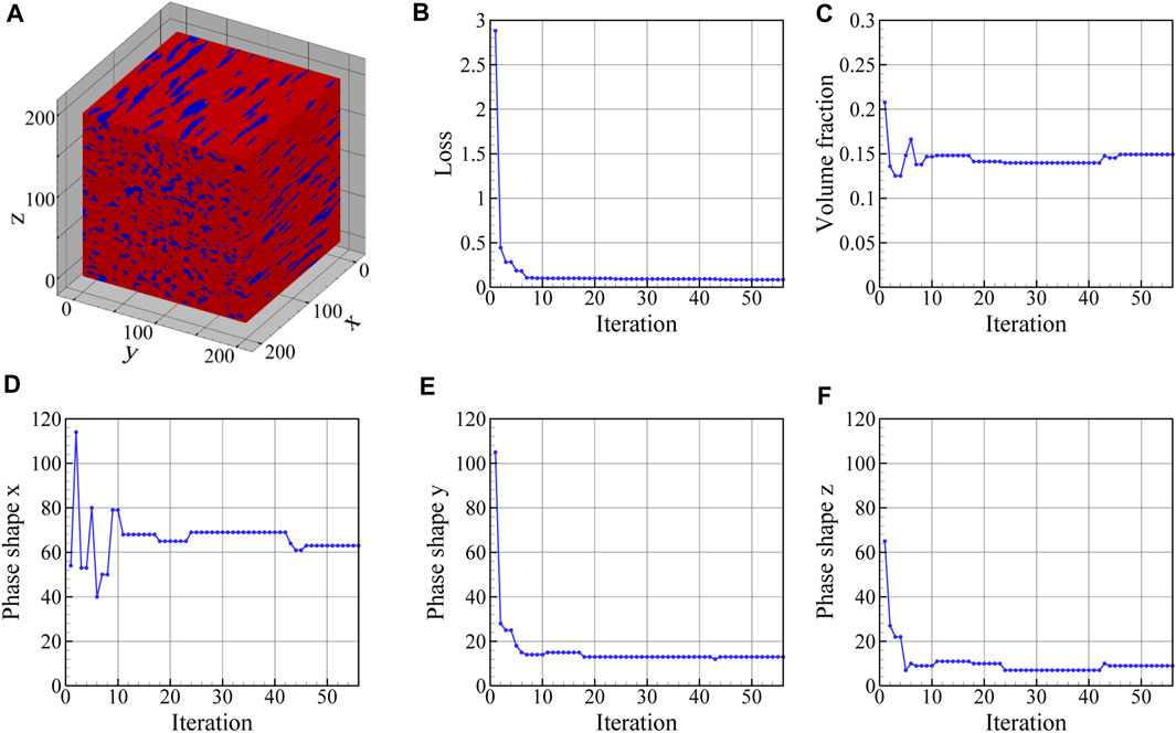
FIGURE 13. (A) The final 3D microstructure reconstructed from the experimental surface slices (see Figure 11), and the evolution of (B) loss function, (C) volume fraction, and phase shapes along the (D) x-, (E) y-, and (F) z-direction during the optimization procedure. The reconstructed 3D microstructure has a volume fraction of 0.15 and phase shapes of 63, 13, and 9 voxels along the x-, y-, and z-axes, respectively. The minimum value of the loss function is 0.085.
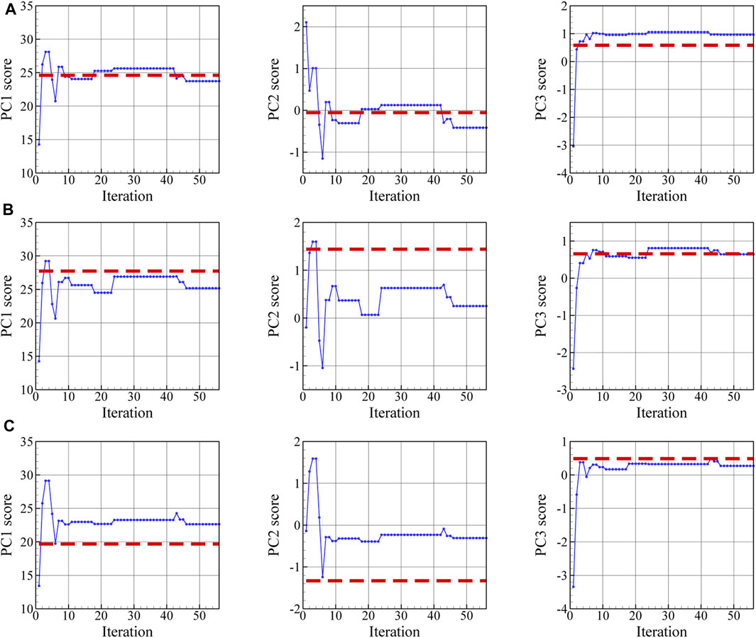
FIGURE 14. During optimization, the averaged value of PC1 through PC3 scores in slices normal to (A) x, (B) y-, and (C) z-directions approximates the corresponding experimental values indicated by the dashed red lines.
4 Conclusion
In this paper, we propose a workflow to reconstruct synthetic 3D two-phase microstructures that are statistically equivalent representations of a real microstructure using only 2D surface maps from three orthogonal surfaces of the real material. To demonstrate the applicability of the method, metastable austenitic steels are characterized and reconstructed. Using EBSD microscopy, three maps from orthogonal surfaces of the microstructure of this two-phase steel are produced. The reconstruction method is based on an inverse procedure to first generate synthetic 3D microstructures using initial parameters, and then to compare the resulting artificial surface maps to the corresponding real ones. In an iterative procedure using differential evolution optimization approach, the parameters of this microstructure generator are optimized until the best possible agreement between the surface maps of synthetic and real microstructures is obtained. As a side product, the physical or geometrical descriptors of the real microstructure, as represented by the converged input parameters of the microstructure generator, are determined. The primary challenge in minimizing discrepancies between real and synthetic surface maps lies in defining a proper loss function that quantifies differences between surface maps in a physically sound, yet numerically efficient way. In this study, we introduce a new method to uniquely describe 2D microstructure maps using a minimal number of descriptors derived from 2-point statistics and principal component analysis. These descriptors can be seen as fingerprints of the microstructure and are used to compare the real and synthetic surface maps in a quantitative way resulting in a loss function that is sensitive to changes in the statistical description of microstructural features. It is worth noting that the presented workflow is also applicable for reconstructing other multiphase materials, using 2-point statistics for microstructure quantification and principal component analysis for the low-dimensional representation.
Data availability statement
The raw data supporting the conclusion of this article will be made available by the authors, without undue reservation.
Author contributions
GTE: development of formulation of the research, development of methodology, and creation of models, implementation of the computer code, verification of the model, preparation of the published work. GEg: performing the experiments, preparation of the experimental data SB: performing the experiments, preparation of the experimental data MS: development of methodology SW: performing the experiments, preparation of the experimental data. AH: development of formulation of the research, development of methodology, preparation of the published work. All authors contributed to the article and approved the submitted version.
Acknowledgments
The authors gratefully acknowledge funding of this work by the Ruhr-Universität Bochum and support by the Open Access Publication Funds of the Ruhr-Universität Bochum.
Conflict of interest
The authors declare that the research was conducted in the absence of any commercial or financial relationships that could be construed as a potential conflict of interest.
Publisher’s note
All claims expressed in this article are solely those of the authors and do not necessarily represent those of their affiliated organizations, or those of the publisher, the editors and the reviewers. Any product that may be evaluated in this article, or claim that may be made by its manufacturer, is not guaranteed or endorsed by the publisher.
References
Adams, B., Kalidindi, S. R., Fullwood, D. T., and Fullwood, D. (2012). Microstructure sensitive design for performance optimization. Massachusetts: Butterworth-Heinemann, Elsevier.
Adams, B. L., and Field, D. P. (1992). Measurement and representation of grain-boundary texture. Metall. Trans. A 23, 2501–2513. doi:10.1007/bf02658054
Adams, B. L. (1993). Orientation imaging microscopy: Application to the measurement of grain boundary structure. Mater. Sci. Eng. A 166, 59–66. doi:10.1016/0921-5093(93)90310-B
Adams, B. L., Wright, S. I., and Kunze, K. (1993). Orientation imaging: The emergence of a new microscopy. Metall. Trans. A 24, 819–831. doi:10.1007/bf02656503
Balzani, D., Scheunemann, L., Brands, D., and Schröder, J. (2014). Construction of two- and three-dimensional statistically similar RVEs for coupled micro-macro simulations. Comput. Mech. 54, 1269–1284. doi:10.1007/s00466-014-1057-6
Baniassadi, M., Mortazavi, B., Hamedani, H. A., Garmestani, H., Ahzi, S., Fathi-Torbaghan, M., et al. (2012). Three-dimensional reconstruction and homogenization of heterogeneous materials using statistical correlation functions and FEM. Comput. Mater Sci. 51, 372–379. doi:10.1016/J.COMMATSCI.2011.08.001
Basu, B., Gowtham, N. H., Xiao, Y., Kalidindi, S. R., and Leong, K. W. (2022). Biomaterialomics: Data science-driven pathways to develop fourth-generation biomaterials. Acta Biomater. 143, 1–25. doi:10.1016/j.actbio.2022.02.027
Benito, S., Cuervo, C., Pöhl, F., and Theisen, W. (2019). Improvements on the recovery of 3D particle size distributions from 2D sections. Mater Charact. 156, 109872. doi:10.1016/J.MATCHAR.2019.109872
Bhaduri, A., Gupta, A., Olivier, A., and Graham-Brady, L. (2021). An efficient optimization based microstructure reconstruction approach with multiple loss functions. Comput. Mater Sci. 199, 110709. doi:10.1016/j.commatsci.2021.110709
Biswas, A., Prasad, M. R. G., Vajragupta, N., Kostka, A., Niendorf, T., and Hartmaier, A. (2020a). Effect of grain statistics on micromechanical modeling: The example of additively manufactured materials examined by electron backscatter diffraction. Adv. Eng. Mater 22, 1901416. doi:10.1002/ADEM.201901416
Biswas, A., Prasad, M., Vajragupta, N., and Hartmaier, A. (2020b). Kanapy: Synthetic polycrystalline microstructure generator with geometry and texture. Version v1.0.0. doi:10.5281/ZENODO.3662366
Bostanabad, R. (2020). Reconstruction of 3D microstructures from 2D images via transfer learning. Computer-Aided Des. 128, 102906. doi:10.1016/J.CAD.2020.102906
Brough, D. B., Wheeler, D., and Kalidindi, S. R. (2017). Materials knowledge systems in Python—A data science framework for accelerated development of hierarchical materials. Integr. Mater Manuf. Innov. 6, 36–53. doi:10.1007/s40192-017-0089-0
Cecen, A., Fast, T., and Kalidindi, S. R. (2015). Versatile algorithms for the computation of 2-point spatial correlations in quantifying material structure. Integrating Mater. Manuf. Innovation 5, 1–15. doi:10.5281/zenodo.31329
Ebner, M., Geldmacher, F., Marone, F., Stampanoni, M., Wood, V., Ebner, M., et al. (2013). X-ray tomography of porous, transition metal oxide based lithium ion battery electrodes. Adv. Energy Mater 3, 845–850. doi:10.1002/AENM.201200932
Echlin, M. P., Mottura, A., Torbet, C. J., and Pollock, T. M. (2012). A new TriBeam system for three-dimensional multimodal materials analysis. Rev. Sci. Instrum. 83, 023701. doi:10.1063/1.3680111
Egels, G., Mujica Roncery, L., Fussik, R., Theisen, W., and Weber, S. (2018). Impact of chemical inhomogeneities on local material properties and hydrogen environment embrittlement in AISI 304L steels. Int. J. Hydrogen Energy 43, 5206–5216. doi:10.1016/J.IJHYDENE.2018.01.062
Fullwood, D. T., Adams, B. L., and Kalidindi, S. R. (2008a). A strong contrast homogenization formulation for multi-phase anisotropic materials. J. Mech. Phys. Solids 56, 2287–2297. doi:10.1016/J.JMPS.2008.01.003
Fullwood, D. T., Niezgoda, S. R., Adams, B. L., and Kalidindi, S. R. (2010). Microstructure sensitive design for performance optimization. Prog. Mater Sci. 55, 477–562. doi:10.1016/J.PMATSCI.2009.08.002
Fullwood, D. T., Niezgoda, S. R., and Kalidindi, S. R. (2008b). Microstructure reconstructions from 2-point statistics using phase-recovery algorithms. Acta Mater 56, 942–948. doi:10.1016/j.actamat.2007.10.044
Gao, X., Przybyla, C. P., and Adams, B. L. (2006). Methodology for recovering and analyzing two-point pair correlation functions in polycrystalline materials. Metall. Mater Trans. A Phys. Metall. Mater Sci. 37, 2379–2387. doi:10.1007/bf02586212
Garmestani, H., Baniassadi, M., Li, D. S., Fathi, M., and Ahzi, S. (2009). Semi-inverse Monte Carlo reconstruction of two-phase heterogeneous material using two-point functions. Int. J. Theor. Appl. multiscale Mech. 1, 134–149. doi:10.1504/ijtamm.2009.029210
Garmestani, H., Lin, S., Adams, B. L., and Ahzi, S. (2001). Statistical continuum theory for large plastic deformation of polycrystalline materials. J. Mech. Phys. Solids 49, 589–607. doi:10.1016/S0022-5096(00)00040-5
Generale, A. P., and Kalidindi, S. R. (2021). Reduced-order models for microstructure-sensitive effective thermal conductivity of woven ceramic matrix composites with residual porosity. Compos Struct. 274, 114399. doi:10.1016/J.COMPSTRUCT.2021.114399
Groeber, M. A., and Jackson, M. A. (2014). DREAM.3D: A digital representation environment for the analysis of microstructure in 3D. Integr. Mater Manuf. Innov. 3, 56–72. doi:10.1186/2193-9772-3-5
Jiao, Y., Stillinger, F. H., and Torquato, S. (2009). A superior descriptor of random textures and its predictive capacity. Proc. Natl. Acad. Sci. U. S. A. 106, 17634–17639. doi:10.1073/pnas.0905919106
Jiao, Y., Stillinger, F. H., and Torquato, S. (2007). Modeling heterogeneous materials via two-point correlation functions: Basic principles. Phys. Rev. E Stat. Nonlin Soft Matter Phys. 76, 031110. doi:10.1103/physreve.76.031110
Jollife, I. T., and Cadima, J. (2016). Principal component analysis: A review and recent developments. Philosophical Trans. R. Soc. A Math. Phys. Eng. Sci. 374, 20150202. doi:10.1098/RSTA.2015.0202
Kalidindi, S. R. (2015). Hierarchical materials informatics: Novel analytics for materials data. Massachusetts: Butterworth-Heinemann, Elsevier.
Kalidindi, S. R., Niezgoda, S. R., and Salem, A. A. (2011). Microstructure informatics using higher-order statistics and efficient data-mining protocols. JOM 63, 34–41. doi:10.1007/s11837-011-0057-7
Kench, S., and Cooper, S. J. (2021). Generating 3D structures from a 2D slice with GAN-based dimensionality expansion. arXiv. doi:10.48550/arxiv.2102.07708
Kumar, N. C., Matouš, K., and Geubelle, P. H. (2008). Reconstruction of periodic unit cells of multimodal random particulate composites using genetic algorithms. Comput. Mater Sci. 42, 352–367. doi:10.1016/J.COMMATSCI.2007.07.043
Li, X., Zhang, Y., Zhao, H., Burkhart, C., Brinson, L. C., and Chen, W. (2018). A transfer learning approach for microstructure reconstruction and structure-property predictions. Sci. Rep. 8, 13461–13513. doi:10.1038/s41598-018-31571-7
Lu, B., and Torquato, S. (1992). Lineal-path function for random heterogeneous materials. Phys. Rev. A Coll. Park) 45, 922–929. doi:10.1103/PhysRevA.45.922
Mann, A., and Kalidindi, S. R. (2022). Development of a robust CNN model for capturing microstructure-property linkages and building property closures supporting material design. Front. Mater 9, 851085. doi:10.3389/fmats.2022.851085
Mason, T. A., and Adams, B. L. (1999). Use of microstructural statistics in predicting polycrystalline material properties. Metall. Mater Trans. A Phys. Metall. Mater Sci. 30, 969–979. doi:10.1007/s11661-999-0150-5
Mücklich, F., Engstler, M., Britz, D., and Gola, J. (2018). Serial sectioning techniques - a versatile method for three-dimensional microstructural imaging. Prakt. Metallogr. Metallogr. 55, 569–578. doi:10.3139/147.110535
Niezgoda, S. R., Fullwood, D. T., and Kalidindi, S. R. (2008). Delineation of the space of 2-point correlations in a composite material system. Acta Mater 56, 5285–5292. doi:10.1016/J.ACTAMAT.2008.07.005
Niezgoda, S. R., Kanjarla, A. K., and Kalidindi, S. R. (2013). Novel microstructure quantification framework for databasing, visualization, and analysis of microstructure data. Integr. Mater Manuf. Innov. 2, 54–80. doi:10.1186/2193-9772-2-3
Niezgoda, S. R., Yabansu, Y. C., and Kalidindi, S. R. (2011). Understanding and visualizing microstructure and microstructure variance as a stochastic process. Acta Mater 59, 6387–6400. doi:10.1016/J.ACTAMAT.2011.06.051
Noguchi, S., and Inoue, J. (2021). Stochastic characterization and reconstruction of material microstructures for establishment of process-structure-property linkage using the deep generative model. Phys. Rev. E 104, 025302. doi:10.1103/physreve.104.025302
Rollett, A. D., Saylor, D., Fridy, J., El-Dasher, B. S., Brahme, A., Lee, S. -B., et al. (2004). Modeling polycrystalline microstructures in 3D. AIP Conf. Proc. 712, 71. doi:10.1063/1.1766503
Saheli, G., Garmestani, H., and Adams, B. L. (2005). Microstructure design of a two phase composite using two-point correlation functions. J. Computer-Aided Mater. Des. 11, 103–115. doi:10.1007/s10820-005-3164-3
Scheunemann, L., Balzani, D., Brands, D., and Schröder, J. (2015). Design of 3D statistically similar representative volume elements based on Minkowski functionals. Mech. Mater. 90, 185–201. doi:10.1016/J.MECHMAT.2015.03.005
Seibert, P., Ambati, M., Raßloff, A., and Kästner, M. (2021a). Reconstructing random heterogeneous media through differentiable optimization. Available at: http://arxiv.org/abs/2103.09686.
Seibert, P., Raßloff, A., Ambati, M., and Kästner, M. (2021b). Descriptor-based reconstruction of three-dimensional microstructures through gradient-based optimization. Available at: http://arxiv.org/abs/2110.12666.
Sheidaei, A., Baniassadi, M., Banu, M., Askeland, P., Pahlavanpour, M., Kuuttila, N., et al. (2013). 3-D microstructure reconstruction of polymer nano-composite using FIB–SEM and statistical correlation function. Compos Sci. Technol. 80, 47–54. doi:10.1016/J.COMPSCITECH.2013.03.001
Spowart, J. E. (2006). Automated serial sectioning for 3-D analysis of microstructures. Scr. Mater 55, 5–10. doi:10.1016/J.SCRIPTAMAT.2006.01.019
Tabei, S. A., Sheidaei, A., Baniassadi, M., Pourboghrat, F., and Garmestani, H. (2013). Microstructure reconstruction and homogenization of porous Ni-YSZ composites for temperature dependent properties. J. Power Sources 235, 74–80. doi:10.1016/J.JPOWSOUR.2013.02.003
Turner, D. M., Niezgoda, S. R., and Kalidindi, S. R. (2016). Efficient computation of the angularly resolved chord length distributions and lineal path functions in large microstructure datasets. Model. Simul. Mat. Sci. Eng. 24, 075002. doi:10.1088/0965-0393/24/7/075002
Wang, L., Li, M., Almer, J., Bieler, T., and Barabash, R. (2013). Microstructural characterization of polycrystalline materials by synchrotron X-rays. Front. Mater Sci. 7, 156–169. doi:10.1007/s11706-013-0201-0
Xu, H., Dikin, D. A., Burkhart, C., and Chen, W. (2014). Descriptor-based methodology for statistical characterization and 3D reconstruction of microstructural materials. Comput. Mater Sci. 85, 206–216. doi:10.1016/J.COMMATSCI.2013.12.046
Yang, Z., Li, X., Brinson, L. C., Choudhary, A. N., Chen, W., and Agrawal, A. (2018). Microstructural materials design via deep adversarial learning methodology. J. Mech. Des. Trans. ASME 140, 371. doi:10.1115/1.4041371
Zaefferer, S., Wright, S. I., and Raabe, D. (2008). Three-dimensional orientation microscopy in a focused ion beam-scanning electron microscope: A new dimension of microstructure characterization. Metall. Mater Trans. A Phys. Metall. Mater Sci. 39, 374–389. doi:10.1007/s11661-007-9418-9
Keywords: microstructure reconstruction, 2-point statistics, principal component analysis, metastable austenite, electron backscatter diffraction
Citation: Eshlaghi GT, Egels G, Benito S, Stricker M, Weber S and Hartmaier A (2023) Three-dimensional microstructure reconstruction for two-phase materials from three orthogonal surface maps. Front. Mater. 10:1220399. doi: 10.3389/fmats.2023.1220399
Received: 10 May 2023; Accepted: 14 June 2023;
Published: 23 June 2023.
Edited by:
Amin Ebrahimi, Delft University of Technology, NetherlandsReviewed by:
Shifeng Liu, Chongqing University, ChinaSergey Mironov, Belgorod National Research University, Russia
Hao Wang, The University of Sydney, Australia
Copyright © 2023 Eshlaghi, Egels, Benito, Stricker, Weber and Hartmaier. This is an open-access article distributed under the terms of the Creative Commons Attribution License (CC BY). The use, distribution or reproduction in other forums is permitted, provided the original author(s) and the copyright owner(s) are credited and that the original publication in this journal is cited, in accordance with accepted academic practice. No use, distribution or reproduction is permitted which does not comply with these terms.
*Correspondence: A. Hartmaier, YWxleGFuZGVyLmhhcnRtYWllckBydWIuZGU=