Training Deep Neural Networks to Reconstruct Nanoporous Structures From FIB Tomography Images Using Synthetic Training Data

Focused ion beam (FIB) tomography is a destructive technique used to collect three-dimensional (3D) structural information at a resolution of a few nanometers. For FIB tomography, a material sample is degraded by layer-wise milling. After each layer, the current surface is imaged by a scanning electron microscope (SEM), providing a consecutive series of cross-sections of the three-dimensional material sample. Especially for nanoporous materials, the reconstruction of the 3D microstructure of the material, from the information collected during FIB tomography, is impaired by the so-called shine-through effect. This effect prevents a unique mapping between voxel intensity values and material phase (e.g., solid or void). It often substantially reduces the accuracy of conventional methods for image segmentation. Here we demonstrate how machine learning can be used to tackle this problem. A bottleneck in doing so is the availability of sufficient training data. To overcome this problem, we present a novel approach to generate synthetic training data in the form of FIB-SEM images generated by Monte Carlo simulations. Based on this approach, we compare the performance of different machine learning architectures for segmenting FIB tomography data of nanoporous materials. We demonstrate that two-dimensional (2D) convolutional neural network (CNN) architectures processing a group of adjacent slices as input data as well as 3D CNN perform best and can enhance the segmentation performance significantly.

1 Introduction

Nanoporous materials bear great potential in microtechnology, chemical engineering, biomedical engineering, energy technology and electronics and communication technology. So-called FIB tomography combines the sequential removal of material layers by FIB with SEM imaging. It is a powerful technique for 3D imaging of nanoporous materials with a resolution of approx. 1 nm in the SEM plane and 10 nm in the out-of-plane direction (Knott et al., 2008).

However, accurate 3D reconstruction of nanoporous structures remains a challenge because of the so-called shine-through effect in FIB tomography data (Prill et al., 2013). Due to this effect, the intensity of pixels in the SEM images generally depends not only on the material at the respective position in the plane currently imaged but also on structures in deeper layers. This effect occurs because these structures may shine through the nanopores up to the surface currently imaged by SEM, in case of back-scattered electron (BSE) imaging even in infiltrated nanoporous materials. Hence, there is no unique mapping between the intensity of a voxel in FIB tomography data and the material composition at exactly the position of this voxel. This ambiguity makes segmentation of FIB tomography data of nanoporous materials highly non-trivial (Figure 1A).

FIGURE 1

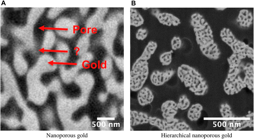
FIGURE 1. Back-scattered electron scanning microscope images of epoxy-infiltrated nanoporous gold (npg) and hierarchical nanoporous gold (hnpg). (A) nanoporous gold structures below the cross-section plane shine through the epoxy-filled pores so that for some pixels it is unclear whether they belong to the solid (gold) or the pore (epoxy) phase (arrow with the question mark). (B) The influence of the shine-through effect is increased in hierarchical nanoporous gold due to the small pore sizes within the ligaments.

Classical methods like thresholding work best for standard materials without nanopores (Salzer et al., 2015). However, they fail for nanoporous materials with strong shine-through effects because of the ambiguity in the local voxel intensity. Machine learning algorithms like random forests or the k-means algorithm can help classify material and pores (Rogge and Ritter, 2018; Fager et al., 2020). However, deep learning-based (DL) methods, especially convolutional neural networks (CNN), bear the potential to outperform such methods when processing images. Over the last years, CNNs have more and more outperformed such classical methods across all disciplines (Krizhevsky et al., 2012; Girshick et al., 2014). For example, CNNs were used for the semantic segmentation of electron microscopy images of neuronal membranes (Ciresan et al., 2012). For the segmentation of FIB tomography images of porous membranes, the deep learning architecture ResUNet was applied, using initial training data generated by a random forest algorithm (Tracey et al., 2019). It is thus consequential to apply convolutional neural networks like U-Net, which was originally developed for biomedical images (Ronneberger et al., 2015), with some modifications also to FIB tomography data (Fend et al., 2021).

Due to shine-through effects in FIB tomography datasets, structures are visible through several subsequent SEM slices. Taking this information into account is an important step towards accurate segmentation of FIB tomography data of nanoporous materials. The machine learning architecture called CNN 2.5D has recently been reported to be particularly powerful (Vu et al., 2020) to incorporate such partial spatial information in a specific direction. CNN 2.5D feeds several adjacent slices into channels of a 2D CNN architecture. A similar approach, but with 3D kernels, is pursued by two other recently proposed machine learning architectures, 3D U-Net (Çiçek et al., 2016), and VNet (Milletari et al., 2016). The latter seeks to prevent information loss when the network grows deeper (Milletari et al., 2016).

Deep learning requires, however, a large amount of training data. In the context of the semantic segmentation of FIB tomography data, a sufficient amount of images is required whose pixels are labelled as belonging to specific categories (e.g., the solid or the pore phase in a nanoporous material). Obtaining sufficient training data from experiments can be expensive and time-consuming. To overcome this problem, synthetic training data is frequently used (Nikolenko, 2019).

In electron microscopy, two steps are required to generate synthetic training images for deep learning segmentation methods. The first step is the generation of a realistic geometric structure. The second step is the computer simulation of the FIB tomography of this structure, i.e., synthetic back-scattered electron (BSE) imaging data.

For the first step (Fend et al., 2021), previously used geometric primitives like spheres and cylinders. However, these do not adequately resemble the microstructure of the nanoporous materials of our interest. Therefore, these are suitable only to a limited extent for generating synthetic training data for the case we are interested in.

For the second step, Monte Carlo simulations of electron microscopy imaging can be performed. These simulate the trajectories of numerous electrons, thereby providing realistic information on the appearance of SEM images of specific structures. In order to perform such simulations on very simple geometries, first programs were developed more than two decades ago and have seen continuous improvements (Lowney J, 1994; Lowney, 1995; Karabekov et al., 2003; Zhang et al., 2012; Hovington et al., 1997; Gauvin et al., 2006).

In this paper, we compare different deep learning architectures for accurately segmenting FIB tomography data of nanoporous structures despite shine-through effects. We present a novel approach to generate synthetic FIB-SEM images using Monte Carlo (MC) simulations to overcome the lack of training data for deep learning methods. To obtain as realistic synthetic training data as possible, these simulations are not performed on geometries consisting of simple geometric primitives. Instead, we compare three different ways to generate largely realistic microstructures and use the most promising of them, the so-called levelled-wave algorithm (Li et al., 2020) as a basis for our study. Using the in silico training data generated this way, we demonstrate that 2D CNN with a group of adjacent slices as input data and 3D CNN can surpass the segmentation performance of classical methods by more than 100%. In the absence of ground-truth data, we measure the segmentation performance with a novel approach, which exploits specific geometrical properties of nanoporous gold and hierarchical nanoporous gold, such as isotropy.

2 Materials and Methods

2.1 Generation of Synthetic Training Data

Synthetic FIB tomography data can be generated in two steps. The first step is the generation of virtual microstructures, and the second step is the generation of virtual SEM images of these microstructures using MC simulations.

2.1.1 Generation of Virtual Microstructures

To generate artificial microstructures that closely resemble the ones of nanoporous materials, we compared three different methods: the levelled wave method (LWM), self-similarity method (SSM) and random pore generation method (RPGM).

2.1.1.1 Levelled Wave Method

Nanoporous materials are often produced by dealloying. Theoretical analysis reveals (Li et al., 2020) that this leads to a microstructure whose geometry can be described by a superimposition of several wave vectors with an identical wavelength but different random orientations (Li et al., 2020). Subsequently, the Gaussian random field generated this way is subjected to a thresholding algorithm to divide it into a solid and a pore phase, resulting in microstructures as illustrated in Figure 2A.

FIGURE 2

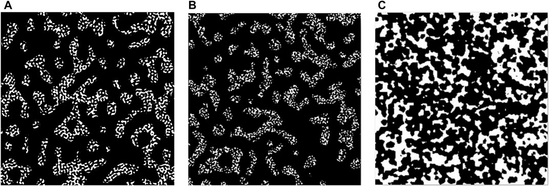
FIGURE 2. Virtual microstructures generated by (A) levelled wave method (B) self-similarity method (C) random pore generation method.

2.1.1.2 Self-Similarity Method

A structure is called self-similar if it resembles exactly or partly itself. In this method, a hierarchical microstructure is generated using the thresholded images of a real nanoporous gold structure, hence the name “self-similarity method (SSM)”. In the first step, FIB-SEM images of nanoporous gold are segmented to get binary images identifying the solid phase (intensity 255) and pore phase (intensity 0) using the k-means algorithm. Then, these binary images are resized using bilinear interpolation (Press et al., 1992) according to required voxel dimensions. In the next step, a mask, smaller in size than the binary images from the previous step, is prepared by resizing binary slices and rotating them at a random angle. Final output images are then calculated by performing arithmetic AND operations on binary images with masks using convolution (Supplementary Figure S13). These AND operations with masks generated from the original binary structure make the final structure self-similar. One slice from SSM is shown in Figure 2B.

2.1.1.3 Random Pore Generation Method

RPGM is a relatively simple method. In the first step, a volume that is fully solid (intensity 255) is chosen. Subsequently, void spheres are introduced at random locations and with a radius drawn from a Gaussian random distribution using a masking operation (Supplementary Figure S14). The advantage of RPGM is that it is a straightforward method. Its disadvantage is that it produces microstructures that exhibit considerable differences compared to actual nanoporous materials, limiting their value for training accurate machine learning-based segmentation algorithms in our case. The final sample geometry generated by this method is shown in Figure 2C.

2.1.2 Monte Carlo Simulation of Electron Microscopy

The virtual microstructures generated in the above-described ways are used in Monte Carlo simulations to generate synthetic FIB tomography data. The simulation of the BSE images is performed using the software MCXray. This software is an extension of the Monte Carlo simulation tools Casino (Hovington et al., 1997) and Win X-Ray (Gauvin et al., 2006). It was developed by (Gauvin and Michaud, 2009) and then incorporated in the Dragonfly Software [ORS, Montreal, Canada] (Object Research Systems, 2018). MCXray allows simulations of complex microstructures even consisting of different materials. Simulated BSE images of virtual microstructures generated by the above described three methods are presented in Figure 3. In all the Monte Carlo simulations for this paper, we assume beam energy of 2 kV, a beam current of 5 × 10^–11 A, FIB sample stage tilt angle of 0 degrees, and detector to sample distance of 104 mm. We performed these simulations for nanoporous gold and hierarchical nanoporous gold, and considered pores in vacuum (Figure 3) as well as infiltrated with epoxy resin (see for example Figures 4–B). These simulations have a high shine-through effect and mimic images from a less surface sensitive through-the-lens (TLD) back-scattered electron detector.

FIGURE 3

FIGURE 3. Simulated BSE images using Monte Carlo simulation method and data generated using (A) LWM as initial virtual structure (B) SSM as initial virtual structure (C) RPGM as initial virtual structure.

FIGURE 4

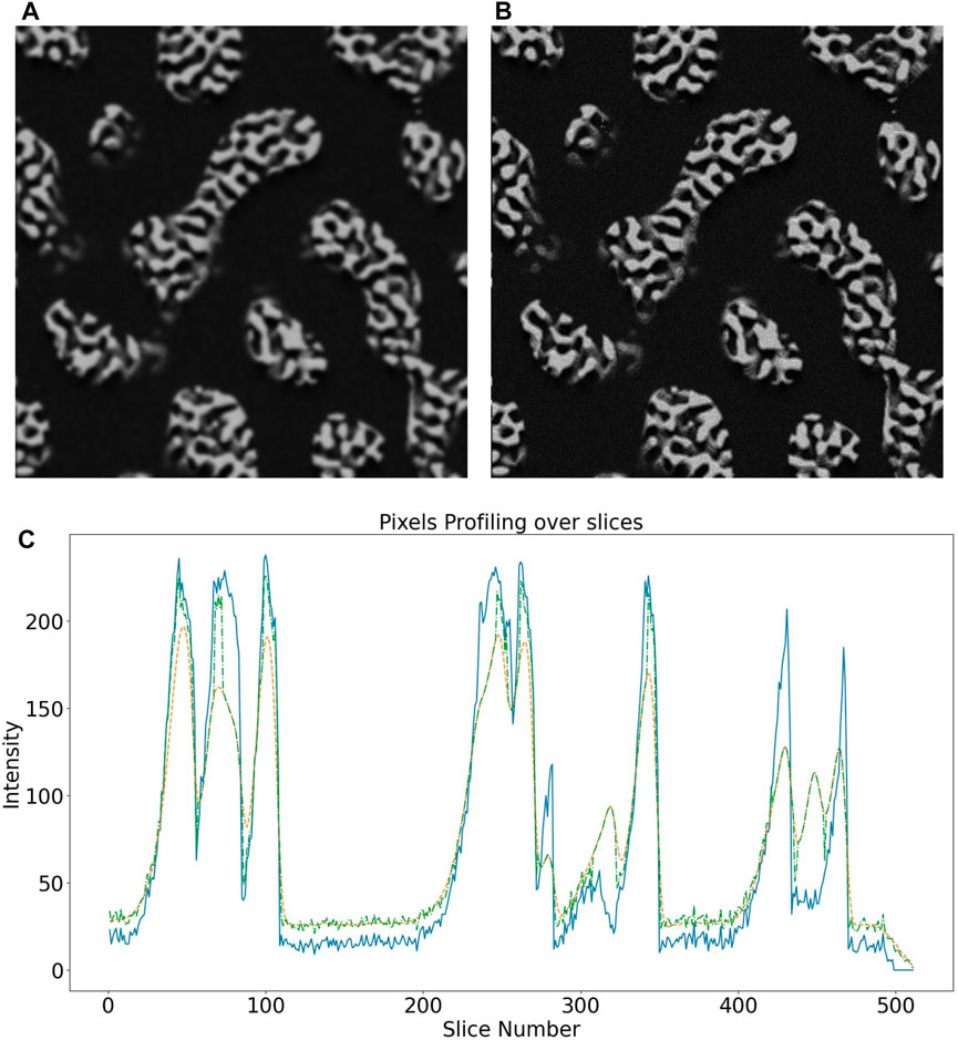
FIGURE 4. Synthetic SEM image after applying (A) standard Gaussian blur filter and (B) the 4-step blurring procedure introduced herein (C) intensities of pixel located at a random location in the xy-plane across slices before blurring (blue), after applying Gaussian blur filter (orange) and 4-step blurring procedure (green).

2.2 Preprocessing of Training Data

In our study, we applied noise and blur filters to make the simulated images more similar to actual FIB tomography data. Subsequently, we applied the online data augmentation technique to increase the size of the training dataset.

2.2.1 Adding Noise

Electron microscopy images typically exhibit two types of noise (Cizmar et al., 2008). Primary electrons can generate Poisson noise, and the rest of the electrons from five noise sources can generate Gaussian noise (Timischl et al., 2012). Not all five sources are equally important, and noise added by detection systems is often assumed to be negligible (Sim et al., 2004; Goldstein, 2003). MCXray (Gauvin and Michaud, 2009) simulations of BSE images naturally include Gaussian noise (Hovington et al., 1997). We added the remaining Poisson noise and some additional Gaussian noise to understand the effect of noise in synthetic SEM images. To this end, we used the Scikit image library¹ in this project. First, Poisson noise was added to the image, and then Gaussian noise, to get a realistic noisy simulated BSE image. For the Gaussian noise, we heuristically chose a zero mean value and a variance of 0.001. After adding the noise, the intensities of the image were renormalized to a range from -1 to 1, converting the noisy image thereby to a standard unsigned 8-bit image. As training data for our study, we used these resulting noisy images.

2.2.2 Blurring of Edges

In the images generated by MCXray simulations², the edges were observed to be unrealistically sharp. Simple solutions like applying Gaussian filtering to the whole image may not work as it may remove necessary Gaussian randomness of intensities from the solid ligaments in the simulated image. Therefore, it is very important to blur only the edges of the ligaments. This can be achieved by the following steps of masking and blurring.

1. Find edges of the solid ligaments

2. Generate mask with maximum weights at the edges from step (1)

3. Blur whole original image

4. Blend source image and blurred image from step (3) by mask from step (2)

The difference between this procedure and standard Gaussian blurring is illustrated in Figure 4. The image generated by the above 4-step procedure looks more realistic.

2.2.3 Data Augmentation

Data augmentation is a very powerful technique in deep learning when there is not enough training data available (Wang et al., 2017). Herein, we used online data upsampling; during the training process itself, the training data was augmented by applying random flips, rotations, brightness changes, and stretch transforms.

2.3 Machine Learning Architectures for Segmentation

In our synthetic FIB tomography data - as in real data - shine-through effects occur. Hence, it can be expected that accurate segmentation is not possible by processing image data layer by layer but rather in the group of the layers. Herein, we tested two machine learning architectures for segmentation that address this need.

2.3.1 2D CNN With Adjacent Slices

Shine-through effects establish a correlation between adjacent slices. To account for this in semantic segmentation, one has to segment different slices not separately but rather process information from several adjacent slides in each segmentation operation. As a way to avoid computationally costly 3D convolutions, one can process information from several adjacent layers simultaneously by 2D CNN (Figure 5). To this end, we used the 2D CNN architecture U-Net (Ronneberger et al., 2015). A general limitation of this approach is that the number of slices that can be included at a time is naturally limited by the number of slices available in the 3D image stack that forms the FIB tomography data. Indeed this limits the depth to which segmentation can be performed.

FIGURE 5

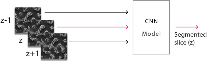
FIGURE 5. Basic block diagram of 2D CNN receiving as input for the segmentation of slice z also the slices z − 1 (above) and z + 1 (below).

2.3.2 3D CNN

While 2D CNNs are computationally cheaper than 3D CNN, they may always be prone to miss out on recognizing some spatial features. To overcome this problem, we also tested 3D CNN. These use full 3D convolutions. We compared the 3D CNN architectures 3D U-Net (Çiçek et al., 2016), VNet (Milletari et al., 2016) and ResUNet3D with minor modifications. In the U-Net architecture (Ronneberger et al., 2015) we used padding in the convolutional blocks to retain the original image size. Moreover, we also added residual connections in one of our 3D U-Net models. We considered the number of encoding blocks as a hyperparameter and tuned it to improve performance.

2.4 Training of Neural Networks

All machine learning architectures were implemented using PyTorch; data loaders were written in Python, and models were trained on Tesla K80 GPUs.

2.4.1 2D CNN With Adjacent Slices

Input to the deep neural network was provided using the sliding window technique (Figure 6), where small patches (64 × 64 pixels) were generated from the original training dataset and used as the final training set for the network. We used 3, 5, 7 and 9 slices as the number of adjacent slices, making the input window size 64 × 64 × 3, 5, 7 and 9, to understand the effect of the number of adjacent slices on the segmentation performance. Additional parameters used for the training process are specified in Table 1.

FIGURE 6

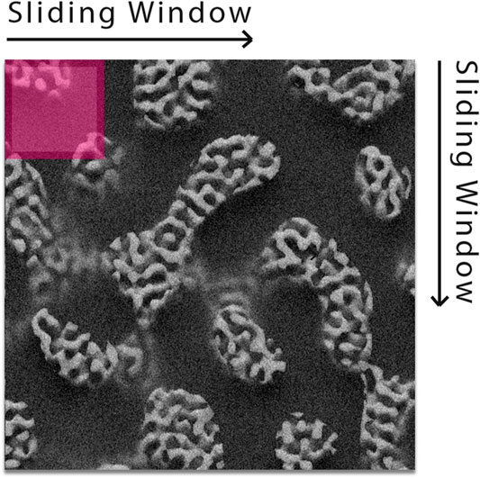
FIGURE 6. Sliding window method.

TABLE 1

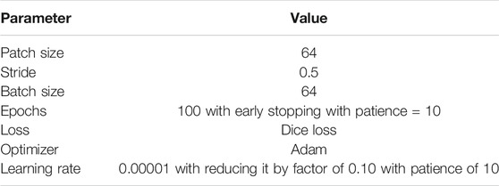
TABLE 1. Parameters used for training 2D CNN with adjacent slices.

2.4.2 3D CNN

We trained and compared a total of three 3D CNN models, namely U-Net3D, ResUNet and VNet. We used the same sliding window technique for all of them. However, unlike for the 2D CNN, the window was moving in all three spatial directions with a given stride. The training parameters are summarized in Table 2. Inspired by (Milletari et al., 2016), we used a squared Dice loss layer with the necessary smoothness value to avoid zero division in all three 3D CNN architectures. We used the mean Dice loss as the final loss value to account for possible data imbalance (Milletari et al., 2016).

TABLE 2

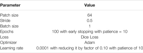
TABLE 2. Parameters used for training 3D CNN.

2.5 Evaluation Criteria

Due to the unavailability of labelled datasets, the CNN models were trained based on synthetic training and validation data. Moreover, to evaluate the performance of various segmentation methods for real BSE images, we used the concept of anisotropy (Supplementary Section S1). The shine-through effect makes the images anisotropic in the z-direction (though the underlying material microstructure is in a statistical sense isotropic, that is, lacking any preferred direction). Therefore, if the segmented images are isotropic, then it can be concluded that the segmentation method has (likely) been able to filter the shine-through effect and performs well. To measure anisotropy of the segmented images, we used two-point correlation functions (TPCF), Supplementary Figures S7, S8, and lineal path functions (LPF) for segmented ICD images (Supplementary Figures S10, S11) using our method and Otsu’s thresholding method. This set of real imaging data, referred to henceforth as hnpg_epoxy dataset, has a voxel size of 2.6 × 2.6 × 10 nm³, which was interpolated to 5.2 × 5.2 × 5.2 nm³ using bicubic interpolation. To quantify anisotropy of the segmented images, we calculated the TPCF and LPF in the x-, y- and z-direction. Subsequently, we computed the relative L2 differences for the TPCF and LPF in z-direction and compared them to the relative L2 differences for the TPCF and LPF in x- and y-direction, respectively. Generally, the relative L2 difference between two functions f and g can be computed in a discrete setting with n given data points as

$e_{L2}\left(f,g\right)=\frac{2\times \sqrt{{\sum }_{i=1}^n{\left(f_i-g_i\right)}^2}}{\left(\sqrt{{\sum }_{i=1}^n{\left(f_i\right)}^2}+\sqrt{{\sum }_{i=1}^n{\left(g_i\right)}^2}\right)}(1)$

where the f_i, g_i with i = 1, … , n are the given data points. Finally, we averaged the L2 differences of the z-direction compared to the x- and y-direction. This average is referred to henceforth (e.g., in Table 4) as TPCF or LPF e_L2 difference. The larger both are, the higher the anisotropy of the segmented images, which can be considered a hint that the associated segmentation method has not been able to filter shine-through effects.

As an additional measure of anisotropy, we calculated the average diameters of ligaments in xy-, yz- and xz-planes using lineal path functions (D_xy, D_yz, D_xz). Then, we computed the averaged relative difference $e_{D_{L2}}$ of the diameters in the xz- and yz-planes compared to the one in the xy-plane as

$e_{D_{L2}}=\frac{1}{2}\left(\sqrt{\frac{{\left(D_{xz}-D_{xy}\right)}^2}{D_{xy}^2}}+\sqrt{\frac{{\left(D_{yz}-D_{xy}\right)}^2}{D_{xy}^2}}\right)(2)$

Generally, the average diameter of ligaments in the z-direction is expected to be larger than in the x- and y-direction in the presence of non-filtered shine-through effects. Therefore, pronounced shine-through effects can be expected to result in large $e_{D_{L2}}$.

In the absence of ground truth, we also checked the congruency between images from two different sensors. We segmented FIB-SEM images from a low-loss in-column back-scattered electron detector (ICD) and compared the results with segmented images from the TLD. The ICD detector is situated at an upper position in the column, ensuring that only the most elastically scattered electrons (i.e., back-scattered electrons) are collected. The signal is highly sensitive to Z-contrast with almost no topographical information. Also, low energy loss increases the probability of near-surface interaction and therefore near-surface information (Ritter, 2019) (Figures 7–B). Therefore, one can expect the ICD images to have relatively small shine-through effects anyway so that they can provide at least some hint at the (not exactly known) ground truth. We calculated the fraction of misplaced pixels by

$MP=\frac{\left(TP-IP\right)}{TP}\times 100(3)$

where TP is the total number of pixels, IP the number of pixels identically segmented for TLD and ICD images, and MP is the fraction of pixels where the segmentation of TLD and associated ICD images disagreed.

FIGURE 7

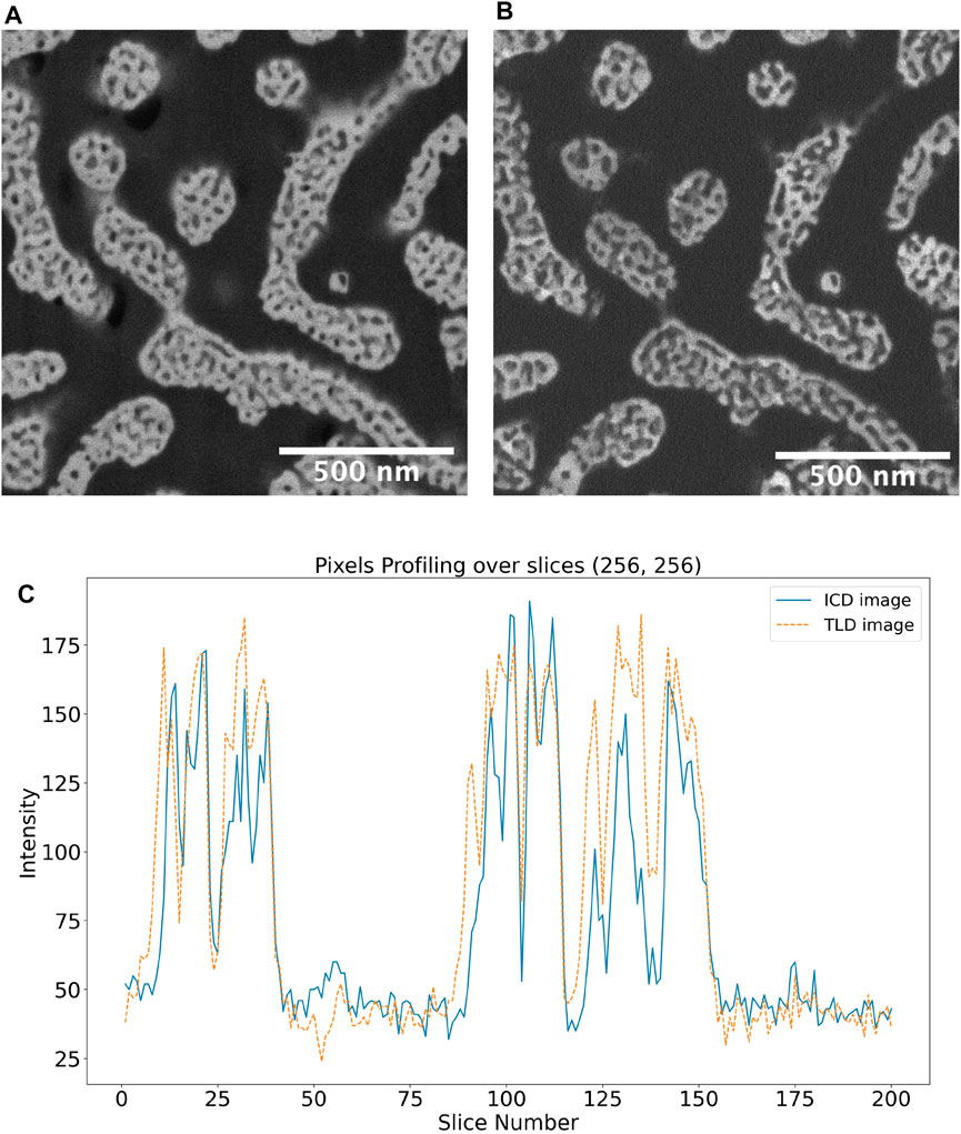
FIGURE 7. SEM images of hierarchical nanoporous gold simultaneously recorded with (A) TLD and (B) ICD detector (C) intensities of pixel located at a random location in the xy-plane in SEM TLD (orange) and ICD (orange) images.

3 Results and Discussion

3.1 Selection of Best Synthetic Training Data

The first question we sought to address was which of the three above described methods of generating synthetic training data (LWM, SSM, RPGM) is most suitable for training deep neural networks for semantic segmentation. We performed a study using the CNN architecture U-Net to answer this question. We trained the U-Net on the above three types of synthetic data, splitting them into training data (60%), validation data (20%), and test data (20%). Subsequently, we compared the performance of the trained U-Nets to two classical segmentation methods, Otsu’s thresholding algorithm (Otsu, 1979) and k-means clustering (Lloyd, 1982) with k = 3.

To evaluate the performance of these segmentation methods, we generated a synthetic dataset called npg40, which was prepared using MC simulations on synthetic microstructures generated by k-means segmentation of real nanoporous gold SEM images. The performance of the models was then evaluated using metrics as the relative error of solid volume fraction and the Dice coefficients. As shown in Table 3, the deep learning model trained on the LWM data exhibits the lowest solid volume fraction error and highest Dice coefficient. Therefore, we trained all our deep learning models, shown below, using synthetic LWM data only after this preliminary test.

TABLE 3

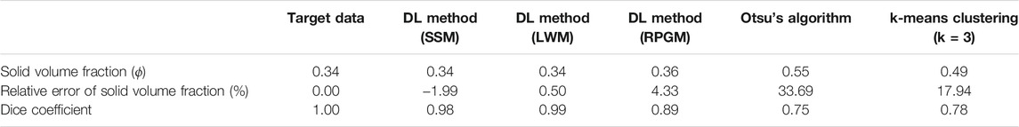
TABLE 3. Performance of different segmentation methods applied to dataset npg40.

3.2 Role of Preprocessing

It is instructive to compare the performance of segmentation methods trained on synthetic training data with and without preprocessing (“blur the edges” and subsequent addition of noise). To this end, we trained 3D CNN and 2D CNN processing adjacent slices (on synthetic LWM data) and subsequently compared their segmentation performance on the (real) hnpg_epoxy dataset. Table 4 reveals that preprocessing increases segmentation performance for both 2D CNN processing adjacent slices and 3D CNN, underlining that preprocessing indeed helps to generate more realistic synthetic training data.

TABLE 4

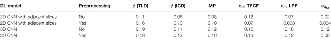
TABLE 4. Impact of preprocessing on segmentation performance for real hnpg_epoxy dataset.

3.3 Semantic Segmentation

We validated our trained models and their performance both by the segmentation of one synthetic LWM dataset and four sets of real FIB-SEM images (see Table 5). Results are presented in Tables 6, 7, and 8. In these tables, it is apparent that the L2 differences for the TPCF and LPF and also the ligament diameter anisotropy is much lower for the novel segmentation methods based on deep learning introduced in this paper compared to classical methods like Otsu’s method or k-means clustering (with k = 3). This suggests that our novel deep learning methods filter shine-through effects much better than classical methods and thus produce a geometry much closer to the real one. The excessive solid volume fraction of the segmented ICD data compared to the associated TLD data suggests that, in particular, Otsu’s thresholding method in many cases fails to classify pixels visible due to the shine-through effect. Our deep learning-based segmentation methods exhibit much lower MP values compared to Otsu’s method and k-means clustering. That is, they succeed in more cases to classify pixels in TLD and ICD imaging data identically. Following the concept of sensor fusion, also this is indicative of a better performance of our deep learning-based segmentation methods. It is interesting to discuss why there is a particularly large number of misplaced pixels for both real data sets when using k-means clustering. To explain this, it is important to note that we selected k = 3 for k-means clustering to account for the presence of a total of three different clusters, namely a solid phase, a pore phase and artifacts (i.e. pixels due to the shine-through effect). This assumption is certainly reasonable for TLD images because of their sensitivity to shine-through effects. By contrast, ICD images are much less prone to this problem, so k = 3 may no longer be a good assumption, resulting in poor performance of the associated segmentation.

TABLE 5

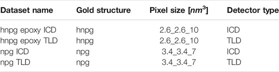
TABLE 5. Specifications of real FIB-SEM gold datasets used in this study. Note: All dataset discussed in the table have epoxy material as pore filling.

TABLE 6

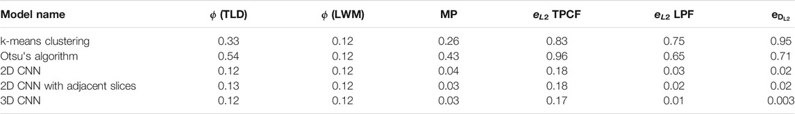
TABLE 6. Performance of different segmentation methods applied to synthetic LWM dataset. MP is here computed not using ICD images as reference but exact synthetic microstructure generated by the LWM.

TABLE 7

TABLE 7. Performance of different segmentation methods applied to real hnpg_epoxy_TLD dataset.

TABLE 8

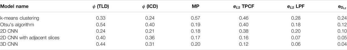
TABLE 8. Performance of different segmentation methods applied to real npg_TLD dataset.

Among the CNN-based segmentation methods, the 2D CNN with adjacent slices and the 3D CNN performed better than the standard 2D CNN. They probably can generalize better to the different datasets. For example, the very low solid volume fraction in Table 8 for the 2D CNN segmentation suggests that this method fails to classify solid pixels for the npg_TLD dataset.

We also studied the effects of window size (number of adjacent slices) on segmentation performance. It is evident from Figure 8 that 2D CNN processing adjacent slices provided the best performance for windows of sizes 9 and 5 for the hnpg_epoxy_TLD and the npg_TLD datasets, respectively.

FIGURE 8

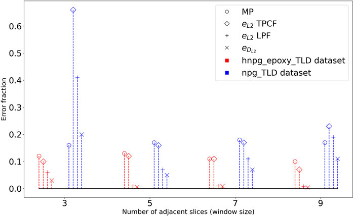
FIGURE 8. Effect of window size when using 2D CNNs with adjacent slices for segmentation for the real datasets from Table 5.

4 Conclusion

Deep learning can play an important role in the segmentation of FIB tomography data. A potential caveat is the limited availability of training data. We demonstrated that the lack of training data can be overcome by generating virtual microstructures and simulating them using the MCXray method, providing ample synthetic FIB tomography training data. We compared three different methods to generate realistic synthetic nanoporous geometries. Our results reveal that the training data generated by the levelled wave method (LWM) is most effective for deep learning of image segmentation. A major problem in this context is the typically missing availability of ground truth. That is, for real materials, most often, there is no information available that would characterize their microstructure more accurately and reliably than segmented FIB tomography data, which makes it naturally difficult to evaluate the performance of a specific segmentation method. Herein, we introduced a novel approach to measure the extent to which shine-through effects - which can be expected to be the dominant source of errors in the semantic segmentation of images of nanoporous materials - are filtered out by different segmentation methods. This method did not require any full ground truth but rather exploited that nanoporous materials typically exhibit an isotropic microstructure. This way, the degree of anisotropy of the segmented images could be used as a proxy of the segmentation error. We tested different deep learning architectures for the segmentation of FIB tomography data and identified 2D CNNs with adjacent slices as image channels and 3D CNNs as the best architectures of the ones tested herein. Generally, 3D CNNs were found to be computationally more expensive to train than 2D CNN with adjacent slices.

Data Availability Statement

The datasets generated and analyzed for this study can be found in TUHH Open Research repository (https://tore.tuhh.de/handle/11420/11060).

Author Contributions

TS, RA, CC, and MR contributed to conception and design of the study. YL generated the LWM database. NP and RG helped with the formation of Monte Carlo simulations. TS wrote the first draft of the manuscript. All authors contributed to manuscript revision, read, and approved the submitted version.

Funding

This work was funded by the Deutsche Forschungsgemeinschaft (DFG, German Research Foundation) – SFB 986 – Project number 192 346 071.

Conflict of Interest

The authors declare that the research was conducted in the absence of any commercial or financial relationships that could be construed as a potential conflict of interest.

Publisher’s Note

All claims expressed in this article are solely those of the authors and do not necessarily represent those of their affiliated organizations, or those of the publisher, the editors and the reviewers. Any product that may be evaluated in this article, or claim that may be made by its manufacturer, is not guaranteed or endorsed by the publisher.

Acknowledgments

We thank Stefan Bartels for his contribution by providing us the necessary computation power to generate the simulated images in this study.

Supplementary Material

The Supplementary Material for this article can be found online at: https://www.frontiersin.org/articles/10.3389/fmats.2022.837006/full#supplementary-material

Footnotes

¹https://scikit-image.org

²Dragonfly software version 2021.1.0.118 13. Blurring of edges may not require in future versions of the software

References

Ciresan, D., Giusti, A., Gambardella, L., and Schmidhuber, J. (2012). Deep Neural Networks Segment Neuronal Membranes in Electron Microscopy Images. Adv. Neural Inf. Process. Syst. 25, 2843–2851.

Google Scholar

Cizmar, P., Vladár, A. E., Ming, B., and Postek, M. T. (2008). For the National Institute of Standards and TechnologySimulated Sem Images for Resolution Measurement. Scanning 30, 381–391. doi:10.1002/sca.20120

PubMed Abstract | CrossRef Full Text | Google Scholar

Çiçek, Ö., Abdulkadir, A., Lienkamp, S. S., Brox, T., and Ronneberger, O. (2016). “3d U-Net: Learning Dense Volumetric Segmentation from Sparse Annotation,” in International conference on medical image computing and computer-assisted intervention (Berlin, Germany: Springer), 424–432. doi:10.1007/978-3-319-46723-8_49

CrossRef Full Text | Google Scholar

Fager, C., Röding, M., Olsson, A., Lorén, N., von Corswant, C., Särkkä, A., et al. (2020). Optimization of FIB-SEM Tomography and Reconstruction for Soft, Porous, and Poorly Conducting Materials. Microsc. Microanal 26, 837–845. doi:10.1017/s1431927620001592

PubMed Abstract | CrossRef Full Text | Google Scholar

Fend, C., Moghiseh, A., Redenbach, C., and Schladitz, K. (2021). Reconstruction of Highly Porous Structures from FIB‐SEM Using a Deep Neural Network Trained on Synthetic Images. J. Microsc. 281, 16–27. doi:10.1111/jmi.12944

CrossRef Full Text | Google Scholar

Gauvin, R., Lifshin, E., Demers, H., Horny, P., and Campbell, H. (2006). Win x-ray: A New Monte Carlo Program that Computes X-ray Spectra Obtained with a Scanning Electron Microscope. Microsc. Microanal. 12, 49–64. doi:10.1017/s1431927606060089

PubMed Abstract | CrossRef Full Text | Google Scholar

Gauvin, R., and Michaud, P. (2009). Mc x-ray, a New Monte Carlo Program for Quantitative X-ray Microanalysis of Real Materials. Microsc. Microanal 15, 488–489. doi:10.1017/s1431927609092423

CrossRef Full Text | Google Scholar

Girshick, R., Donahue, J., Darrell, T., and Malik, J. (2014). “Rich Feature Hierarchies for Accurate Object Detection and Semantic Segmentation,” in Proceedings of the IEEE conference on computer vision and pattern recognition, 580–587. doi:10.1109/cvpr.2014.81

CrossRef Full Text | Google Scholar

Goldstein, J. (2003). Scanning Electron Microscopy and X-Ray Microanalysis. Berlin, Germany: Springer US.

Google Scholar

Hovington, P., Drouin, D., and Gauvin, R. (1997). Casino: A New Monte Carlo Code in C Language for Electron Beam Interaction—Part I: Description of the Program. Scanning 19, 1–14. doi:10.1002/sca.4950190104

CrossRef Full Text | Google Scholar

Karabekov, A., Zoran, O., Rosenberg, Z., and Eytan, G. (2003). Using Monte Carlo Simulation for Accurate Critical Dimension Metrology of Super Small Isolated Poly-Lines. Scanning: J. Scanning Microscopies 25, 291–296.

Google Scholar

Knott, G., Marchman, H., Wall, D., and Lich, B. (2008). Serial Section Scanning Electron Microscopy of Adult Brain Tissue Using Focused Ion Beam Milling. J. Neurosci. 28, 2959–2964. doi:10.1523/jneurosci.3189-07.2008

CrossRef Full Text | Google Scholar

Krizhevsky, A., Sutskever, I., and Hinton, G. E. (2017). Imagenet Classification with Deep Convolutional Neural Networks. Commun. ACM 60, 84–90. doi:10.1145/3065386

CrossRef Full Text | Google Scholar

Li, Y., Dinh Ngô, B.-N., Markmann, J., and Weissmüller, J. (2020). Datasets for the Microstructure of Nanoscale Metal Network Structures and for its Evolution during Coarsening. Data in brief 29, 105030. doi:10.1016/j.dib.2019.105030

PubMed Abstract | CrossRef Full Text | Google Scholar

Lloyd, S. (1982). Least Squares Quantization in Pcm. IEEE Trans. Inform. Theor. 28, 129–137. doi:10.1109/tit.1982.1056489

CrossRef Full Text | Google Scholar

Lowney J, M. E. (1994). User’s Manual for the Program Monsel-1: Monte Carlo Simulation of Sem Signals for Linewidth Metrology. Gaithersburg, Maryland, U.S.: NIST special publication.

Google Scholar

Lowney, J. (1995). Monsel-ii Monte Carlo Simulation of Sem Signals for Linewidth Metrology. Gaithersburg, Maryland, U.S.: NIST special publication.

Google Scholar

Milletari, F., Navab, N., and Ahmadi, S.-A. (2016). “V-net: Fully Convolutional Neural Networks for Volumetric Medical Image Segmentation,” in 2016 fourth international conference on 3D vision (3DV) (IEEE), 565–571. doi:10.1109/3dv.2016.79

CrossRef Full Text | Google Scholar

Nikolenko, S. (2019). “Synthetic Data in Deep Learning,” in School-conference “Approximation and Data Analysis 2019”, 21.

Google Scholar

Object Research Systems (2018). Object Research Systems (ORS) Inc. Montreal, Canada: Object Research Systems (ORS) Inc. Dragonfly 3.6 [computer software].

Google Scholar

Otsu, N. (1979). A Threshold Selection Method from gray-level Histograms. IEEE Trans. Syst. Man. Cybern. 9, 62–66. doi:10.1109/tsmc.1979.4310076

CrossRef Full Text | Google Scholar

Press, W. H., Teukolsky, S. A., Flannery, B. P., and Vetterling, W. T. (1992). Numerical Recipes in Fortran 77: Volume 1, Volume 1 of Fortran Numerical Recipes: The Art of Scientific Computing. Cambridge: Cambridge University Press.

Google Scholar

Prill, T., Schladitz, K., Jeulin, D., Faessel, M., and Wieser, C. (2013). Morphological Segmentation of Fib-Sem Data of Highly Porous media. J. Microsc. 250, 77–87. doi:10.1111/jmi.12021

CrossRef Full Text | Google Scholar

Ritter, M. (2019). Comparison of 3d-Fib Tomography Volume Reconstruction with Various In-Column Detectors on an Epoxy-Infiltrated Nonoporous Metal Test Sample,” in EMAS 2019—16th European Workshop on Modern Developments and Applications in Microbeam Analysis.

Google Scholar

Rogge, F., and Ritter, M. (2018). Cluster Analysis for Fib Tomography of Nanoporous Materials,” in EMAS 2019—19th International Microscopy Congress (IMC19).

Google Scholar

Ronneberger, O., Fischer, P., and Brox, T. (2015). “U-net: Convolutional Networks for Biomedical Image Segmentation,” in International Conference on Medical image computing and computer-assisted intervention (Berlin, Germany: Springer), 234–241. doi:10.1007/978-3-319-24574-4_28

CrossRef Full Text | Google Scholar

Salzer, M., Prill, T., Spettl, A., Jeulin, D., Schladitz, K., and Schmidt, V. (2015). Quantitative Comparison of Segmentation Algorithms for Fib-Sem Images of Porous media. J. Microsc. 257, 23–30. doi:10.1111/jmi.12182

CrossRef Full Text | Google Scholar

Sim, K. S., Thong, J. T. L., and Phang, J. C. H. (2004). Effect of Shot Noise and Secondary Emission Noise in Scanning Electron Microscope Images. Scanning 26, 36–40. doi:10.1002/sca.4950260106

CrossRef Full Text | Google Scholar

Timischl, F., Date, M., and Nemoto, S. (2012). A Statistical Model of Signal-Noise in Scanning Electron Microscopy. Scanning 34, 137–144. doi:10.1002/sca.20282

PubMed Abstract | CrossRef Full Text | Google Scholar

Tracey, J., Lin, S. S., Jankovic, J., Zhu, A., and Zhang, S. (2019). Iterative Machine Learning Method for Pore-Back Artifact Mitigation in High Porosity Membrane Fib-Sem Image Segmentation. Microsc. Microanal 25, 186–187. doi:10.1017/s1431927619001661

CrossRef Full Text | Google Scholar

Vu, M. H., Grimbergen, G., Nyholm, T., and Löfstedt, T. (2020). Evaluation of Multislice Inputs to Convolutional Neural Networks for Medical Image Segmentation. Med. Phys. 47, 6216–6231. doi:10.1002/mp.14391

PubMed Abstract | CrossRef Full Text | Google Scholar

Wang, J., and Perez, L. (2017). The Effectiveness of Data Augmentation in Image Classification Using Deep Learning. Convolutional Neural Networks Vis. Recognit 11, 1–8.

Google Scholar

Zhang, P., Wang, H. Y., Li, Y. G., Mao, S. F., and Ding, Z. J. (2012). Monte Carlo Simulation of Secondary Electron Images for Real Sample Structures in Scanning Electron Microscopy. Scanning 34, 145–150. doi:10.1002/sca.20288

PubMed Abstract | CrossRef Full Text | Google Scholar