Emulating quantum dynamics with neural networks via knowledge distillation

We introduce an efficient training framework for constructing machine learning-based emulators and demonstrate its capability by training an artificial neural network to predict the time evolution of quantum wave packets propagating through a potential landscape. This approach is based on the idea of knowledge distillation and uses elements of curriculum learning. It works by constructing a set of simple, but rich-in-physics training examples (a curriculum). These examples are used by the emulator to learn the general rules describing the time evolution of a quantum system (knowledge distillation). We show that this emulator is capable of learning the rules of quantum dynamics from a curriculum of simple training examples (wave packet interacting with a single rectangular potential barrier), and subsequently generalizes this knowledge to solve more challenging cases (propagation through an arbitrarily complex potential landscape). Furthermore, we demonstrate, that using this framework we can not only make high-fidelity predictions, but we can also learn new facts about the underlying physical system, detect symmetries, and measure relative importance of the contributing physical processes.

1 Introduction

Neural networks, with their variety of architectures Sengupta et al. (2020) have enabled novel approaches to research in domains such as physics Carleo et al. (2019), material science Schmidt et al. (2019), and quantum science Carrasquilla (2020). Many standard applications of machine learning methods can be reduced to either classification or regression tasks Alzubaidi et al. (2021). In the latter case, they have been shown to serve as powerful interpolation tools Feldman and Zhang (2020); Chai et al. (2020). However, in other scientific applications, we are more interested in extrapolation from known facts, rather than in interpolation, e.g., searching for a new material that has some unusual properties. Unfortunately, out-of-domain predictions, are typically challenging Haley and Soloway (1992); Xu et al. (2021).

The main objective of this paper is to examine the following idea: Can we train a neural network using some easily generated—but rich in physics—examples, and than apply the extracted knowledge to solve some more complex cases, not represented explicitly during the training? To answer this, we propose a new training framework that promotes generalizability of neural network. Furthermore, we show how one can use neural networks to learn about the underlying physical problem, and how it can be utilized for scientific concept discovery.

Through the paper, our central focus will be on the following three aspects: knowledge extraction, generalization capability, and model interpretability. To extract knowledge, we use the concept of curriculum learning Bengio et al. (2009). Namely, we construct a training set that allows a neural network to effectively learn the basic rules governing the physics of the quantum system. This procedure can also be viewed as knowledge distillation Gou et al. (2021) from a physically-informed simulator, responsible for constructing the training examples, to an auxiliary network that learns from the prepared curriculum. This idea is rooted in the concept of teacher-network frameworks Romero et al. (2015), whereby a smaller (and simpler) machine learning model is trained to approximate a larger, more complex system. However, whereas in the original formulation, this technique was primarily used to reduce the final model complexity Hinton et al. (2015), i.e., in order to decrease the inference time and to reduce the overall computational and storage requirements, here we have another motivation. We want to promote the ability of the machine learning model to generalize (to make out-of-domain predictions). In other words, the goal here is to train on examples that are easy to construct, and then make predictions for cases that could potentially be difficult to simulate in a direct way. Finally, we want to observe how our machine learning-based emulator learns the essential physics from the physically-informed simulator. As we will show, by doing this, we can get additional insights about the nature of the underlying problem, discover symmetries, and measure the relative importance of the contributing features.

In this work, as a prove of concept, we focus on the quantum dynamics of one-dimensional systems. While the problem is fairly easy to simulate in a traditional way Figueiras et al. (2018), it also exhibits several non-trivial properties, such as wave function inference, scattering, and tunnelling. Additionally, the emulator must learn to preserve the wave function normalization and must correctly interpret the real and imaginary part of the input. Another practical advantage of this problem formulation is that we can easily scale the difficulty of the task by analyzing potential landscapes of various complexity.

The underlying motivation for focusing on quantum dynamics emulation tools is their use in simulating quantum systems and role in the design process of quantum devices, such as qubits and sensors Meyerov et al. (2020). Specifically, modeling devices that are embedded in an environment requires challenging predictions of open quantum system dynamics Candia et al. (2015); Luchnikov et al. (2019). Such simulations are inherently difficult on classical computers Loh et al. (1990); Prosen and Žnidarič (2007). The reason is that direct calculations can only be performed for fairly small systems, as the limiting factor are the exponential dimensions of their Hilbert spaces Breuer and Petruccione (2007). Consequently, new tools that offer efficient and high-fidelity approximation of quantum dynamics can help the science community to model larger and more complex systems.

1.1 Related work and novelty of our approach

Machine learning methods have recently been successfully used to solve many-electron Schrödinger equations Pfau et al. (2020); Hermann et al. (2020). However, in contrast to our work, previous focus was not on the quantum dynamics, but rather on finding equilibrium quantum states in electronic and molecular systems. Machine learning methods can be also used to solve partial differential equations (PDEs). In this context, some recent studies have been based on finite-dimensional approaches Zhu and Zabaras (2018); Bhatnagar et al. (2019), neural finite element Smith et al. (2021); Raissi et al. (2019); Raissi (2018), and Fourier neural operator methods Lu et al. (2020); Li et al. (2020). However, in most of these approaches, the trained emulators can only generalize to a specific distribution of initial conditions. Consequently, they do not generalize in the space of the PDE parameters, and therefore they need to be re-trained for each new scenario. Machine learning was also used to emulate classical fluid dynamics Sanchez-Gonzalez et al. (2020). However, in those cases the focus was placed on accelerating large-scale, classical simulations. In contrast, here we focus on quantum systems.

In the context of quantum dynamics, there has been a number of recent papers showing promise of using neural networks to predict the time evolution of wave packets, which however differ from our approach in significant ways. For example, in Secor et al. (2021), the authors predict the time evolution of wave packets for either a fixed or a specific type of slowly-evolving potential. In contrast, in our work we train the neural network to learn general rules of wave packet time evolution that are not tight to any specific potential shape. Additionally, we focus on extrapolation, whereas the cited paper is concerned with interpolation (predicting the propagation of wave packets in regimes already explored during the training).

In Lin et al. (2021), the authors use a long short-term memory (LSTM) network to predict the long-time quantum dynamics of open systems. However, they restrict the analysis only to the case of zero external potential. In contrast, we focus on propagation through arbitrarily complex potential landscapes. Additionally, we test the minimal neural network architecture required for completing our prediction tasks (e.g., we show that an recurrent-type model is not necessary when predicting propagation in absence of the external potential).

In Wu et al. (2021), the authors propose a neural network architecture capable of learning the time evolution of the reduced density matrix for a spin-boson model. The authors take long sequences of inputs (128 time-steps) and process them with the help of two layers of CNN filters before directing them to an LSTM network. While we test similar neural network architectures, there are several differences between this paper and our work. First of all, instead of solving one specific model, we concentrate here on the more general question of how to extract dynamics from a restricted set of (simple) simulations, and then how to generalize this knowledge to predict the quantum time evolution under more general circumstances. Thus, we focus on knowledge extraction, not only on forecasting. We also ask the question of what is the minimal model capable of learning quantum dynamics, in order to examine the complexity of the underlying physical problem. As we show, this approach helps us with the robustness and interpretability of the final emulator. In Rodríguez and Kananenka (2021), the authors predict long-time dynamics of open quantum systems, taking as the input values of the system reduced density matrices at discrete times. In contrast, we examine a more general case, by focusing on the propagation of wave functions in the presence of an arbitrarily complex external potential. Finally, in Choi et al. (2022), the authors present a method of learning and generating quantum trajectories of closed and open quantum systems. They achieved this by training a variational autoencoder and by modeling the dynamics of the resulting latent representation by solving an ODE equation parametrized by a separate neural network’s layer. While this approach allows extrapolating quantum trajectories (from a simple two-level quantum system to a two-qubit system), the general scope of this paper differs from our work. We do not focus on a single machine learning model that is capable of generalization, but we look at training frameworks that promote generalization for many possible neural architectures. As such, we look at the discussed work not as competing, but rather complementary to our work.

In more general terms, our training framework differs from a typical supervised setting that is often primarily concerned with in-domain predictions. We aim to extract knowledge from a curriculum of simple examples, and then generalize to more complex scenarios. Therefore our focus will be on training methods that facilitate generalization to (near) out-of-domain cases.

2 Methods

2.1 Problem formulation

We consider the one-dimensional time-dependent Schrödinger equation in atomic units,

$i\frac{\partial }{\partial t}\psi \left(x,t\right)=\mathcal{H}\psi \left(x,t\right),(1)$

where x ∈ [0, L_x), t ∈ [0, T), and the Hamiltonian operator $\mathcal{H}$ is defined as

$\mathcal{H}=T+V=-\frac{1}{2}\frac{{\partial }^2}{\partial x^2}+V\left(x\right),(2)$

with T and V being the kinetic and potential energy operators, respectively.

We represent the quantum waves as complex-valued functions, $\psi (x,t)\in \mathbb{C}$, on a N_x × N_t mesh grid, and we impose periodic boundary conditions: ψ(x + L_x, t) = ψ(x, t), where L_x is the size of our 1-dimensional environment. We use an equal mesh spacing. With Δx = L_x/N_x and Δt = T/N_t, the spatial and temporal coordinates become x_i = iΔx and t_j = jΔt, with i ∈ {0, 1, … , N_x−1} and j ∈ {0, 1, … , N_t−1}, respectively. For brevity, we denote the discrete wave function values as ${\psi }_i^j=\psi (x_i,t_j)$, and the discrete potential steps as v_i = V(x_i).

Given the discretizations described above, we consider the neural network-based emulator as a parameterized map from an input, constructed from the H consecutive time steps, {t_j, t_t+1, … , t_j+H−1}, to the output that relates to the next time step, t_j+H. To make the input and the output of the neural network independent from the size of the system, we construct a slices (we call them windows through the text) of a fixed width W. Namely, a portion of the input representing the values of the quantum wave at the time step t_j, can be written as

$\begin{array}{ll}\hfill {\mathit{\omega }}_i^j& =\left({\psi }_{i-\lfloor W/2\rfloor }^j,{\psi }_{i-\lfloor W/2\rfloor +1}^j,\dots ,{\psi }_i^j,\dots ,{\psi }_{i+\lfloor \left(W-1\right)/2\rfloor -1}^j,\right.\hfill \\ \hfill & \left.{\psi }_{i+\lfloor \left(W-1\right)/2\rfloor }^j\right).\hfill \end{array}(3)$

Similarly, a portion of the input representing the potential landscape at the same time step, can be written as

$\begin{array}{ll}\hfill {\mathit{\nu }}_i& =\left(v_{i-\lfloor W/2\rfloor },v_{i-\lfloor W/2\rfloor +1},\dots ,v_i,\dots ,v_{i+\lfloor \left(W-1\right)/2\rfloor -1},\right.\hfill \\ \hfill & \left.v_{i+\lfloor \left(W-1\right)/2\rfloor }\right).\hfill \end{array}(4)$

In Figure 1, we show how the input of raw simulation data can be decomposed into a series of windows. We use a neural network to map each input data window to an output data window. More specifically, we look for a network to learn the mapping

$f_{\mathbf{\Theta }}:\left\{{\mathit{\omega }}_i^j,{\mathit{\omega }}_i^{j+1},\dots ,{\mathit{\omega }}_i^{j+H-1},{\mathit{\nu }}_i\right\}\to \left\{{\mathit{\omega }}_i^{j+H}\right\}.(5)$

FIGURE 1

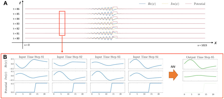
FIGURE 1. Structure of the input. (A), The input data consists of a time series of one-dimensional plots, i.e., the real and the imaginary parts of the wave function, as well as the values of the potential barrier. (B), All input information can be represented as a tensor, with three channels (similar to RGB channels when representing visual data).

Note that the dimensions of the input and the output of the neural network are different, since we have no need to predict the external potential (we assume that the potential is either static or slowly changing).

During the training, we try to find parameters Θ of the map f_Θ (represented by a neural network), that minimize the training objective function (a loss function $\mathcal{L}$) on each window output, defined as

$\mathcal{L}={\text{MSE}}_i^j=\frac{1}{W}{‖{\widehat{\mathit{\omega }}}_i^{j+H}-{\mathit{\omega }}_i^{j+H}‖}^2,(6)$

where ${\widehat{\mathit{\omega }}}_i^{j+H}$ denotes the predicted values of the quantum wave at the time step t_j in the considered window, and ${\mathit{\omega }}_i^{j+H}$ denotes the ground truth values.

2.2 Prediction using the window based scheme

To make the emulator independent of the environment size, we predict only the local evolution of the wave packet ${\mathit{\omega }}_i^j$ within a given window (cf. Figure 1B or Eq. (3)). However, to recreate the entire wave function ψ(x, t_j) for a given time step j, we need to assemble the individual predictions from different, overlapping windows. Let us denote the ${\psi }_m^j$ evaluated from window ${\mathit{\omega }}_{m+k}^j$ as ${\psi }_m^j\left({\mathit{\omega }}_{m+k}^j\right)$. We average those predictions by giving a larger weight to those predictions for which the grid-point x_m is located closer to the center of the window. For the weight, we use the Gaussian modulation,

$⟨{\psi }_m^j⟩=\sum _{k=-\lfloor \left(W-1\right)/2\rfloor }^{\lfloor W/2\rfloor }A\exp \left(-\frac{k^2}{2{\delta }^2}\right){\psi }_i^j\left({\mathit{\omega }}_{m+k}^j\right),(7)$

where $A=1/{\sum }_{k=-\lfloor (W-1)/2\rfloor }^{\lfloor W/2\rfloor }\exp \left(-k^2/2{\delta }^2\right)$ is the normalization constant, and δ denote the Gaussian averaging spread.

A complete prediction of the next time-step is a collection of all predicted points $[⟨{\psi }_0^j⟩,⟨{\psi }_1^j⟩,\dots ,⟨{\psi }_{N_x}^j⟩]$. Fortunately, all the intermediate predictions ${\psi }_m^j\left({\mathit{\omega }}_{m+k}^j\right)$ can be obtained independently, therefore the entire algorithm is easily parallelizable (e.g., by performing a batch inference on a modern GPU).

2.3 Predicting multiple steps of evolution

We predict the next time-step of the system evolution in a recurrent manner, i.e., the predictions of the previous time steps are used to form the input of the current time-step. By iteratively predicting next time-steps, we can obtain a sequence of snapshots, portraying the wave function evolution, of an arbitrary length.

2.4 Data generation and processing

Our data generation implements a two-step procedure. First, we generate raw simulation data that represents the state of the system. Then we slice them into smaller windows to feed into the neural network.

2.4.1 Raw simulation

We generate raw simulation data of wave propagation discretized on a regular mesh of size Δx = L_x/N_x, where N_x is the number of mesh points and L_x is the length of the simulation box. For the discritization, we use a space splitting method Nakano et al. (1994). Next, we simulate the wave propagation over a rectangular potential barrier of height H_b and width W_b, centered at the simulation box. Each wave funciton is parametrized by X₀, S₀, E₀, being the center-of-mass, spread, and energy of initial Gaussian-modulated wave packet, respectively. For the purpose of this work, we set L_x = 100 a. u, N_x = 1,024, and W_b = 7.0 a. u. In t = 0, the wave packet has a Gaussian modulation,

${\psi }_{t=0}\left(x\right)=C\exp \left(-\frac{{\left(x-X_0\right)}^2}{4S_0^2}\right)\exp \left(i\sqrt{2E_0}x\right).(8)$

The simulations are running with an internal-time step of Δt_int = 0.0005 a. u. We run the simulation for 100.000 steps, while saving snapshots of the simulation by every 200 steps (thus the time between each recorded, discrete time-step is Δt = 0.1 a. u). As a result, we get a tensor (N_t = 500) × (N_x = 1,024), that describes the wave function evolution. In case of a free propagation, each pixel is represented by two values, the real and the imaginary part of the wave function. In the simulations including a potential barrier, we add a third channel to each pixel, to encode values of the potential at each point.

Data windowing

To make the input of the neural network independent of the environment size, we slice the recorded raw simulation data into windows of size (H+1) × W × C. Specifically, W = 23 represents the spatial window size, C = 2 or three denotes the number of information channels, H+1 = 5 stands for the number of consequent time steps. The first H time steps are used to construct the training data set. The last time step in each simulation is used to construct the training target.

Data processing

We adopted a few techniques to efficiently process the training data. i) To reduce the correlations between training samples, we apply spatial and temporal sampling to intentionally skip some windows. We set the spatial sampling ratio to 0.1 and the temporal ratio to 0.9. ii) We assign a higher possibility to data windows overlapped with the central potential barrier. This helps us balance the “hard” and “easy” cases in the training set. iii) We apply the periodic boundary condition. iv) We renormalize the values in the channels. Specificly, the potential values are rescaled to [0, one] to improve the training stability (e.g., to mitigate the exploding gradient problem Bengio et al. (1994); Pascanu et al. (2013)).

2.5 Description of the neural network architectures

In order to find a minimum viable model, capable of solving the task, we test four different neural network architectures of increasing complexity: i) a linear model, ii) a fully-connected forward feed neural network, iii) a convolutional neural network (CNN), iv) and a recurrent neural network (using the gated recurrent units, GRU) Cho et al. (2014). More details on each architecture can be found in the Supplementary Materials.

All four models are popular choices when dealing with sequential data (cf. The models used in the papers discussed in the “Related Work” section on page §). The benefit of this approach is that we test whether the complexity of the introduced models are necessary. By choosing a simpler model we reduce the computational costs and we improve the generalizability and interpretability. Additionally, by finding the minimum viable model, we can also judge how complex the underlying physical problem is.

2.6 Training details

For the purpose of training, we generated a data set with combinations of 189 different sets of initial Gaussian wave packets and 14 different rectangular potential barriers (in total, 2,646 configurations). We kept the widths of the barrier fixed at W_b = 7 a. u. (71 pixels), the size of the environment at N_x = 1,024 pixels (with periodic boundary conditions enabled), and the window width at W = 23 pixels.

We have trained all neural networks using an AdamW optimizer Loshchilov and Hutter (2019); Kingma and Ba (2015) with a mean squared error (MSE) loss function. We selected an initial learning rate of 10^–3, with the first and second momentum being β₁ = 0.9 and β₂ = 0.99, respectively. To improve the convergence, we applied a learning rate scheduler. Namely, one percent of the total training steps were used as warm-up steps with a linearly increasing learning rate. Afterwards, the learning rate decays linearly to 10^–6. Furthermore, to improve stability of the training, we used gradient clipping as defined in Pascanu et al. (2013). More details regarding the hyper-parameters tuning are given in the Supplementary Materials.

2.7 Model evaluation

To evaluate the model’s performance, we compare the predicted evolution of the system with the ground truth, using the following two metrics: i) the mean absolute error, and ii) a normalized correlation.

We define the mean absolute error (MAE), calculated per each time step, as,

$\overline{|ϵ|}=\sum _{i=1}^{N_x}\frac{|\widehat{{\psi }_i}-{\psi }_i|}{N_x},(9)$

where N_x is the number of spatial points, while $\widehat{{\psi }_i}$ and ψ_i are the ground truth and the predicted wave function value, respectively, evaluated in the ith discrete position, x_i. MAE remains at low values for a good model. However, a consistent low MAE is not sufficient to determine a good model, as a model that constantly outputs zero or near-zero values might result in a relatively low MAE in some cases (e.g., when the ground truth is a wave packet concentrated only in a small volume of a larger space). Therefore, along the MAE, we use a secondary metric, the normalized correlation,

$\mathcal{C}=\frac{{\sum }_{i=1}^{N_x}{\widehat{{\psi }_i}}^{*}{\psi }_i}{|\widehat{\mathit{\psi }}\Vert \mathit{\psi }|},(10)$

where, N_x, $\widehat{{\psi }_i}$ and ψ_i are defined in the same way as above. The symbol * represents the complex conjugate. Normalized correlation treats the predicted and true wave functions as two vectors, i.e. $\widehat{\mathit{\psi }}$ and ψ. To this end, normalized correlation can be understood as the angular similarity between two wave function vectors.

For an overall performance evaluation, we calculate the average over a number of consequitive time steps, denoted by $⟨\overline{|ϵ|}⟩$ and $⟨\mathcal{C}⟩$ respectively.

3 Methodology

3.1 The training framework

In Figure 2, we show the proposed training framework for preparing machine learning-based quantum dynamics emulators. The main idea is based on the concepts of knowledge distillation Gou et al. (2021) and curriculum learning Bengio et al. (2009). However, instead of extracting information from a larger machine learning model, our target is a simple, physically informed simulator. In detail, the framework consists of the following steps. First, the simulator samples the initial conditions and generates time-trajectories describing an evolution of the physical system of interest (cf. Figure 2A). Next, we construct training examples from these recorded simulations (cf. Figure 2B). We select a diverse set of the training examples, making sure that all important phenomena of interest are represented (cf. Figure 2C). This balanced curriculum of examples is consequently used as the input for the machine learning model. We train the model, and then we validate it using some novel examples. When testing the model, we include cases that were not directly represented during the training, to measure whether the model can combine and generalize the acquired knowledge (cf. Figure 2D).

FIGURE 2

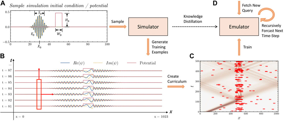
FIGURE 2. Framework for Training a Machine Learning-Based Quantum Dynamics Emulator. (A), We sample initial conditions, according to which we generate a set of physical simulations. (B), By selecting small space and time slices (illustrated by the sliding red window), we construct individual training examples. (C), We sample from the space of all possible training examples to create a training curriculum. (D), Finally, the machine learning-based emulator learns from the prepared curriculum of training examples. We test the emulator by selecting novel cases and by recursively forecasting the next time steps of the system evolution.

3.2 Training and testing procedure

To demonstrate that the emulator can extract knowledge from simple examples and generalize it in a non-trivial way, we restrict the physical simulator to cases with only a single rectangular potential barrier. The emulator need to learn from these simple examples the basic properties of the wave function propagation, namely dispersion, scattering, tunneling, and quantum wave interference. Next, we test whether the emulator can predict the time-evolution of wave packages in a more general case: e.g., for packages of different shapes propagating through an arbitrarily complex potential landscape.

To evaluate the generalization potential of the neural network-based emulators, we hand-designed a panel of test data sets that includes: random single-rectangular barriers, double-rectangular barriers, triple-rectangular barrier, irregular barriers, quadratic potentials, as well as rectangular wells.

We show these test cases in detail in Supplementary Materials.

4 Results

4.1 Quantum dynamics emulation with neural networks

We present the results of the emulation and the comparison with the ground truth in Figure 3. In panels d–e, we demonstrate the emulator’s generalizability potential on in two out-of-domain situations: with the potential barrier having a shape of a step pyramid or a smooth half-circle. Since the emulator was trained only on a single rectangular barrier of a fixed width (much wider than the width of the step in the pyramid), those testing cases can not be reduced to any examples that were seen during the training. Instead, to make valid predictions, the neural networks must recombine the acquired knowledge in a non-trivial way. Despite that challenge, as we can see in Figures 3F, G, in both cases the predictions of our emulator match well the ground truth. It is worth of noticing, that the emulator makes its predictions in a recurrent manner (by using the predictions of the previous steps as input of the next step). Therefore, it is expected that predicting the evolution over hundreds of steps will cause some error accumulation. The fact that even after 350 steps the error is negligible, speaks about the quality of the individual (step by step) predictions. This result indicates also, that long-term predictions of the dynamics are possible in our framework.

FIGURE 3

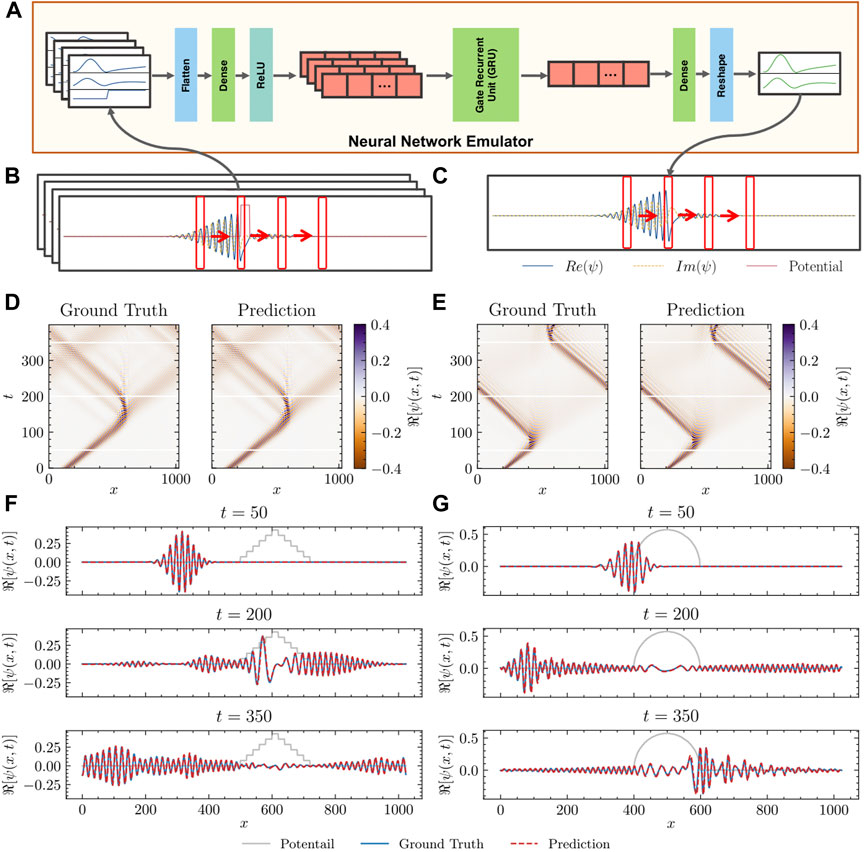
FIGURE 3. Machine Learning-Based Neural Network Emulator. (A), Proposed neural network emulator architecture, along with the corresponding input and output. The rectangle boxes illustrate different types of neural network layers, and the red arrays represent the hidden states (hidden vectors). (B), Data representation of an exemplary raw input. The red rectangles represent spatial slices of the data (windows). (C), Data representation of an exemplary output of the neural network emulator. (D), Ground truth and the predicted value of $\mathfrak{R}[\psi (x,t)]$ for an initial Gaussian wave packet and for a pyramid shaped potential barrier. (F), Comparisons of the predicted evolution and the ground truth for three temporal snapshots, t ∈{50,200,350}, depicted by the white horizontal lines in panel (D). (E,G), A similar comparison, but for a half-circle shaped potential barrier instead.

As a conclusion, the proposed neural network emulator successfully learns the classical aspects of the wave dynamics, such as dispersion and interference. It also captures the more complex quantum phenomena, such as quantum tunneling. To further show that the emulator can generalize the acquired knowledge to make both in- and out-of-distribution predictions, we hand-designed a test data set with 12 freely dispersing cases, 11 rectangular barriers (with randomly chosen width and height), as well as 14 more challenging test cases depicting both multiple and irregularly shaped barriers (in total, 37 test instances). We show a selection of those cases in Figure 4 In all cases, the results were satisfactory, confirming the ability of the emulator to generalize to novel (and notably, more challenging) situations (see also additional test results in Figs. S3 in the Supplementary Materials).

FIGURE 4

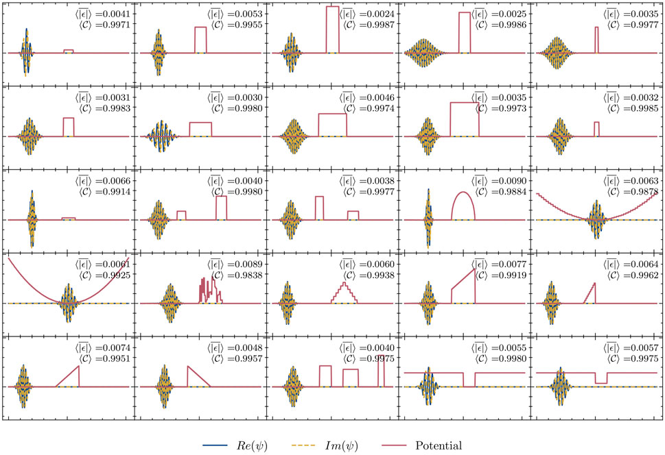
FIGURE 4. Test Cases. A selection of a hand-designed test data set for wave packet evolution in a potential landscape, along with the performance metrics of the proposed machine learning-based emulator.

4.2 Architecture justification

In this section, we aim to provide some justification for the specific architecture of the emulator, that we introduced in the previous sections. In order to verify, whether all the introduced complexity is necessary, we ask a question whether there exists a simpler machine learning model capable of learning quantum dynamics with a similar accuracy. Consequently, we compare our recurrent-network based approach with other popular network architectures. For consistency, in each case we use the same window-based scheme (to keep the input constant), while emulating the wave packet propagation for 400 time steps. When comparing with the ground truth, we measured the average mean absolute error (MAE) and the average normalized correlation $\mathcal{C}$.

The results are presented in Table 1, where the values represent the average performance over all our 37 test cases. For the comparison, we used three other models: a linear model, a densely connected feedforward model, and a convolutional model (for a detail description of each network architecture, see the Supplementary Materials). As evident in our results, the proposed architecture (utilizing the gated recurrent units, GRU) outperforms all other, simpler architectures by a large margin.

TABLE 1

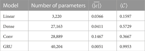
TABLE 1. Neural Network Architecture Comparison. Performance comparison for different architectures of our machine learning-based emulator. As a metric, we used the mean absolute error $\overline{|ϵ|}$ (less is better) and a normalized correlation $\mathcal{C}$ (closer to one is better), both averaged over all spatial grid points, all time step, and all available test cases.

We present a details comparison for one of our test set in Figure 5. It is evident that the recurrent architecture provides the best results, whereas the simpler architectures fail to capture the complex long-time evolution of the wave packets. Notably, a failure of each simpler model can be used to justify different aspect of our final design. For example, the failure of the linear model might indicate the importance of the non-linear activation functions included in our final model. The convolutional architecture captures quantum wave dispersion, but does not capture correctly the interaction between waves and the potential barrier. It might suggest, that to correctly capture the tunneling and scattering phenomena, we must mix the information not only between different spatial points but also between different channels. The dense architecture is able to capture both the reflection and the tunneling phenomena, but yields significant errors comparing to the recurrent-based model. This indicates, how important the temporal dimension is—something what recurrent architectures are designed to explore, as they are capable of (selectively) storing the memory of the previous steps in their internal states—and retrieving them when needed Cho et al. (2014); Gers et al. (2000).

FIGURE 5

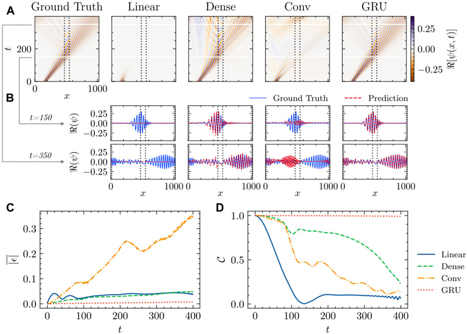
FIGURE 5. Scattering of a Quantum Wave Packet by a Rectangular Potential Barrier. (A), Ground truth and the predicted value of $\mathfrak{R}[\psi (x,t)]$ for quantum wave packets scattered by a rectangular potential barrier. (B), Comparisons of emulated and exact solutions corresponding to two temporal snapshots (time steps 150 and 350 and depicted by the white horizontal lines in panel a). (C,D), Time-step-by-time-step error propagation calculated as a mean absolute error, $\overline{|ϵ|}$ (less is better), and normalized correlations, $\mathcal{C}$ (closer to one is better), respectively.

4.3 Generalization capability

The usefulness of a neural network is mainly determined by its generalization capability. In this section, we provide a systematic analysis of both the in-domain and the out-of-domain predictive performance of our emulator.

In the training process, the raw emulation data is broken up into small windows, and those windows are re-sampled to build the curriculum. One of the reason for doing so, was to balance cases featuring different distinct phenomena, e.g., free propagation vs tunneling through the potential barrier. During the training, we artificially restricted our training instances only to those featuring Gaussian packets and single rectangular potential barriers. This allows us later to test the out-of-distribution generalizability potential—namely, whether our emulator can correctly handle packets of different modulation or barriers of complex shape.

The barrier used in our training instances had a variable height, but a fixed width of 7 a. u. Notably, the width of the window, that we used to cut chunks of the input data for our neural network, was 2.25 a. u.—i.e., it was smaller than the width of the potential barrier itself. As a result, the network was exposed during the training to three distinct situations: 1) freely dispersing quantum waves in zero potential; 2) quantum wave propagation with non-zero constant potential; 3) quantum wave propagation with a potential step from zero to a constant value of the potential (or vice versa). While it is obvious that our emulator should handle rectangular potential barriers wider than the width of the window, since such situations are analogous to those already encountered in the training process, it is not all so obvious that the same should happen with barriers of a smaller width, yet alone with barriers of different shapes than rectangular. However, as it was already presented in Figure 3, those cases do not present a challenge for our emulator.

In Figure 6, we present a more systematic study of that phenomena. We have evaluated how the accuracy of the emulation is affected when changing the following parameters: a) the initial wave packet spread, b) the initial wave packet energy, c) the rectangular barrier width, and d) the rectangular barrier height. In the experiments, we alter one of the parameters, while holding all other parameters at a constant value. We report the average correlation calculated across all the spatial grid points and all the emulated time steps. As we can see, the performance of the emulator remains effectively unchanged for all the tested values of the initial wave spread and the rectangular barrier width. This demonstrates that the network generalizes well with respect to those parameters. Remarkably, the performance does not deteriorate even when the barrier width becomes smaller than the size of the window, i.e., 2.5 a. u. This explains why our emulator was able to correctly emulate the evolution with presence of continuously-shaped barriers (that, due to the discrete nature of our input, can be seen as a collection of adjacent 1-pixel-wide rectangular barriers).

FIGURE 6

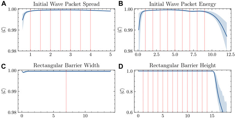
FIGURE 6. Generalization of Simulation Parameters. Average normalized correlations, denoted by $⟨\mathcal{C}⟩$, as functions of four simulation parameters: (A) initial wave packet spread, (B) initial wave packet energy, (C) rectangular barrier width, and (D) rectangular barrier height. We repeated each experiment using five different random seeds. The bold blue line in each panel shows the average normalized correlation, and the blue shades indicate the span between the minimum and maximum values recorded in those five trials. The red vertical lines denote the training values for each emulation parameter.

With respect to the value of the initial wave packet energy, the correlation curve has a “∩” shape, indicating that the accuracy deteriorates as we leave the energy-region sampled during the training stage. However, this is as much a failure to generalize as the limitation of the way how we represent the data and the environment. Lower energy of the packet means that the evolution of the quantum wave is slower—and we have to predict more steps of the simulation to cover the same spatial distance as for wave packets with a higher energy. Due to the recurrent process of our emulation, this means larger error accumulation. On the other end, when the energy is high, the wave functions change rapidly within each discretized time unit. This means a larger potential for error each time we predict the next time step. Similar situation also happens when the barrier height increases. A steeper barrier means a more dramatic changes to the values of the wave function happening between two consequent time steps. Those both effects can be mitigated by increasing either the spatial or temporal resolution of our emulation.

4.4 Model interpretability through input feature attribution

In this section, to get some insight into how our emulator makes the prediction, we measure the feature attribution (the contribution of each data input to the final prediction). We employ the direct gradient method. Namely, for a given target pixel in the output window, we calculate its gradients with respect to every input value. We follow the intuition that larger gradient is associated with higher importance of measured input Simonyan et al. (2014). Since all the target values are complex numbers, this method gives us two sets of values, one for the real and one for the imaginary value of the target pixel,

$\frac{\partial \mathfrak{R}\left({\psi }_{\text{target}}\right)}{\partial \left\{{\psi }_{\text{input}}\right\}}\text{and}\frac{\partial \mathfrak{I}\left({\psi }_{\text{target}}\right)}{\partial \left\{{\psi }_{\text{input}}\right\}}.(11)$

In Figure 7, we show a sample of the results. Namely, we selected one test example, and as the target we took the central pixel of the predicted frame. Next, we calculated the gradient with respect to each input value. In this concrete example, we can see that the importance of the input pixels increases with each consecutive time steps. However, how much exactly the early steps matter depends on the region where the predictions are made. Far from the potential barrier (cf. Figure 7A), the gradient measured with respect to the pixels of the first two steps (no. 176 and 177) is close to zero, indicating that those steps carry relative little importance. However, when predicting the evolution of the wave function in the vicinity of the potential barrier (cf. Figure 7C), the importance of the third-from-the last step (no. 177) increases noticeable. This indicates, that when predicting free propagation, the network simply performs a linear extrapolation based on the latest two time-steps. However, when predicting tunneling and scattering, the emulator reaches beyond the last two time-steps for additional information, likely due to the non-linear character of those predictions.

FIGURE 7

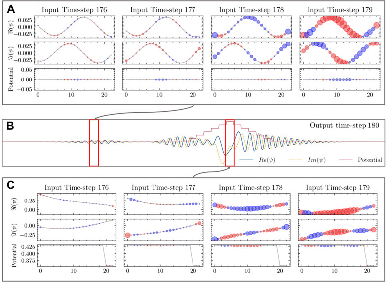
FIGURE 7. Model Interpretability. (A), Direct gradients calculated for a freely dispersing quantum wave (far from any potential barrier). Red circles denoting positive direct-gradient values, and with blue circles denoting negative values. (B), Two wave functions: one far from any potential barrier (left); second interacting with a step pyramid-shaped potential barrier (right). (C), Direct gradients calculated for a quantum wave interacting with a potential barrier.

Interestingly, when repeating the calculations for other positions of the input window, we have consistently observed similar values of the direct gradient. To further analyze this phenomenon, we measured the average value of the direct gradients for 200 randomly sampled data windows. The results are depicted in Figure 8. There is a clearly visible pattern, suggesting a steady and almost linear relationship between the input wave functions and the predicted value. This indicates, that with the absence of any potential barrier, the target values are linearly related to the input from the previous step. Introducing a potential does not change this linear mapping by much (compare the relatively small values of the standard deviation to the size of the bars). The situation is different when we consider sensitivity to the values of the potential, instead. We find that the direct gradients vary greatly over different window positions, compared to the average values. This is an indicator that the mapping from potential values to the target wave functions is a more complex, non-linear function—which is also consistent with the interpretation of the results presented earlier (cf. e.g., Figure 5 and the discussion there).

FIGURE 8

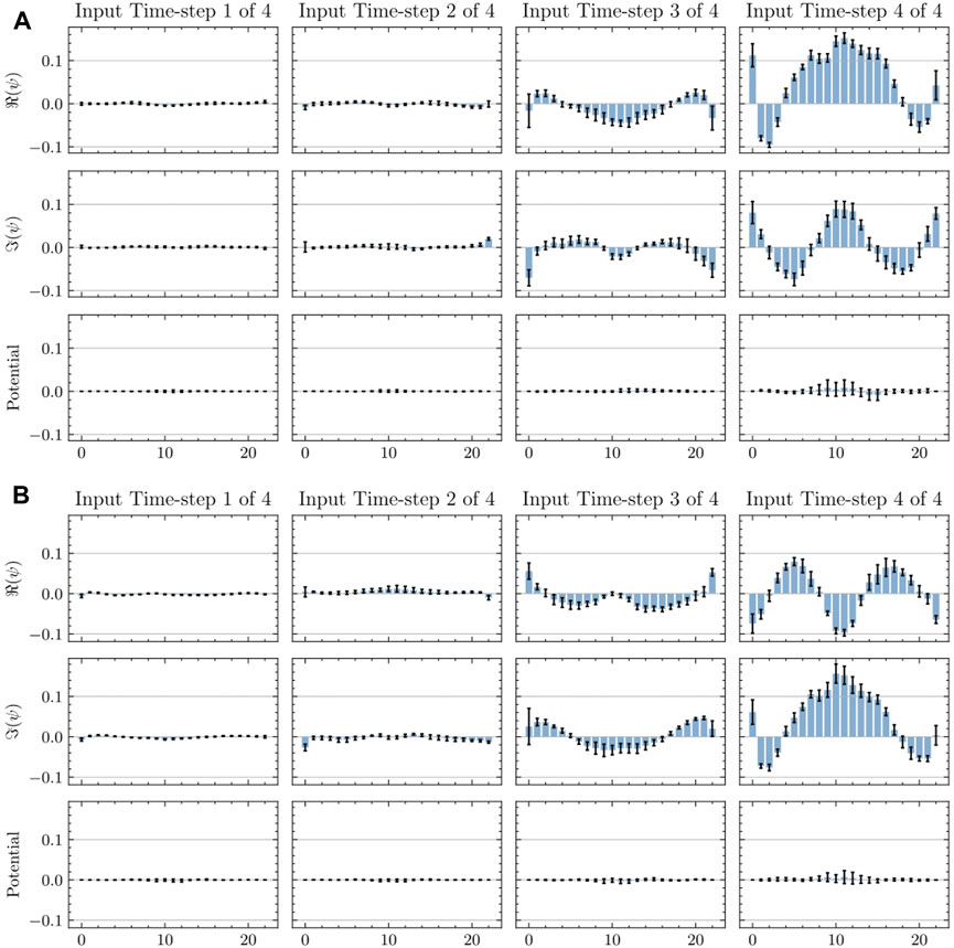
FIGURE 8. Average direct gradients. (A), The averaged direct gradients of the real part of the center pixel of the output window. (B), The averaged direct gradients of the imaginary part of the center pixel of the output window. The bars represent the average value, and the black line the standard deviation.

5 Discussion

Interpreting neural networks creates interesting possibilities. Namely, by analyzing how machine learning models make their predictions, we can learn new facts about the underlying physical problem. As an example, using the direct gradient descend method, despite its simplicity and known limitations Sundararajan et al. (2017), we can discover interesting relations between the input parameters. By analyzing several examples, such as those depicted in Figure 7, we observe a strong relationship between the averaged direct gradients of $\mathfrak{R}({\psi }_{\text{target}})$ and $\mathfrak{I}({\psi }_{\text{target}})$, namely.

$\frac{\partial \mathfrak{R}\left({\psi }_{\text{target}}\right)}{\partial \mathfrak{R}\left({\psi }_{\text{input}}\right)}=\frac{\partial \mathfrak{I}\left({\psi }_{\text{target}}\right)}{\partial \mathfrak{I}\left({\psi }_{\text{input}}\right)},\text{and}(12)$

$\frac{\partial \mathfrak{R}\left({\psi }_{\text{target}}\right)}{\partial \mathfrak{I}\left({\psi }_{\text{input}}\right)}=-\frac{\partial \mathfrak{I}\left({\psi }_{\text{target}}\right)}{\partial \mathfrak{R}\left({\psi }_{\text{input}}\right)}.(13)$

This result can be used to (re)discover the Cauchy-Riemann relations Riemann (1953). Notable, this happens, despite the fact that we have not imposed any prior knowledge of wave dynamics or complex analysis during the training procedure. rather, the model is able to learn the correct relation directly from the presented training examples.

This trend, of looking at machine learning algorithms as something more than just black-box systems capable of extracting patterns from the data or solving given classification and regression problems, opens new possibilities Zdeborová (2017, 2020). As it is evident in this example, we can use machine learning to gain a better insight into the physics problem. There has been an increasing number of papers, exploring this direction. For example, V. Bapst et al., in their article Bapst et al. (2020), demonstrated how to train a graph neural network to predict the time-evolution of a glass system. By measuring the contributions to the prediction from particles located on subsequent “shells” around the target particle, they were able to estimate the effective correlation length of the interactions. They were also able to qualitatively show, that when system approaches the glass transition, the effective cut-off distance for the particle-particle interactions increases rapidly, a phenomena that is experimentally observed in glass systems. As an another example, Lee et al., in their work Lee et al. (2022), trained support vector machines to predict the preferred phase type for the multi-principal element alloys. Next, by interpreting the trained models, they were able to discover phase-specific relations between the chemical composition of the alloys and their experimentally observed phases. Knowing what influence the phase formation, can be important both in the scientific context, as it increases our understanding, and can help us to refine our theoretical models, as well as from the manufacturing perspective, as it enables synthesis of materials with desired mechanical properties.

Another topic discussed in our paper is the ability of machine learning models to generalize to out-of-distribution examples. For the completeness, it is important to discuss what we mean by this term. We train our model on some simple examples, generated by an emulator restricted to a specific region of the parameter space. Next, we wanted to generalize in that parameter space. Namely, our goal is to predict the time-evolution of the system for parameters that are outside of the scope used during the training. This is in contrast to the typical understanding of generalization, as the ability of handling a novel (unseen during the training) data-input instances, that nevertheless come from the same distribution as the training examples. While our parameter space is relatively low-dimensional (we have just a couple of variables describing the initial conditions of the system), it is not the case for the ambient space of the inputs (each input instance is a tensor of 4 × 23 × 3, this is 276 dimensions). This high-dimensionality of the ambient space has profound implications. Balestriero, Pesenti and LeCun, in their work Balestriero et al. (2021), have shown that in highly dimensional space all predictions are effectively extrapolations, not interpolations. The logic is, that the number of training examples required for a prediction to be seen as interpolation, grows at least as fast as exponentially with the increasing dimension of the input. Effectively, for any dimensions above a few dozens, the training points become very sparse. Therefore, any point during the testing phase is likely to be far (at least along some dimensions) from any other point observed during the training. This makes that almost every testing point is located outside of the convex hull defined by the training examples—thus predictions of those points is nothing else than an extrapolation. In our case, however, we are interested in the ability to extrapolate in the space of the original parameter space, that control our physic-informed emulator, not in the ambient space of the neural network input. Since our parameters space has much lower dimension—just below 10—thus, we can distinguish cases that require interpolation and extrapolation. As an example, if our model was trained by showing propagation of wave packages with the energy spread S₀ ∈ {1, 1.5, 2, 2.5, 3, 3.5, 4}, then to predict an evolution for a package that has spread 2.7 would be an interpolation, and to predict the evolution for the spread five would be an extrapolation. In Figure 6, we have shown the performance of our emulator both in the interpolation and the extrapolation regime. We have also discussed, that the emulator can generalize outside the explored region of the parameter space, at lest along some dimensions.

There are other works discussing generalization to out-of-domain cases Wald et al. (2021); Wang et al. (2021). However, in those works the question of generalizability was asked mostly in the context of out-of-distribution detection, and used mostly in the context of fraud detection Pang et al. (2021), general novelty detection Yang et al. (2021) or as a means for increasing trustworthiness of machine learning systems Liu et al. (2020). In this paper we explored this concepts in the context of obtaining robust emulators of physical systems.

6 Conclusion

In contrast to other works that either focused on solving a specific quantum problem, e.g., prediction of long-time quantum dynamics of open systems, or on a specific class of models, e.g., the latent neural ordinary differential equation solvers, here we investigate training frameworks that promote generalization for many possible neural architectures. We also identify minimal model architectures capable of solving a given task, in order to assess the complexity of the underlying problem. And as we demonstrate, in the process of doing this, we can learn new facts about the system. This is in line with the concept of using neural networks for scientific concept discovery.

Learning from data comes at a cost. The main heavy lifting is done during the training. The training procedure can take hours, and it varies whether we train it on a CPU or a GPU. The advantage of this approach is that the inference time is constant and easily parallelizable. Nevertheless, dedicated methods tailored to emulate particular systems can be significantly faster, especially in simple cases, such as one-dimensional wave function propagation, where the overhead of the neural networks can be especially noticeable. Non-etheless, we believe that this is still acceptable, given that our neural network based approach serves different purposes, i.e., we want to learn about the system, not just solve it following a set list of instruction. To achieve this goal, we can accept some additional computational overhead.

Our framework can be applied to more than just the discussed problem. We have chosen the conceptually simple problem of one-dimensional propagation to clearly demonstrate the extent of the extrapolation capability of our approach. In this simple case, we had a wealth of controlled training data. However, this approach can be straightforwardly used on other non-linear dynamics problems with less accessible training data, such as open quantum dynamics in interacting many-body systems. In such situations our approach has the potential to provide a significant speed-up. Namely, by learning from a set of easy-to-obtain simulations, and subsequently generalizing that knowledge to more challenging cases, we can get predictions of the system’s behavior in regimes that could be hard to simulate otherwise (as long as we do not leave the regime where our predictions are still reliable - one must remember to validate the model before using it in any applications).

In future work we will optimize training schemes that maximize the generalization capability. Moreover, we will apply this methodology to physically challenging systems, e.g., including interactions. Furthermore, we will implement more sophisticated interpretability techniques and increase the robustness of the emulator by utilizing known symmetries, e.g., by constructing physically informed neural networks. Finally, we would like to pursue an iterative framework, whereby any time a new symmetry is discovered, it is implemented as a system constraint, repeating this procedure for a full characterization of the underlying physical system.

Data availability statement

The datasets presented in this study can be found in online repositories. The names of the repository/repositories and accession number(s) can be found below: https://github.com/yaoyu-33/quantum_dynamics_machine_learning.

Author contributions

The study was planned by MA and SH. The manuscript was prepared by YY, CC, SH, and MA. The data set construction was done by YY and CC. The machine learning studies were performed by both YY and CC. Result validation and code optimization was performed by MA, DK, and MA. All authors discussed the results, wrote, and commented on the manuscript.

Acknowledgments

The authors acknowledge the Center for Advanced Research Computing (CARC) at the University of Southern California for providing computing resources that have contributed to the research results reported within this publication. URL: https://carc.usc.edu. We would like to thank Prof. Oleg V. Prezhdo and Prof. Aiichiro Nakano for helpful discussions during the early stages of the project.

Conflict of interest

The authors declare that the research was conducted in the absence of any commercial or financial relationships that could be construed as a potential conflict of interest.

Publisher’s note

All claims expressed in this article are solely those of the authors and do not necessarily represent those of their affiliated organizations, or those of the publisher, the editors and the reviewers. Any product that may be evaluated in this article, or claim that may be made by its manufacturer, is not guaranteed or endorsed by the publisher.

Supplementary material

The Supplementary Material for this article can be found online at: https://www.frontiersin.org/articles/10.3389/fmats.2022.1060744/full#supplementary-material

References

Alzubaidi, L., Zhang, J., Humaidi, A. J., Al-Dujaili, A., Duan, Y., Al-Shamma, O., et al. (2021). Review of deep learning: Concepts, CNN architectures, challenges, applications, future directions. J. Big Data 8, 53. doi:10.1186/s40537-021-00444-8

PubMed Abstract | CrossRef Full Text | Google Scholar

Balestriero, R., Pesenti, J., and LeCun, Y. (2021). Learning in high dimension always amounts to extrapolation. arXiv 2110.09485.

Google Scholar

Bapst, V., Keck, T., Grabska-Barwińska, A., Donner, C., Cubuk, E. D., Schoenholz, S. S., et al. (2020). Unveiling the predictive power of static structure in glassy systems. Nat. Phys. 16, 448–454. doi:10.1038/s41567-020-0842-8

CrossRef Full Text | Google Scholar

Bengio, Y., Louradour, J., Collobert, R., and Weston, J. (2009). “Curriculum learning,” in Proceedings of the 26th Annual International Conference on Machine Learning - ICML ’09 (ACM Press). doi:10.1145/1553374.1553380

CrossRef Full Text | Google Scholar

Bengio, Y., Simard, P. Y., and Frasconi, P. (1994). Learning long-term dependencies with gradient descent is difficult. IEEE Trans. Neural Netw. 5, 157–166. doi:10.1109/72.279181

PubMed Abstract | CrossRef Full Text | Google Scholar

Bhatnagar, S., Afshar, Y., Pan, S., Duraisamy, K., and Kaushik, S. (2019). Prediction of aerodynamic flow fields using convolutional neural networks. Comput. Mech. 64, 525–545. doi:10.1007/s00466-019-01740-0

CrossRef Full Text | Google Scholar

Breuer, H.-P., and Petruccione, F. (2007). The theory of open quantum systems. Oxford University Press. doi:10.1093/acprof:oso/9780199213900.001.0001

CrossRef Full Text | Google Scholar

Candia, R. D., Pedernales, J. S., del Campo, A., Solano, E., and Casanova, J. (2015). Quantum simulation of dissipative processes without reservoir engineering. Sci. Rep. 5, 9981. doi:10.1038/srep09981

PubMed Abstract | CrossRef Full Text | Google Scholar

Carleo, G., Cirac, I., Cranmer, K., Daudet, L., Schuld, M., Tishby, N., et al. (2019). Machine learning and the physical sciences. Rev. Mod. Phys. 91, 045002. doi:10.1103/RevModPhys.91.045002

CrossRef Full Text | Google Scholar

Carrasquilla, J. (2020). Machine learning for quantum matter. Adv. Phys. X 5, 1797528. doi:10.1080/23746149.2020.1797528

CrossRef Full Text | Google Scholar

Chai, X., Gu, H., Li, F., Duan, H., Hu, X., and Lin, K. (2020). Deep learning for irregularly and regularly missing data reconstruction. Sci. Rep. 10, 3302. doi:10.1038/s41598-020-59801-x

PubMed Abstract | CrossRef Full Text | Google Scholar

Cho, K., van Merrienboer, B., Gülçehre, Ç., Bahdanau, D., Bougares, F., Schwenk, H., et al. (2014). Learning phrase representations using RNN encoder-decoder for statistical machine translation. In Proceedings of the 2014 Conference on Empirical Methods in Natural Language Processing, EMNLP 2014, October 25-29, 2014, Doha, Qatar, A meeting of SIGDAT, a Special Interest Group of the ACL, doi:10.3115/v1/d14-1179

CrossRef Full Text | Google Scholar

Choi, M., Flam-Shepherd, D., Kyaw, T. H., and Aspuru-Guzik, A. (2022). Learning quantum dynamics with latent neural ordinary differential equations. Phys. Rev. A . Coll. Park. 105, 042403. doi:10.1103/physreva.105.042403

CrossRef Full Text | Google Scholar

Feldman, V., and Zhang, C. (2020). What neural networks memorize and why: Discovering the long tail via influence estimation, 03703. arXiv 2008.

Google Scholar

Figueiras, E., Olivieri, D., Paredes, A., and Michinel, H. (2018). An open source virtual laboratory for the Schrödinger equation. Eur. J. Phys. 39, 055802. doi:10.1088/1361-6404/aac999

CrossRef Full Text | Google Scholar

Gers, F. A., Schmidhuber, J., and Cummins, F. A. (2000). Learning to forget: Continual prediction with LSTM. Neural Comput. 12, 2451–2471. doi:10.1162/089976600300015015

PubMed Abstract | CrossRef Full Text | Google Scholar

Gou, J., Yu, B., Maybank, S. J., and Tao, D. (2021). Knowledge distillation: A survey. Int. J. Comput. Vis. 129, 1789–1819. doi:10.1007/s11263-021-01453-z

CrossRef Full Text | Google Scholar

Haley, P., and Soloway, D. (1992). “Extrapolation limitations of multilayer feedforward neural networks,” in Proceedings of the IJCNN International Joint Conference on Neural Networks (IEEE). doi:10.1109/ijcnn.1992.227294

CrossRef Full Text | Google Scholar

Hermann, J., Schätzle, Z., and Noé, F. (2020). Deep-neural-network solution of the electronic Schrödinger equation. Nat. Chem. 12, 891–897. doi:10.1038/s41557-020-0544-y

PubMed Abstract | CrossRef Full Text | Google Scholar

Hinton, G., Vinyals, O., and Dean, J. (2015). “Distilling the knowledge in a neural network,” in NIPS deep learning and representation learning workshop.

Google Scholar

Kingma, D. P., and Ba, J. (2015). Adam: A method for stochastic optimization. In Proceeding of the 3rd International Conference on Learning Representations, ICLR 2015, San Diego, CA, USA.

Google Scholar

Lee, K., Ayyasamy, M. V., Delsa, P., Hartnett, T. Q., and Balachandran, P. V. (2022). Phase classification of multi-principal element alloys via interpretable machine learning. npj Comput. Mat. 8, 25. doi:10.1038/s41524-022-00704-y

CrossRef Full Text | Google Scholar

Li, Z., Kovachki, N. B., Azizzadenesheli, K., Liu, B., Bhattacharya, K., Stuart, A. M., et al. (2020). Neural operator: Graph kernel network for partial differential equations, 03485. arXiv 2003.

Google Scholar

Lin, K., Peng, J., Gu, F. L., and Lan, Z. (2021). Simulation of open quantum dynamics with bootstrap-based long short-term memory recurrent neural network. J. Phys. Chem. Lett. 12, 10225–10234. doi:10.1021/acs.jpclett.1c02672

PubMed Abstract | CrossRef Full Text | Google Scholar

Liu, W., Wang, X., Owens, J. D., and Li, Y. (2020). “Energy-based out-of-distribution detection,” in Advances in Neural Information Processing Systems 33: Annual Conference on Neural Information Processing Systems 2020, NeurIPS 2020, December 6-12, 2020, virtual.

Google Scholar

Loh, E. Y., Gubernatis, J. E., Scalettar, R. T., White, S. R., Scalapino, D. J., and Sugar, R. L. (1990). Sign problem in the numerical simulation of many-electron systems. Phys. Rev. B 41, 9301–9307. doi:10.1103/physrevb.41.9301

PubMed Abstract | CrossRef Full Text | Google Scholar

Loshchilov, I., and Hutter, F. (2019). Decoupled weight decay regularization In. Proceeding of the 7th International Conference on Learning Representations. New Orleans, LA, USA. May 6-9, 2019, (ICLR).

Google Scholar

Lu, L., Jin, P., and Karniadakis, G. E. (2020). DeepONet: Learning nonlinear operators for identifying differential equations based on the universal approximation theorem of operators. arXiv 1910.03193.

Google Scholar

Luchnikov, I., Vintskevich, S., Ouerdane, H., and Filippov, S. (2019). Simulation complexity of open quantum dynamics: Connection with tensor networks. Phys. Rev. Lett. 122, 160401. doi:10.1103/physrevlett.122.160401

PubMed Abstract | CrossRef Full Text | Google Scholar

Meyerov, I., Liniov, A., Ivanchenko, M., and Denisov, S. (2020). Simulating quantum dynamics: Evolution of algorithms in the hpc context, 04681. arXiv 2005.

Google Scholar

Nakano, A., Vashishta, P., and Kalia, R. K. (1994). Massively parallel algorithms for computational nanoelectronics based on quantum molecular dynamics. Comput. Phys. Commun. 83, 181–196. doi:10.1016/0010-4655(94)90047-7

CrossRef Full Text | Google Scholar

Pang, G., Shen, C., Cao, L., and van den Hengel, A. (2021). Deep learning for anomaly detection: A review. ACM Comput. Surv. 54, 1–38. doi:10.1145/3439950

CrossRef Full Text | Google Scholar

Pascanu, R., Mikolov, T., and Bengio, Y. (2013). “On the difficulty of training recurrent neural networks,” in Proceedings of the 30th International Conference on Machine Learning, Atlanta, GA, USA, 16-21 June 2013 (ICML 2013), 1310–1318. (JMLR.org).

Google Scholar

Pfau, D., Spencer, J. S., Matthews, A. G. D. G., and Foulkes, W. M. C. (2020). Ab initio solution of the many-electron Schrödinger equation with deep neural networks. Phys. Rev. Res. 2, 033429. doi:10.1103/physrevresearch.2.033429

CrossRef Full Text | Google Scholar

Prosen, T., and Žnidarič, M. (2007). Is the efficiency of classical simulations of quantum dynamics related to integrability? Phys. Rev. E 75, 015202. doi:10.1103/physreve.75.015202

PubMed Abstract | CrossRef Full Text | Google Scholar

Raissi, M. (2018). Deep hidden physics models: Deep learning of nonlinear partial differential equations. J. Mach. Learn. Res. 19 (251–25), 24.

Google Scholar

Raissi, M., Perdikaris, P., and Karniadakis, G. (2019). Physics-informed neural networks: A deep learning framework for solving forward and inverse problems involving nonlinear partial differential equations. J. Comput. Phys. 378, 686–707. doi:10.1016/j.jcp.2018.10.045

CrossRef Full Text | Google Scholar

Riemann, B. (1953). “Grundlagen für eine allgemeine Theorie der Funktionen einer veränderlichen komplexen Grösse (1851),” in Riemann’s gesammelte math. Werke (in German). Editor H. Weber Dover 3–48.

Google Scholar

Rodríguez, L. E. H., and Kananenka, A. A. (2021). Convolutional neural networks for long time dissipative quantum dynamics. J. Phys. Chem. Lett. 12, 2476–2483. doi:10.1021/acs.jpclett.1c00079

PubMed Abstract | CrossRef Full Text | Google Scholar

Romero, A., Ballas, N., Kahou, S. E., Chassang, A., Gatta, C., and Bengio, Y. (2015). Fitnets: Hints for thin deep nets. In 3rd International Conference on Learning Representations, ICLR 2015, San Diego, CA, USA, May 7-9, 2015,

Google Scholar

Sanchez-Gonzalez, A., Godwin, J., Pfaff, T., Ying, R., Leskovec, J., and Battaglia, P. W. (2020). “Learning to simulate complex physics with graph networks,” in Proceedings of the 37th International Conference on Machine Learning, ICML 2020, 13-18 July 2020, 8459–8468. Virtual Event (PMLR).

Google Scholar

Schmidt, J., Marques, M. R. G., Botti, S., and Marques, M. A. L. (2019). Recent advances and applications of machine learning in solid-state materials science. npj Comput. Mat. 5, 83. doi:10.1038/s41524-019-0221-0

CrossRef Full Text | Google Scholar

Secor, M., Soudackov, A. V., and Hammes-Schiffer, S. (2021). Artificial neural networks as propagators in quantum dynamics. J. Phys. Chem. Lett. 12, 10654–10662. doi:10.1021/acs.jpclett.1c03117

PubMed Abstract | CrossRef Full Text | Google Scholar

Sengupta, S., Basak, S., Saikia, P., Paul, S., Tsalavoutis, V., Atiah, F., et al. (2020). A review of deep learning with special emphasis on architectures, applications and recent trends. Knowledge-Based Syst. 194, 105596. doi:10.1016/j.knosys.2020.105596

CrossRef Full Text | Google Scholar

Simonyan, K., Vedaldi, A., and Zisserman, A. (2014). “Deep inside convolutional networks: Visualising image classification models and saliency maps,” in 2nd International Conference on Learning Representations, ICLR 2014, Banff, AB, Canada, April 14-16, 2014, Workshop Track Proceedings.

Google Scholar

Smith, J. D., Azizzadenesheli, K., and Ross, Z. E. (2021). Eikonet: Solving the eikonal equation with deep neural networks. IEEE Trans. Geosci. Remote Sens. 59, 10685–10696. doi:10.1109/TGRS.2020.3039165

CrossRef Full Text | Google Scholar

Sundararajan, M., Taly, A., and Yan, Q. (2017). Axiomatic attribution for deep networks. In Proceedings of the 34th International Conference on Machine Learning, ICML 2017, Sydney, NSW, Australia, 6-11 August 2017. 70, 3319

Google Scholar

Wald, Y., Feder, A., Greenfeld, D., and Shalit, U. (2021). On calibration and out-of-domain generalization. arXiv 2102.10395.

Google Scholar

Wang, J., Lan, C., Liu, C., Ouyang, Y., and Qin, T. (2021). “Generalizing to unseen domains: A survey on domain generalization,” in Proceedings of the Thirtieth International Joint Conference on Artificial Intelligence, IJCAI 2021, Virtual Event/Montreal, 194627–274635. (ijcai.org). doi:10.24963/ijcai.2021/628

CrossRef Full Text | Google Scholar

Wu, D., Hu, Z., Li, J., and Sun, X. (2021). Forecasting nonadiabatic dynamics using hybrid convolutional neural network/long short-term memory network. J. Chem. Phys. 155, 224104. doi:10.1063/5.0073689

PubMed Abstract | CrossRef Full Text | Google Scholar

Xu, K., Zhang, M., Li, J., Du, S. S., Kawarabayashi, K., and Jegelka, S. (2021). “How neural networks extrapolate: From feedforward to graph neural networks,” in 9th international conference on learning representations, ICLR 2021, virtual event (OpenReview.net).

Google Scholar

Yang, J., Zhou, K., Li, Y., and Liu, Z. (2021). Generalized out-of-distribution detection: A survey, 11334. arXiv 2110.

Google Scholar

Zdeborová, L. (2017). New tool in the box. Nat. Phys. 13, 420–421. doi:10.1038/nphys4053

CrossRef Full Text | Google Scholar

Zdeborová, L. (2020). Understanding deep learning is also a job for physicists. Nat. Phys. 16, 602–604. doi:10.1038/s41567-020-0929-2

CrossRef Full Text | Google Scholar

Zhu, Y., and Zabaras, N. (2018). Bayesian deep convolutional encoder–decoder networks for surrogate modeling and uncertainty quantification. J. Comput. Phys. 366, 415–447. doi:10.1016/j.jcp.2018.04.018

CrossRef Full Text | Google Scholar