 Ernesto Grande
- 1Department of Engineering Sciences, University Guglielmo Marconi, Roma, Italy
- 2Department of Civil and Mechanical Engineering, University of Cassino and Southern Lazio, Cassino (FR), Italy
- 3Department of Civil Engineering, University of Salerno, Fisciano (SA), Italy
The study presents a numerical investigation on exterior reinforced concrete (RC) beam-column joints under seismic actions based on a macro-modelling approach proposed by the authors in a recent paper. The followed approach makes use of the well-known “scissors model” where two nonlinear rotational springs arranged in series were introduced to schematize the shear behavior of the joint panel and, moreover, the possible occurrence of the debonding of longitudinal steel rebars at the beam-joint interface. In this paper, the scissor model is employed in the context of a novel predictive approach with the twofold objective to: 1) develop a new model for the estimate of the maximum shear strength of RC joints by performing a multivariate linear regression analysis on a set of experimental tests and, 2) define a new multilinear backbone joint shear stress-strain law to be assigned to one of the mentioned springs. In particular, the identification of the shear strain parameters is obtained by performing a sensitivity analysis in which a number of monotonic load-drift numerical curves are derived by varying the strain values in ranges opportunely a-priori defined and compared with the experimental ones to investigate their accuracy. Finally, cyclic analyses on RC joints collected in the experimental database are carried out by considering the backbone joint shear stress-strain law identified in the calibration process. The analyses are performed by using the nonlinear open-source finite element platform, OpenSees, in which the “pinching4” uniaxial material model, available in the software library, is implemented to set the parameters governing the hysteresis rules and pinching effect. To this purpose, five literature proposals suggesting the values to use for such parameters are taken into account and their assessment is presented in the paper. The obtained outcomes have allowed, on the one hand, to identify the proposal providing the best numerical simulations of the experimental results and, on the other end, to draw useful indications on how to further improve the cyclic modelling by opportunely modifying the setting of the “pinching4” material model parameters.
Introduction and Research Background
The latest severe earthquakes occurred not only in Italy but also in many areas around the world have frequently highlighted that failure of beam-column joints represents a very recurring event in reinforced concrete (RC) frame buildings built prior to the introduction of the latest seismic codes. The main deficiencies include their poor structural details, lack of proper transverse reinforcements, inadequate anchorage of longitudinal steel bars crossing the joints as well as the quality of the concrete material employed at the time of manufacturing. In several cases, local failures of “old-type” joints, especially the exterior ones, like corner joints or those belonging to façade frames - being more seismically vulnerable than the internal joints, especially when unreinforced - were responsible for the global building collapse.
In the last 15 years the growing attention towards the assessment of the joint behavior has frequently promoted the cooperative collaboration between the construction industry and scientific community in the common twofold objective of: 1) better investigating the response of existing deficient beam-column joints and, eventually, proposing new solutions for the external retrofitting; 2) define specific and detailed recommendations for their design and analysis. To this purpose, the experimental research studies cited in the references (Bedirhanoglu et al., 2010; Al-Salloum et al., 2011; Akguzel and Pampanin, 2012; Del Vecchio et al., 2014; Realfonzo et al., 2014; De Risi et al., 2016; De Vita et al., 2017) are considered noteworthy, mostly focused on exterior joints. Among them, different strengthening solutions employing composites materials were investigated (Akguzel and Pampanin, 2012), (Shafaei et al., 2014) as also highlighted in the state-of-the-art published in (Bousselham, 2010).
More recent studies (Saleh et al., 2021) focused on the effect of web openings, often required by electromechanical layouts, on the performance of exterior joints under cyclic loading. These authors found that openings in the beams generally lead to a decrease in cracking and ultimate strengths and stiffness, due to opening proximity to support, opening aspect ratio, and opening reinforcements. Therefore, it is recommended to provide additional reinforcements around web openings (Deifalla et al., 2021).
Other relevant contributions found in the literature deal with the numerical modelling of the RC beam-column joints’ behavior; in particular, starting from the first rough indications reported in some past technical codes (ASCE/SEI 41/06, 2006; ACI 369 R-11, 2011), more realistic and accurate modeling approaches were developed, i.e,: lumped–plasticity approaches (Alath and Kunnath, 1995), (Liel et al., 2010), multi–spring macro–models (Biddah and Ghobarah, 1999), (Lowes and Altoontash, 2003), nonlinear finite element (FE) modeling (Genesio, 2012).
Among the lumped-plasticity modeling techniques, one of the first proposals was provided by Giberson (1969), who reproduced the flexural behavior of beams and the shear deformation of joints through nonlinear rotational springs at each end of beams and columns, which were modeled through linear elastic elements. A similar model was used by Otani (1974), with the introduction of two parallel elements for beams and columns, representing the linear elastic behavior and the post–elastic behavior, respectively. The bar slippage was also taken into account through rotational springs at beam-joint and column-joint interfaces. The bond stress was assumed to be constant along the anchorage length and only the steel reinforcement under tension was assumed to slip. However, this model does not consider the deformability contribution due to the joint shear; this aspect was considered later by other modeling approaches with the introduction of a zero-length rotational spring inside the joint core (El-Metwally and Chen, 1988).
Alath and Kunnath (1995) modeled the joint shear deformation with a nonlinear rotational spring centered into the joint core. Rigid links with a finite size connect beams and columns, which are capable of independent rotations. This so-called “scissors model” is widely used in literature, due to its ease of implementation in several computer codes.
The multi-spring macro-model approaches are based on the use of more than a single spring to model different mechanisms of the joints. Among these, one of the first methods was proposed by Biddah and Ghobarah (1999), developing a modified version of the “scissors model”. The method is based on the use of two different nonlinear rotational springs to simulate the shear behavior and the bond-slip phenomena; in their work the cyclic response of the joint is schematized throughout a tri-linear idealized hysteretic relationship without accounting for the pinching effect.
Youssef and Ghobarah (2001) used diagonal shear springs to link the hinges at the corner of joints; rigid elements connected these hinges to each other, with the addition of three concrete springs and three steel springs at the intersection between the joint and the adjacent elements to represent the bar-slip phenomenon. However, this model requires a large number of springs and a proper constitutive law for each spring and, therefore, it is difficult to implement.
Lowes and Altoontash (Liel et al., 2010) proposed a 4-node 12-degree-of-freedom macro-model element with eight zero-length translational bar slip springs, four interface shear springs, and a panel zone whose shear stress-strain relationship curve is defined through the “modified compression field theory” (MCFT) approach (Vecchio and Collins, 1986).
This model was simplified by Mitra and Lowes (2007), who introduced a model consisting of four zero-length bar-slip springs located at the beam-joint and column-joint interfaces and a zero-length shear spring in the middle of the panel zone.
However, the model may not be suitable to evaluate the hysteretic response of exterior joints without transverse reinforcement, since the experimental data used for the validation included only interior joints with a minimal amount of transverse reinforcement.
Shin and LaFave (2004) implemented two rotational springs in series at the beam–joint interfaces to simulate both the bar slip deformability contribution and the beam plastic rotation contribution. The panel zone was modeled following the approach by Lowes and Altoontash (Liel et al., 2010). Experimental data were used to calibrate the cyclic behavior.
Another multi-spring approach was proposed by Sharma et al. (2011), who modeled the joint panel through one rotational spring located in the beam region and other two springs in the column portion. Lumped-plasticity elements were used for beams and columns. The backbones of these three springs were proposed for monotonic loading in principal stresses, and anchorage failure in the case of not sufficient beam bars anchorage length was also considered by reducing the critical principal stress.
Within this context, a wide overview of the mentioned existing joint modeling techniques was recently published by the authors in Grande et al. (2021) where a new macro-modelling approach was presented and implemented in the nonlinear open-source finite element platform, OpenSees (McKenna et al., 2010), with the aim to simulate the seismic performance of beam – column joints belonging to existing RC structures built according to past codes and guidelines.
By following the numerical study presented in Grande et al. (2021) - briefly summarized in Numerical Analyses: Outcomes of the Previous Research and Insights – a new formula for the estimate of the shear strength of exterior RC joints is, firstly, proposed by authors in the present paper. The analytical proposal was calibrated on experimental basis through a multivariate linear regression analysis; it is characterized by the same key parameters and structure of the strength models proposed by Kim and LaFave (2009), Kim and LaFave (2012) and Jeon (2013), Jeon et al. (2015) providing the most accurate predictions among all the accounted literature proposals.
Then, a new multilinear backbone joint shear stress-strain law is presented, which was identified after a proper definition of its characterizing parameters. In particular, for the strain parameters, a sensitivity analysis was carried out by considering the experimental database, from which a number of monotonic load-drift numerical curves were derived and compared with the experimental ones by varying the shear strain values in ranges opportunely a-priori defined. It is highlighted that the approach followed here is novel with respect to similar studies found in the literature (De Risi et al., 2016), (Shin and LaFave, 2004), (Sharma et al., 2011) in which the strain parameters were set to specific values just because they fitted well the (few) available experimental data.
Finally, cyclic analyses were performed on RC joints collected in the database, by accurately reproducing the test procedures adopted for each specimen. To this purpose, the “pinching4” uniaxial material model, available in the Opensees library (McKenna et al., 2010) and developed by Lowes et al. (2003), was used to set the parameters governing the hysteresis rule and pinching effect.
The found outcomes have allowed, on the one hand, to identify the best literature proposal and, on the other end, to draw useful indications on how to opportunely modify the values of the “pinching4” material model parameters with the purpose to further improve the simulation of the cyclic response of RC beam-column joints. Such aspect will be addressed in a future study under preparation.
Key Features of the Proposed model for Exterior “2D” Joints
A macro-model for numerically simulating the seismic behavior of exterior RC beam-column joints was recently developed and published by the authors in Grande et al. (2021). The model, of which only the main details are summarized herein, is suitable for the typically named “2D joints”, i.e., unconfined joints made of just one transverse beam (see Figure 1A) which represent the typology most commonly investigated in the experimental studies published in the literature.
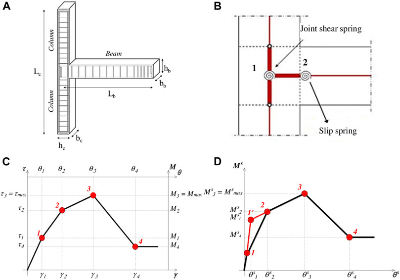
FIGURE 1. Scheme of the 2D joint under consideration (A); sketch of the used “scissors model” (B); multilinear shear stress-strain (or moment-rotation) law assigned to spring 1(C); multilinear moment-rotation law assigned to spring 2(D).
In the macro-modelling approach, frame elements and fiber discretization of the cross section were used for beams and columns, and the “scissors model” (Alath and Kunnath, 1995) was adopted for the joint element, which is generally preferred to other models due to its ease of implementation in several computer codes.
Figure 1B shows a scheme of the “scissors model”, in which the two main mechanisms governing the overall behavior of the RC joints are considered by means of two nonlinear rotational springs in series; in particular, spring 1 accounts for the shear deformation of the panel, while spring 2 represents the “fixed-end-rotation” of the beam due to the debonding of the longitudinal steel rebars at the beam-joint interface. Spring 1 connects a master node and a duplicated slave node located at the same position in the middle of the panel zone; these nodes are connected to the beam and the column members through rigid links.
The numerical analyses presented in Grande et al. (2021) as well as those described in this paper were carried out by using the open-source finite element platform “OpenSees” (McKenna et al., 2010).
The two rotational springs introduced to simulate the behavior of the joint panel were modelled through the “Pinching4 Uniaxial Material”, which is based on a multilinear moment-rotation (M-θ) backbone law. The M-θ laws introduced for the two rotational springs are directly derived from multilinear shear stress-strain (
It is worth highlighting that, in the present study, the authors focus on the proper identification of the parameters characterizing the multilinear τ-γ constitutive law assigned to the joint shear rotational spring 1 (to be converted into an M-θ relationship). Indeed, the experimental tests considered in the analyses discussed in the following sections are mostly related to beam-column assemblages experiencing the joint shear failure and, hence, their numerical modelling is generally affected by the activation of the spring 1. However, more details about the modelling of the rotational spring 2, omitted herein for the sake of brevity, can be found in Grande et al. (2021).
As shown in Figure 1C, the multilinear law is completely defined by four points identifying the main phases of the joint shear behavior, i.e.: the cracking of the joint attained at the shear stress τ1, the pre-peak phase (acting until the pre-peak stress τ2), the attainment of the peak strength τ3, the softening branch with the residual strength value, τ4, and a final constant trend. In literature, this relationship has been repeatedly adopted in several studies (De Risi et al., 2016), (Jeon et al., 2015), (Celik and Ellingwood, 2008), but different choices were made in the estimate of the key
In Shin and LaFave (2004), the proposal by Uzumeri (1977) was selected to estimate the shear stress value τ1, which is expressed by:
Where:
- fc (MPa) is the cylinder compressive strength of concrete;
- σj (MPa) is the ratio between the column axial load (N) and the corresponding cross-section area (bc hc) of the column (Figure 1A).
Table 1 provides the equations describing the five models taken into account to estimate the maximum shear stress (τ3 = τmax), directly written for the investigated 2D joints without transverse steel reinforcement. Among them, models 2 to 4 were developed by using a mechanical approach based on a strut-and-tie mechanism, whereas model 1 and model 5, very similar to each other, were empirically derived. More details, omitted here for the sake of brevity, can be found in Grande et al. (2021).
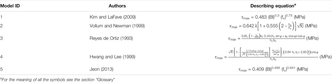
TABLE 1. Selected literature models for the estimate of peak shear stress τ3 = τmax.
For what concerns the remaining shear stresses τ2 and τ4, and the four shear strains (γ1, γ2, γ3, γ4), Table 2 lists the models selected from the literature which provided specific indications.
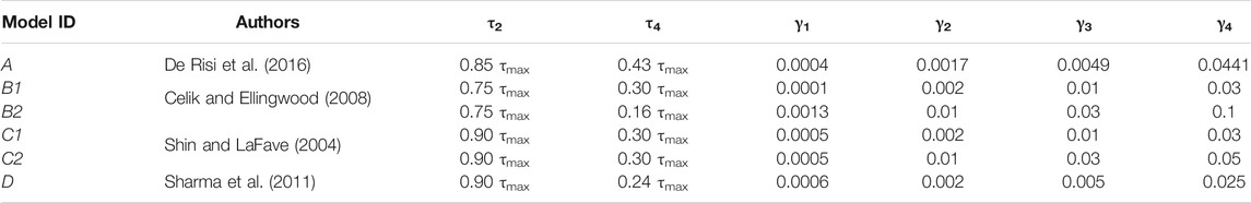
TABLE 2. Selected literature models providing values of τ2, τ4, γ1, γ2, γ3, γ4.
As observed, the values of τ2 and τ4 are given as a percentage of the maximum shear strength τ3, while the suggested values for the shear strains γ1, γ2, γ3, γ4, were calibrated on experimental basis. Unlike model A and model D, Celik and Ellingwood (2008) and Shin and LaFave (2004) provided a range of values for the shear strains γi. Therefore, the minimum (models B1 and C1) and the maximum (models B2 and C2) values of the range were reported in Table 2.
As mentioned earlier, the implementation of the τ-γ constitutive laws into the OpenSees numerical framework requires the conversion of the shear stresses into the moments Mj and the shear strains into the rotations θj of the joint shear spring. The rotation of the spring θj can be assumed equal to the joint panel strain γj, whereas the bending moment Mj is obtained from the joint shear stress τj according to Eq. 2:
which is obtained by using a simple equilibrium equation of the forces acting on the joint panel (Grande et al., 2021).
In Eq. 2, τj (MPa) is the shear stress of the multilinear law; A (mm2) is the joint cross-section area; jdb (mm) is the beam internal lever arm; hc (mm) is the height column cross-section: Lb (mm) is the beam length; Lc (mm) is the column length.
Numerical Analyses: Outcomes of the Previous Research and Insights
In Grande et al. (2021) preliminary numerical analyses were performed by considering an experimental database assembled from the literature, including a set of fifteen cyclic tests performed on specimens representative of typical exterior beam – column joints. In order to avoid eventual uncertainties and heterogeneity related to the simulated tests, the collected specimens were rather similar in terms of geometric configurations, test set-ups, load conditions, loading procedures and observed failure modes. This is the case of: 1) joints J01 and J05 tested by Realfonzo et al. (2014); 2) joints TU3 and TU1 by Pantelides et al. (2002); 3) joints #4, T#1, TC3, T01, T0, BS-L tested, respectively, by Clyde et al. (2000), De Risi et al. (2016), Del Vecchio et al. (2014), Hadi and Tran (2016), El-Amoury and Ghobarah (2002), Wong (2005) and Hassan et al. (2018); 4) joints C1 and C2 tested by Antonopoulos and Triantafillou (2003); e) joints J2 and O1 tested, respectively, by Shafaei et al. (2014) and Tsonos (2002).
All the analyzed joints presented a 2D-configuration, i.e., they were not provided with orthogonal beams (Figure 1A). Beams and columns were reinforced with ribbed steel bars, which were symmetrical arranged, except for the case of the specimens T_C3 (Del Vecchio et al., 2014) and J2 (Shafaei et al., 2014). No transverse reinforcement was located in the joint panel zone, in accordance with past code prescriptions. All the specimens failed by joint shear failure except for the joints TU1 (Pantelides et al., 2002) and T0 (El-Amoury and Ghobarah, 2002) experiencing in the pull (negative) loading direction the bond failure due to the slippage of the longitudinal reinforcements in the beam. More details about the assembled experimental database are reported in Grande et al. (2021).
The numerical analyses were performed by employing the multilinear law in Figure 1C for the shear behavior and that in Figure 1D for the bond-slip behavior. For the spring 1, different values of τ and γ were selected by opportunely combining each model providing the estimate of the shear strength τmax (models 1, 2, 3, 4, 5) with each model providing the other values of shear stress and strains (models A, B1, B2, C1, C2, D). Thus, the resulting 30 obtained τ-γ laws were implemented one at a time to carry out nonlinear static analyses by monotonically applying either downwards (positive direction) or upwards (negative direction) displacements at the end of the beam. The obtained results, expressed in terms of applied force vs. drift (the latter corresponding to the ratio between the displacement at the end of the beam and the beam length) were compared with the corresponding curves obtained from the envelope of the experimental hysteretic cycles up to 75% of the peak experimental force in the post-peak phase both in the positive and negative direction; this assumption was made to represent the same conventional failure for all the considered specimens.
Then, in order to estimate the scatter between the numerical and the experimental curves, the mean absolute percentage error (MAPE) between the experimental and the numerical force for each specimen was calculated by means of the following formula:
where: Fexp,i and Fnum,i are, respectively, the ith experimental force and the corresponding numerical one; n is the total number of measures considered in the analysis performed on each test specimen.
The bar chart in Figure 2 shows the six model combinations between the analytical proposals providing the shear strength τmax (models 1, 2, 3, 4, 5) and those suggesting the other values of shear stress and the strains (models A, B1, B2, C1, C2, D) for which the calculated errors on the whole monotonic curve for all the fifteen experimental joints were below the 25% threshold. The errors bars show the positive and negative deviation of the errors from the mean value computed for each model, while the corresponding coefficients of variation (CV) are reported in round brackets.
FIGURE 2. Ranking of the best models yielding a mean absolute percentage error (MAPE) calculated on all the monotonic envelopes lower than 25%.
In particular, the plot shows that three over the best six combinations include model 5 (i.e. the model by Jeon (2013) for evaluating the shear strength); similarly, two combinations entail model 1 (i.e., that proposed by Kim and LaFave (2009)) which also yields the lowest coefficients of variation. As mentioned earlier, these two models were developed by considering the same parameters (i.e., BI and fc) and the same formula at the basis of the calibration procedure (see Table 1).
At the same way, model A and model C1, respectively proposed by De Risi et al. (2016) and Shin and LaFave (2004), appear in five of the six best combinations.
Some Considerations on the Joint Shear Strength
The monotonic simulations in Grande et al. (2021) highlighted the strong correlation between the numerical evaluation of the global shear strength of joints and the correct estimate of the shear stress
where Tb is the tensile force acting in the longitudinal bars of the beam, Vcol is the column shear force, A is the cross-section area of the joint.
The scatter between the numerical and the experimental strength was calculated through the mean absolute percentage error (MAPE) as follows:
where
The bar charts in Figures 3A,B depict the errors for both the positive (“+”) and negative (“−”) direction of loading in terms of
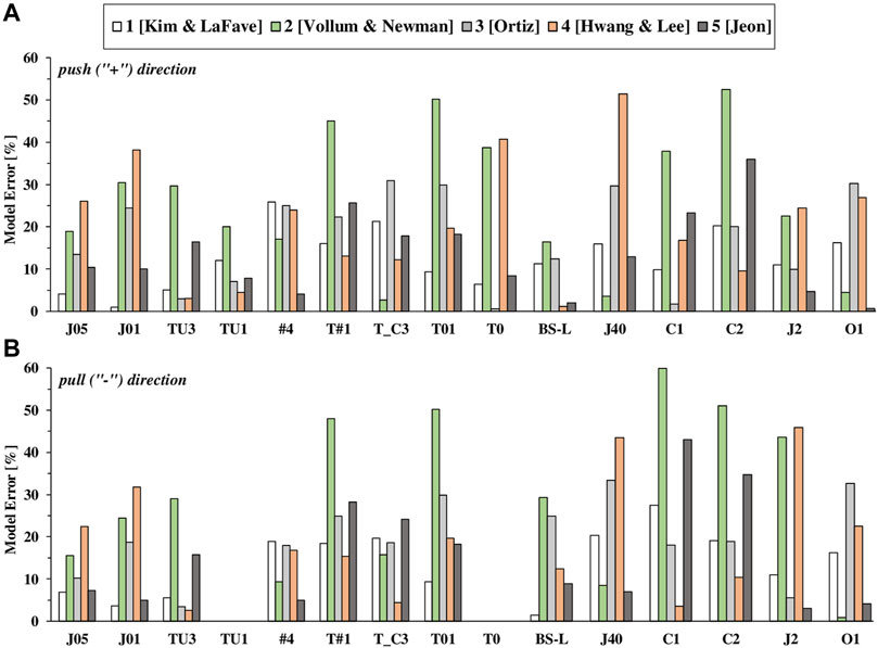
FIGURE 3. Model errors in terms of τmax for each considered experimental test: push direction (A); pull direction (B).
The bar chart in Figure 4, instead, shows the model errors in the estimate of
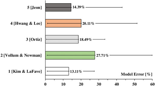
FIGURE 4. Model errors in terms of τmax calculated per each considered literature model by considering all experimental tests.
From these graphs it can be noted that the accuracy of the all models is rather variable with the considered test. Overall, model 1 (Kim and LaFave, 2009) and model 5 (Jeon, 2013) seem to provide values of the shear strength closer to the those emerged from experimental tests, since the mean errors amount to 13.11 and 14.39%, respectively (see Figure 4).
It is mentioned that these two empirical models derived from the study on the shear strength performed on a wide experimental database, considering several geometric configurations. On the contrary, the models 2, 3 and 4 were developed using a mechanical approach based on a strut-and-tie mechanism, but considering only few experimental cases investigated by the authors.
Calibration of a Constitutive model for 2D-joints
The numerical study presented in Grande et al. (2021) and briefly summarized in Numerical Analyses: Outcomes of the Previous Research and Insights was basically devoted to 1) identify the literature models best estimating the joint shear strength and, 2) find, based on the literature proposals, the multilinear joint shear stress-strain constitutive law that, implemented in the proposed model for 2D-joints, be able to provide the best simulation of then monotonic envelopes of load-displacement experimental curves.
The study presented in this paper, instead, is aimed at deriving a new constitutive model for the analysis of both the monotonic and cyclic behavior of 2D-joints, with the purpose to further improve the simulation of the considered experimental tests. To this end, a calibration procedure is carried out by considering just the mentioned experimental database concerning RC beam-column joints in 2D configuration. In particular, while the first application of the procedure specifically regards the shear strength of the joint, presented in the following, the subsequent applications are devoted to derive: 1) a multi-linear shear stress-slip law for the monotonic response, described in The Proposed Backbone Joint Shear Stress-strain Law, and 2) a model able to predict the response of 2D joints under cyclic loads, presented in Modeling of Cyclic Response of Joints – “Pinching4” Model.
Joint Shear Strength Model Prediction
The assessment of the literature models in predicting the shear strength of the experimental database, presented in the previous section, showed that the models proposed by Kim and LaFave (2009) and by Jeon (2013) provided the lowest values of MAPE (13.11 and 14.39% respectively). As observed from Table 1, both models identified the beam reinforcement index, BI, and the concrete compressive strength, fc, as the key parameters affecting the joint shear strength; the only difference between the two equations relies into the numerical coefficients calibrated by the authors based on their own accounted set of experimental cases.
In the present study, considering an experimental database containing 2D-joint configurations only, a multivariate linear regression analysis is performed by taking into account the same predictor variables (BI and fc) and the same structure of the formula used by model 1 and model 5 for deriving the shear strength:
where a, b and c are the numerical coefficients to be opportunely calibrated.
It is worth highlighting that the use of a multivariate linear regression analysis instead of a simple linear regression method allows to study the relationship between a dependent variable and more than one independent variable.
The general functional equation is expressed by an additive model expressed in a logarithmic scale as follows:
where:
- Y is the response (dependent) variable;
- Xj(j = 1,2…n) are the predictor (independent) variables;
- βj (j = 1,2…n) are the coefficients of the regression analysis.
In the literature, this functional form was employed in several empirical models for estimating the main variables affecting the shear strength of beam and column elements in RC framed structures (Jeon, 2013), (Haselton et al., 2016).
Once the numerical coefficients of the relationship are evaluated, Eq. 10 can be equivalently rewritten in the original multiplicative form:
The coefficient of determination R2 and the residual standard error σ quantify the effectiveness of the predictive model and are evaluated based on the regression analysis carried out using the form in Eq. 7.
By focusing on the prediction of the shear strength of exterior joints, the dependent variable is, of course, represented by the shear strength
whereas Eq. 8 can be converted into an expression coinciding with Eq. 6.
In order to examine the accuracy of the two predictor variables BI and fc on the response variable
Usually, a stepwise elimination process is performed until all the remaining variables are all significant at the 95% level based on the “F test”.
The regression analysis, in conjunction with the ANOVA test, was performed by considering both the positive and the negative values of the shear strength
Table 3summarizes the results obtained from the regression analysis in terms of “F test” value, root mean square error (RMSE), correlation of determination (R2) and p-value, while Table 4 shows the results of each predictor variable in terms of numerical coefficients, “t test” value and p-value.
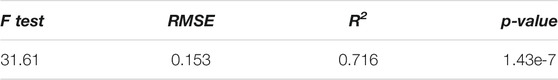
TABLE 3. Regression results for the proposed empirical model.
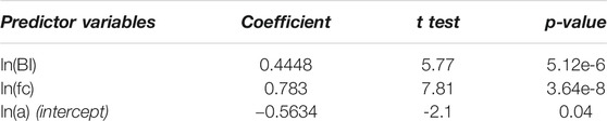
TABLE 4. Regression results for each predictor variable.
As observed, both the variables BI and fc are significant at the 95% level based on the “F test” and each of them, including the intercept (ln(a) in Eq. 9), are significant at the 95% based on the individual “t test”. Thus, the null hypothesis can be rejected for both the statistic tests; moreover, the coefficients resulting from the multiple linear regression can be deemed relevant for the purposes of the predictive capacity model.
Before definitively accepting the results derived from the multiple regression analysis, it is necessary to perform an outlier detection plan in order to identify whether the obtained model is appropriate. To this aim, the residuals are plotted against the predicted values and against the predictor variables to determine whether some data points must be eliminated to get a final model. If the residuals are distributed within a horizontal band centred around the zero, the model can be deemed accurate and it does not show any trend in overestimating or underestimating the output of the independent variable. Furthermore, the normal probability plot must be displayed to assess the normality of the distribution of the residuals. This condition is achieved if the points in the plot lie approximately on a straight line.
Figure 5A shows the residual plot against both the fitted values ln(
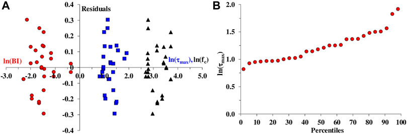
FIGURE 5. Residual plots for ln(τmax) (blue points), ln(fc) (black points) and ln(BI) (red points)(A); normal probability plot of the predicted values (B).
Therefore, the functional form of the predictive model can be expressed by Eq. 10, with the numerical coefficients derived from the ANOVA test:
that, converted into the original multiplicative form expressed by Eq. 6, provides the following predictive model for the joint shear strength:
Comparison Between the New Proposal and the Literature Models 1 and 5
By comparing the new proposal with the counterpart models by Kim and LaFave (2009)(model 1) and by Jeon (2013) (model 5), it is noted that the main difference lies in the coefficient multiplying the parameter BI and fc (= 0.569), which is higher than those of the two literature models (0.483 and 0.409, respectively); the coefficient term (0.445), representing the power of BI, is higher than that provided by Kim and LaFave (0.3), but lower than that provided by Jeon (0.495); the coefficient representing the power of fc (0.783), instead, is slightly higher than that found by Kim and LaFave (0.75), but lower than that proposed by Jeon (0.941). Of course, differences in the found numerical coefficients are strictly related to the experimental database used for the calibration procedure; to this purpose, as already mentioned, the new proposal was specifically found by considering an experimental database including a homogeneous set of RC exterior joints.
In order to compare the accuracy of the proposed strength model with that of the counterpart formula, the bar chart in Figure 6 shows the mean errors in terms of
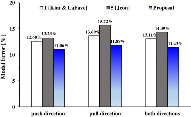
FIGURE 6. Comparisons between the new proposal and Models 1 & 5 in terms of mean errors calculated according to MAPE on all the considered experimental tests.
As observed, all the three models always provide the highest errors in the pull loading direction; however, the application of proposed model yields an overall error reduction of about 13–15% and 20–30% with respect to model 1 (Kim and LaFave, 2009) and model 5 (Jeon, 2013), respectively.
Finally, in Figure 7 the theoretical values
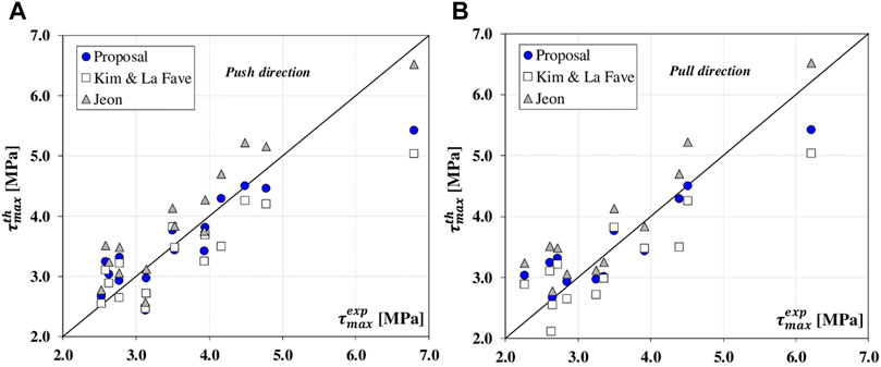
FIGURE 7. Numerical vs experimental τmax values: comparisons between the new proposal and Models 1 & 5: push loading direction (A); pull loading direction (B).
As shown, the application of the new strength model leads, except for a few cases, to the best agreement between prediction and tests, with points (blue circles) mostly distributing about the bisector line. Conversely, points related to the application of the model by Kim and LaFave (2009) (white squares) are mostly distributed below the bisector line, thus indicating conservative predictions; an opposite trend, instead, is observed for points referred to the use of the formulation by Jeon (2013), generally providing non-conservative predictions.
The Proposed Backbone Joint Shear Stress-strain Law
By following the development of a sound analytical model for the estimate of the maximum shear stress (τmax = τ3), a new backbone τ – γ law was identified by properly defining the remaining stress and strain parameters of the multilinear relationship assigned to the rotational spring 1 (Figure 1C).
In particular, the stress values (τ1, τ2, τ4) were determined by both following the indications provided from literature studies and accounting for the conclusions drawn from the preliminary numerical analyses published in Grande et al. (2021). The strain parameters (γ1, γ2, γ3, γ4), instead, were identified by carrying out new monotonic numerical analyses in which their associated values were varied within specific ranges chosen by authors. Then, by computing the errors emerged from the numerical vs experimental comparisons in terms of force – drift monotonic envelopes, the best set of γi parameters was identified.
It is worth highlighting that the whole calibration procedure, better detailed in the following sections, consists of, firstly, defining the values of the stress parameters, and, secondly, identifying the best values for the strains γi among the investigated ones. Of course, the two steps of the applied procedures are not decoupled, since the percentage errors emerged from the sensitivity analyses are affected on both the stress and strain assessments.
Definition of the Stress Parameters (τ1, τ2, τ4)
Cracking Shear Strength τ1
Based on the examined literature studies, the cracking shear strength τ1 can be reasonably estimated through the formula proposed by Uzumeri (1977) (see Eq. 1). In particular, the results of the preliminary numerical analyses published in Grande et al. (2021), which were performed by implementing the 30 τ-γ model combinations briefly described in Numerical Analyses: Outcomes of the Previous Research and Insights, highlighted that this first stress point can be roughly set, on average, to 57% of τmax.
Pre-Peak Strength τ2
The pre-peak strength τ2 can be assumed equal to 0.85τmax, according to the model proposed by De Risi et al. (2016), which showed the best agreement in predicting the pre-peak branch of the monotonic experimental envelopes (Grande et al., 2021). Moreover, since the minimum pre-peak strength assessed from the literature models is 0.75τmax (as proposed by Celik and Ellingwood (2008)), while the maximum value is 0.9τmax (model by Shin and LaFave (2004) and model by Sharma et al. (2011)), an average value between the two ends of the range (i.e., τ3 = 0.85τmax) can reasonably assumed.
Residual Strength τ4
The residual strength point τ4 of the backbone law is assumed equal to 0.3τmax which is the value approximately suggested by the most of considered literature models (Shin and LaFave, 2004; Sharma et al., 2011; Celik and Ellingwood, 2008) (see also Table 2) and fitting quite well the experimental monotonic curves in the post-peak phase (Grande et al., 2021).
The second column of Table 5 summarizes the four τi stress values identified by authors for the proposed constitutive law.
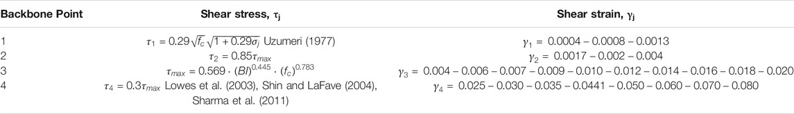
TABLE 5. Selected shear stress values and proposed ranges for γi parameters.
Definition of the Strain Parameters (γ1, γ2, γ3, γ4)
A higher uncertainty affects the strain parameters of the τ – γ relationship, since the proposed values from the literature are merely derived from experimental observations on each individual test, and do not depend on neither particular geometric or mechanical properties nor other theoretical considerations. However, the assessment of the monotonic analyses in terms of load-drift published in Grande et al. (2021) provided preliminary indications on the range of strain values which best meet the experimental results. Thus, a sensitivity analysis was carried out on all the 15 experimental tests, with the aim to identify a set of strain parameters to propose in the τ – γ constitutive model for exterior joints.
Table 5 provides the four proposed ranges of strains to assess (γ1, γ2, γ3, γ4) which were associated to the corresponding backbone points. The motivations for investigating such ranges are provided in the following.
Strain γ1
Regarding the strain corresponding to the cracking shear strength τ1, investigating only three values was considered sufficient for the purpose of the study; indeed, the monotonic analyses previously performed by implementing the 30 mentioned model combinations showed that a larger variation of this parameter does not lead to a significant scatter in terms of errors calculated between experimental and numerical enveloped in the first loading branch. In detail, these analyses highlighted that, relatively to γ1 parameter, the lowest errors were generally obtained by considering model B2 in which the value γ1 = 0.0013 (upper end of the range provided in Table 5) coincides with the upper end of the range proposed by Celik and Ellingwood (2008); such a value is also the highest among those proposed by the various authors (see Table 2). However, numerical analyses related to some few tests showed that the first branch of the experimental monotonic envelope was better reproduced by setting γ1 to 0.0004 (lower end of the range provided in Table 5); such a value is that proposed by De Risi et al. (2016) but it is not significantly different from other proposals (Shin and LaFave, 2004), (Sharma et al., 2011) (see Table 2). Finally, γ1 = 0.0008 in Table 5 is the average value of the range and represents a third alternative considered by authors.
Strain γ2
Regarding the strain corresponding to the pre-peak strength τ2, it is worth mentioning that the previous analyses highlighted that the implementation of the models B2 and C2 in Table 2, both suggesting γ2 = 0.01, led to the highest scatter in terms of errors between the numerical drift and the experimental one; conversely, the adoption of lower γ2 values, such as those provided by the other models, showed to provide better simulations. Therefore, the first two γ2 values included in the range reported in Table 5 coincide, respectively, with those of model A (De Risi et al., 2016) and models B1 (Celik and Ellingwood, 2008), C1 (Shin and LaFave, 2004) and D (Sharma et al., 2011). The upper end of the range, instead, was arbitrarily chosen by the authors with the aim to consider a third alternative; as shown later, this value was found to be optimal in carrying out the numerical analyses.
Strain γ3
With respect to γ1 and γ2, the strain corresponding to the peak stress, γ3, is characterized by greater uncertainty; indeed, the previous numerical analyses performed on the considered experimental tests have highlighted the wide range of values that such parameter can assume to fit the experimental data well. The same literature models in Table 2 propose very different values for γ3. However, it is worth mentioning that the previous analyses showed that, as for γ2, the implementation of the models B2 and C2 in Table 2, both suggesting γ3 = 0.03, led to the highest scatter in terms of errors between the numerical drift and the experimental one. Conversely, the models yielding the lowest errors were found to be models B1 and C1 (both suggesting γ3 = 0.01), in the push loading direction, and models A and D (suggesting γ3 = 0.0049 and γ3 = 0.005, respectively) in the pull loading direction. Therefore, in order to cover the widest range of possible values, γ3 spans from 0.004 (value close to the minimum one proposed in literature, equal to 0.0049 (De Risi et al., 2016)), to 0.02 (the highest value found from the previous numerical analyses fitting some experimental curves well). Within this range, a thickening of the values was considered towards the lower end, where the higher uncertainty was identified in the numerical analyses; conversely, by moving towards the upper end of the range, a lower number of values were considered, being less likely.
Strain γ4
As for γ3, high uncertainties affect the correct identification of the strain γ4 corresponding to the residual strength τ4. These are related, on one hand, to the test procedures used in some experimental investigations (as that carried out by Realfonzo et al. (2014), where tests were stopped at a predetermined conventional collapse in order to not significantly damage the specimens) and, on the other end, to the significant scatter of values proposed in the literature models (see Table 2). Therefore, in this case, the lower end of the range coincides with the minimum value suggested in literature (γ3 = 0.025 (Sharma et al., 2011)); then, such a value was increased up to 0.050 (value adopted by model C2 (Shin and LaFave, 2004)) by also including the other literature proposals. Finally, in order to account for experimental cases in which high values of drift were experienced, the remaining values of γ4, equal to 0.06, 0.07 and 0.08, were also taken into consideration.
Sensitivity Analysis and Results
In order to assess the influence of each γi parameter on the global response in terms of force – drift results, the sensitivity analysis was performed by varying every single value of the strain parameter within the predetermined range, thus requiring a hard computation effort. Indeed, a total of 21600 monotonic analyses were carried out by considering the 720 values of the strain parameters [= (#3
Each of the monotonic curves resulting from the sensitivity analysis was compared to the experimental envelope of each test and the MAPE value was calculated according to Eq. 3.
It is highlighted that the errors between the ith experimental force and the corresponding numerical one were calculated considering the total length of the numerical monotonic curve (i.e., until the point τ4 – γ4, or, equivalently, until the final point of the experimental curve).
For each experimental test, the combination of (γ1, γ2, γ3, γ4) minimizing the mean absolute percentage error on the monotonic envelope was, then, identified.
The resulting combinations are shown in Table 6 for each experimental test, together with the related percentage error. The last row of Table 6 also reports in bold italics the combination of “mean” γi, i.e., the set of γi obtained by averaging the values obtained from all the 15 experimental tests, together with the corresponding mean value of the errors. Such set of γi values is that proposed by the authors in conjunction with the stress parameters τi to define a new backbone joint shear stress-strain law to implement and validate in the numerical analyses described in the following section. For better clarity, the four couples of (τi – γi) parameters of the proposed law are summarized in Table 7.
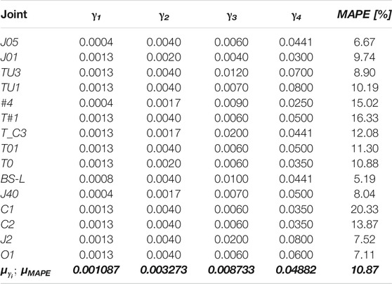
TABLE 6. Strain parameters minimizing the mean absolute percentage errors.

TABLE 7. Shear stress and strain parameters of the proposed constitutive law.
Validation of the Proposed τ – γ Law
In order to check the accuracy of the proposed model, new monotonic analyses were carried out by implementing the proposed τ – γ law in the OpenSees computer code, both in the positive and negative direction of the loading. Then, the MAPE value between the experimental and numerical curve was calculated by applying Eq. 6 over the whole monotonic envelope of each test.
In Table 8, the errors per each test related to the implementation of the proposed constitutive law (namely “proposed model”) are compared with those obtained by considering the best three literature τ – γ models identified in Numerical Analyses: Outcomes of the Previous Research and Insights, i.e., “model 5A”, “model 1A” and “model 5C1” (see the ranking in Figure 2). Furthermore, the errors resulting from considering the optimal set of γi parameters − found test by test in the minimization error procedure (see Table 6) − in place of the proposed average values in Table 7, are reported for a better comparison (see column “optimal solution” in Table 8).
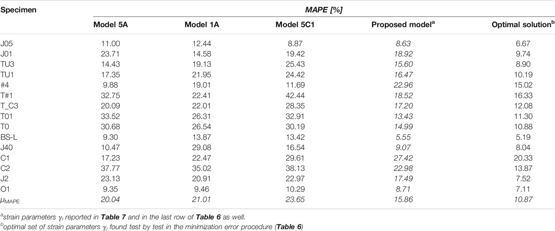
TABLE 8. Mean absolute percentage errors and their mean values calculated for: a) the best three literature models (5A, 1A and 5C1); b) the proposed model, and c) the optimal solution.
As expected, test by test the MAPE values related to the “proposed model” are higher than those derived by the “optimal solution”; on average, the mean error computed on all the experimental tests (μMAPE) is about 45% greater (compare 15.86% with 10.87% in the last raw of Table 8). In particular, it is observed that for some specimens (specifically, J05, T#1, T01, BS-L, J40, O1), there is not a large scatter between the “proposed model” and the “optimal solution”, while some others (J01, TU3, #4, C1, C2, J2) show a higher difference in the error between these two models.
The mean error provided by the “proposed model” is, however, lower than that derived from the literature models 5A, 1A and 5C1, which show μMAPE values equal to 20.04, 21.01 and 23.65%, respectively.
Of course, in some tests the error for the “proposed model” is higher than that related to the literature models. This is the case of: a) the model 5A which provides better results for the tests TU3 (Pantelides et al., 2002), #4 (Clyde et al., 2000), C1; b) the model 1A which shows lower errors for the tests J01 (Realfonzo et al., 2014), #4 (Clyde et al., 2000), C1 (Antonopoulos and Triantafillou, 2003), and c) the model 5C1 furnishes better results for the specimen #4 (Clyde et al., 2000). Only in the case of the joint #4 (Clyde et al., 2000), the “proposed model” works worse than all the three literature models. However, it is worth mentioning that the percentage errors related to the literature models, published in Grande et al. (2021) and provided in Table 8 for the sake of comparison, have been computed until the 75% of the maximum strength, while the errors of both the “proposed model” and the “optimal solution” are evaluated considering the whole monotonic envelope.
Finally, Figure 8 shows the resulting force – drift monotonic curves plotted for all the 15 specimens. In particular, in each graph the red curve and green one represent the monotonic envelope numerically obtained by implementing the τ – γ law identified as “optimal solution” and “proposed model”, respectively; the black dotted curve, instead, is the experimental monotonic envelope.
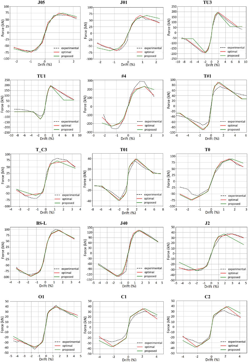
FIGURE 8. Numerical vs Experimental comparison of the monotonic envelopes considering the “optimal solution” (red curve) and the “proposed model” (green curve).
The Figure clearly highlights the greater accuracy in matching the experimental behavior when the “optimal solution” is implemented in the numerical simulations, but the “proposed model” also provides good results for all the analyzed joints.
Both the numerical curves match the first elastic branch of the experimental envelope better than the softening phase; this issue is also common to all the numerical models investigated in the previous study (Grande et al., 2021). In fact, the main difference between the “optimal solution” and the “proposed model” stands after the peak point for most of the cases. As also shown from the errors in Table 8, the proposed numerical model (green curve in Figure 8) meets well the experimental outcomes in the following cases: J05, BS-L, J40, O1. On the other hand, the worst results are shown for the tests #4, T#1, TC_3, C1 and C2. Even in this analysis, the negative envelopes of the specimens TU1 and T0 are related to the nonlinear rotational spring describing the anchorage failure of the bottom bars at the beam-joint interface.
It is noticed that, in the case of the joints showing the higher errors, the main difference between the numerical and the experimental results relies in the values of the peak force, i.e. in the maximum shear strength. This aspect confirms that the assessment of this parameter is a crucial preliminary step in the definition of the shear behavior of beam – column joints.
Moreover, in the cases of joints TU3, TU1, T#1, T01, the “proposed model” is characterized by a constant trend after the residual strength point (τ4-γ4 in the constitutive law) since the corresponding experimental envelopes experienced high excursions in terms of drift in the post-peak phase.
Modeling of Cyclic Response of Joints : “Pinching4” Model
The modelling of the cyclic behavior represents a key aspect in the study of the seismic performance of the RC beam-column joints and is characterized by a greater complexity with respect to the simulation of the monotonic response. To this aim, the “pinching4” uniaxial material model (see Figure 9), available in the OpenSees library (McKenna et al., 2010), and developed by Lowes et al. (2003), was still used to set the parameters governing the hysteresis rule and pinching effect. This model has been widely used in several studies available in literature to simulate the hysteretic behavior of shear critical elements like beam – column joints or infilled frames (De Risi, 2015).
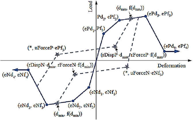
FIGURE 9. “Pinching4” material model (adapted from Lowes et al. (Kim and LaFave, 2012)).
The model is based on a multilinear envelope response (backbone curve) and a trilinear unload – reload path, as illustrated in Figure 9. The cyclic degradation is simulated by three damage rules, that is, unloading stiffness degradation, reloading stiffness degradation (i.e. deterioration in strength developed in the vicinity of the maximum and minimum deformation demands) and strength degradation (i.e. deterioration in strength achieved at previously unachieved deformation demands).
Figure 10 shows the different effect of these three damage modes on the hysteretic response of the material.
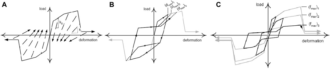
FIGURE 10. Damage modes of the “pinching4” material: unloading stiffness degradation (A); reloading stiffness degradation (B); strength degradation (C) (Genesio, 2012).
Each of the three hysteretic damage modes is characterized by a modified version of the damage index proposed by Park and Ang (1985), dependent on the displacement history and the accumulated energy, as follows:
where:
- the subscript i refers to the current displacement increment;
- δi is the damage index (0 in case of no damage, 1 in case of maximum damage);
- αj are parameters required to fit the damage rule to experimental data;
- Ei is the accumulated hysteretic energy;
- Emonotonic is the energy required to achieve under monotonic loading the deformation that defines failure;
- defmax and defmin are the positive and negative deformations that define failure;
- dmax and dmin are the maximum and minimum historic deformation demands;
- δlim is the maximum possible value of the damage index;
- gE is a multiplication factor used to define the maximum energy dissipation under cyclic loading.
The same basic equations are used to describe deterioration in strength, unloading stiffness and reloading stiffness. For the case of stiffness degradation (Figure 10A):
where: ki is the current unloading stiffness; k0 is the initial unloading stiffness for the case of no damage; δki is the current value of the stiffness damage index.
The same relationship describes the envelope strength degradation (Figure 10C), as follows:
where: fmax,i is the current envelope maximum strength; fmax,0 is the initial envelope maximum strength for the case of no damage; δfi is the current value of the strength damage index.
The case of reloading stiffness degradation (Figure 10B) is defined by applying an increase in the maximum (decrease in the minimum) historic deformation demand:
where: dmax,i is the current deformation that defines the end of the reload cycle for increasing deformation demand; dmax,0 is the maximum or minimum historic deformation demand; δdi is the current value of the reloading – strength damage index.
The damage rule of Eq. 12 requires the definition of 4 parameters (αj) which must be calibrated for each of the three damage indices on the basis of experimental data. In the “pinching4” model, these αj parameters are replaced by proper degradation model parameters to be defined for each damage index (δki, δfi, δdi); all these 15 parameters are indicated in Table 9.
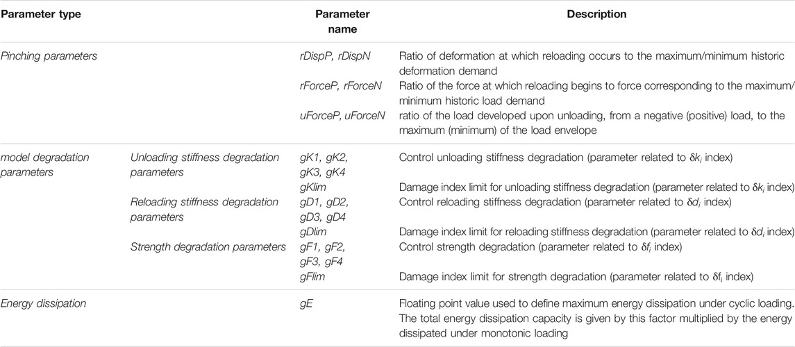
TABLE 9. Pinching4” material model parameters and their role.
Also, as observed in Table 9, the “pinching4” model requires the definition of other parameters, i.e.: 1) gE, already introduced in Eq. 15, and 2) three couples of parameters (rDispP, rDispN; rForceP, rForceN; uForceP, uForceN) describing the pinching behavior of the unload-reload path in Figure 9.
It is worth mentioning that the correct setting of these 22 parameters characterizing the material model (specifically, 15 degradation parameters + “gE” + 6 unloading–reloading pinching parameters), is a key task in the numerical simulation of the joint cyclic response. To this purpose, several studies were published in the literature, in which the calibration of these parameters was always based on a fitting process of experimental cyclic responses of beam-column joints. In this paper, the studies performed by Lowes and Altoontash (2003), Theiss (2005), Hassan (2011), De Risi (2015), Jeon (2013) were taken under consideration for the definition of the “pinching4” material model. The main details of these studies are provided in the following section.
Selected Literature Studies
In each selected literature study the researchers defined a set of “pinching4” parameters even though generally calibrated by using their own experimental data. In particular, the study by Lowes and Altoontash (2003) represents one of the first attempts to provide specific indications on the hysteretic rules defined by the “pinching4” material model. The proposed unload-reload path and the damage law were assessed through the comparison between the simulated and the observed response for a series of four joint sub-assemblages with different design details. The backbone envelope was defined through the modified compression field theory (MCFT) approach proposed by Vecchio and Collins (1986). Experimental data provided by Stevens et al. (1991) were, then, used to define the response under cyclic loading. These data showed an extremely pinched shear stress-strain behavior, which was attributed to the opening and closing of cracks in the concrete-steel composite. The numerical simulations showed that the proposed model represented well the fundamental characteristics of the observed response, including energy dissipation within the joint and the shear failure mode. However, due to the limited number of experimental tests investigated by the authors, the accuracy of the model should be further assessed for a higher number of joints.
Theiss (2005) investigated five laboratory tests previously carried out by Walker (2001) and Alire (2002). Different cyclic analyses were performed, employing simulation and no simulation of the joint’s strength and stiffness deteriorations under cyclic loading. The results showed that simulating the strength and stiffness deteriorations had a significant impact on the global hysteretic response of the joints, especially in terms of maximum drift demands. The effect of the joint modeling was also evaluated through dynamic analyses on a three-story RC frame building.
The study by Hassan (2011) aimed at evaluating the seismic performance of four full-scale corner beam-column joint sub-assemblies until total collapse. The model incorporates the effect of axial load level, overturning seismic moment, joint aspect ratio, joint failure mode and the post-shear damage residual axial capacity. To validate the appropriateness of the proposed joint model, six additional unconfined exterior and corner tests were selected from literature and investigated through numerical simulations.
The study by De Risi (2015) focused on proposing a modelling approach for exterior RC joints under cyclic loading in order to assess the seismic vulnerability of existing RC buildings typical of Italian/Mediterranean building stock, and to evaluate the impact of joints’ response on such a performance. To this purpose, the calibration of the key parameters governing the joint panel hysteretic behavior was based on an experimental database including 10 tests of which 2 were performed by the same author; from the calibration procedure, the mean values of the parameters calibrated from each test were finally proposed. In particular, the applied procedure was performed starting from the experimental shear stress-strain backbones and minimizing the error in terms of dissipated energy between the numerical and the experimental responses. No degradation in strength was introduced (namely all gF parameters in Table 9 were set equal to zero) since it was already included in the backbone of the joint response obtained from the experimental data.
Finally, the study by Jeon (2013) was based on the most complete experimental database, which gathered 28 exterior sub-assemblages from literature. The mean values of the “Pinching4” material parameters, extracted from the model validation in terms of strength, stiffness and energy dissipation, were then utilized in the simulations of RC structures for a probabilistic risk assessment.
Table 10 shows the values of the pinching parameters proposed by the selected literature studies. From this table, the following considerations can be made:
- in most of the cases, the pinching parameters (rDisp, rForce, uForce) are assumed to be equal − in absolute value − between the positive and negative unload – reload path; only Hassan (2011) proposed different values between the two branches (in particular, rForceP = 0.35 and rForceN = −0.40, whereas uForceP = −0.10 and uForceN = −0.40);
- the models by Lowes and Altoontash (2003), De Risi (2015) and Jeon (2013) assumed the unloading stiffness damage to be a function of the displacement history only, since the parameters gK2 and gK4, related to the energy accumulation damage, are set equal to zero. The same observation can be made for reloading stiffness degradation parameters; in this case, also the model by Theiss (2005) shows that the stiffness loss is determined primarily by the maximum deformation demand (dmax) (gD2 = 0.005; gD4 = 0);
- both the unloading and the reloading stiffness damage indices limits (gklim and gDlim) assumed similar values among all the models; in fact, the maximum value of gklim is equal to 0.99 (Theiss, 2005), (Hassan, 2011) and the minimum is 0.89 (Lowes and Altoontash, 2003), while gDlim assumes a maximum of 0.99 (Theiss, 2005), (Hassan, 2011) and a minimum of 0.95 (Lowes and Altoontash, 2003; Jeon, 2013);
- the displacement history is taken as main factor of the strength degradation index for the models by Lowes and Altoontash (2003), Theiss and Jeon (gF2 and gF4 equal to zero) (Theiss, 2005; Jeon, 2013);
- the strength degradation limit (gFlim) is equal to 0.99 for the models by Theiss (2005) and Hassan (2011) (note that this limit value is also assumed for the other damage indices by these authors), whereas much lower values are assumed by the models by Lowes and Altoontash (2003), and Jeon (2013) (0.13 and 0.25, respectively);
- as mentioned earlier, the strength degradation parameters assumed by De Risi (2015) are all set equal to zero, i.e., no strength degradation is included in this model. Indeed, due to these parameters, a reduction in the envelope curve of the hysteretic cycles would have been shown, leading to a mismatch if the monotonic backbone had been previously calibrated through specific analyses and assumptions as done by De Risi (2015); the author proposed the multilinear response envelope, based on some experimental tests, before the definition of the degradation laws concerning the cyclic behavior of joints;
- the energy dissipation factor gE is assumed equal to 10 by all the models, with the exception of the model by Theiss (2005), which proposed an energy multiplication factor equal to 2.
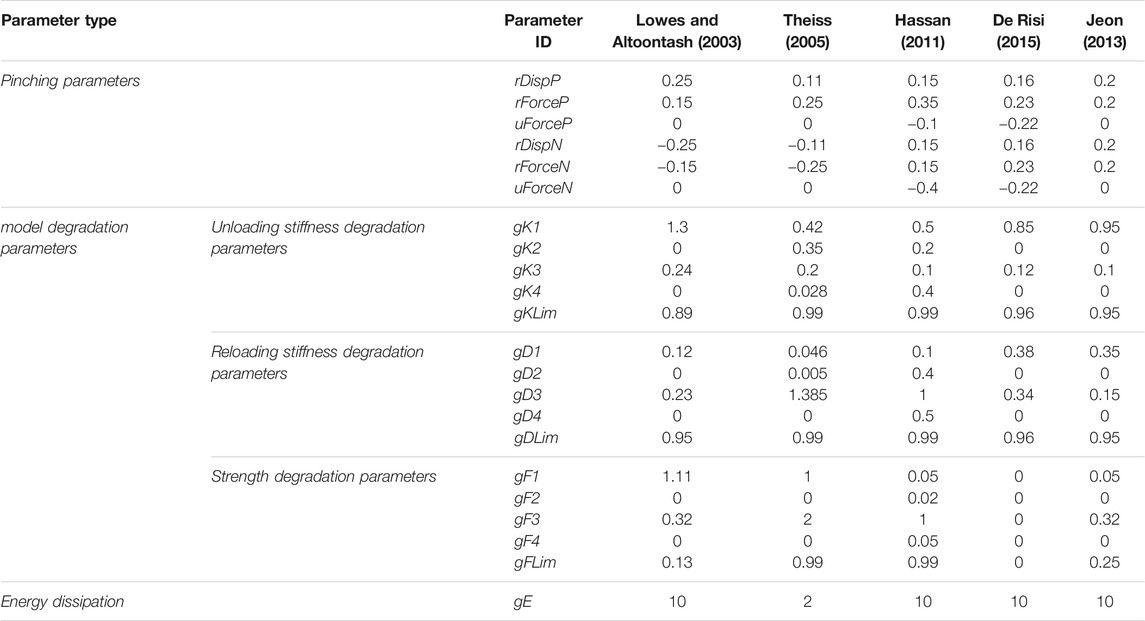
TABLE 10. Values of the “Pinching4” material parameters selected from the literature.
Assessment of the Model Parameters Proposed in Literature
The considerations made on the literature values assigned to the “pinching4” model parameters represent a useful starting point for carrying out cyclic analyses on the experimental tests available in the database. Therefore, the obtained results have allowed, on one hand, to identify the literature proposal fitting the experimental best and, on the other end, to catch valuable indications on how to properly modify the values of some “pinching4” model parameters.
To this purpose, the finite element model geometry used to simulate the monotonic envelope of the experimental joints, was again considered to carry out cyclic analyses for the same set of 15 specimens in the OpenSees platform (McKenna et al., 2010).
Even in this case, the macro – modeling approach adopted the “scissors model” to simulate the joint element, with the two rotational springs 1 and spring 2 in series, representing the shear behavior of the joint panel and the bond – slip mechanism at the beam – joint interface. In particular, the multilinear moment – rotation (M–θ) law in Figure 1C was adopted to describe the envelope backbone of the shear rotational spring, of which the key parameters were derived from the τ and γ values previously calibrated by the authors (see Table 7).
The “pinching4” uniaxial material model was, hence, assigned to the two rotational springs. Of course, besides the implementation of the backbone envelope in terms of moment-rotation multilinear laws, the “pinching4” material model requires, for cyclic analyses, the mentioned additional 22 parameters describing the unloading-reloading path, the strength and stiffness degradation and pinching effect (see Table 9).
Therefore, for each of the 15 experimental specimens, a set of 5 cyclic analyses were carried out by implementing the corresponding 5 sets of cyclic degradation parameters listed in Table 10.
It is worth highlighting that that no strength degradation was considered in all the 5 models, meaning that the strength damage index parameters (gF1, gF2, gF3, gF4, gFlim) were always set equal to zero whatever the accounted model. Indeed, like the numerical study performed by De Risi (2015), even in this work the monotonic envelope of each joint has been separately calibrated by performing specific monotonic analyses. The introduction of the strength loss phenomenon, indeed, would have reduced the envelope backbone, leading to a worsening with respect to the experimental monotonic curve.
In order to assure a perfect correspondence between numerical and experimental curves, the cyclic analyses were performed by implementing, for each single experimental test, the same displacement history described in literature by the authors.
Results and Discussion
In order to identify the model which best approximate the cyclic behavior of the tests, an assessment was carried out on the basis of the difference between the numerical and the experimental response in terms of dissipated energy (Ed,i) and stiffness degradation (Ki) at each cycle. In fact, these are the properties mainly controlling the shape of the hysteretic loops and their evaluation is a relatively simple issue in the post – processing phase of the force – drift cyclic response. In particular, by summing up the area enclosed by each force-displacement cycle, the total cumulative dissipated energy was obtained, which obviously increases with the imposed displacement. On the other hand, the secant stiffness Ki was calculated through the relationship proposed by Mayes and Clough (1975) as follows:
where: F+max,i and F−max,i are the peak lateral forces applied to the beam in the two directions of loading; D+max,i and D-max,i are the corresponding displacements.
Unlike the cumulative energy, the secant stiffness decreases with imposed displacement.
To compare the accuracy of the numerical simulations resulting from the implementation of the five sets of “pinching4” model parameters, the mean absolute percentage error was calculated between the experimental and the numerical values for both energy and stiffness at each cycle by applying the following equation:
where n is the total number of measures in terms of energy and stiffness available for each specimen,
The MAPE values emerged from the analysis are reported in Table 11 for both energy and stiffness parameters; the mean value (μMAPE) calculated per each model on all the experimental tests is also provided in the last row of Table 11.
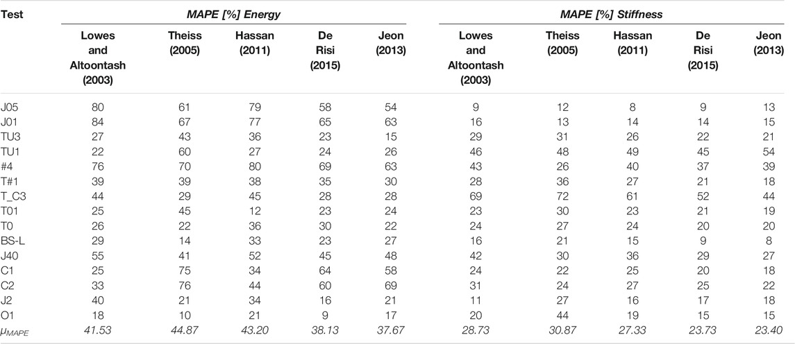
TABLE 11. Mean absolute percentage errors for energy dissipation and stiffness degradation.
As observed, the model by Jeon (2013) yields the lowest μMAPE values both in terms of energy and stiffness, being equal to 37.67 and 23.40%, respectively. In the ranking, the model by De Risi (2015) follows, providing overall mean values equal to 38.13% for the dissipated energy and 23.73% for the stiffness degradation. For both the properties, the model leading to the highest mismatch is the model by Theiss (2005).
By analyzing the tests case by case, some observations can be made regarding the joints J05 and J01 (Realfonzo et al., 2014), since they are characterized by high values of errors for the energy, but very low values for the stiffness if compared to corresponding results found for the other tests. This particular outcome is probably due to the fact that the experimental data of the entire cyclic load history were available for these tests. Thus, the analysis on the dissipated energy and stiffness degradation was made possible also for the first small imposed displacements, which have been proven to furnish the highest mismatch in terms of loop width and, consequently, in terms of energy dissipation. No substantial differences are observed in terms of secant stiffness at each cycle, since the monotonic backbone of the numerical models provided a good approximation with the experimental envelope.
Moreover, it is highlighted that, the cases that already had showed the highest errors in terms of monotonic envelopes (see §5) are also characterized by high errors in terms of energy dissipation and stiffness loss (see joints #4, T#1, T_C3, C1, C2 in Table 11). This observation remarks the importance of defining a proper monotonic backbone curve before studying the hysteretic cyclic behavior.
Figure 11 and Figure 12 depict the cumulative dissipated energy and the stiffness degradation, respectively; for each test, all the five numerical outcomes are displayed and compared among them and with the experimental trend as well.
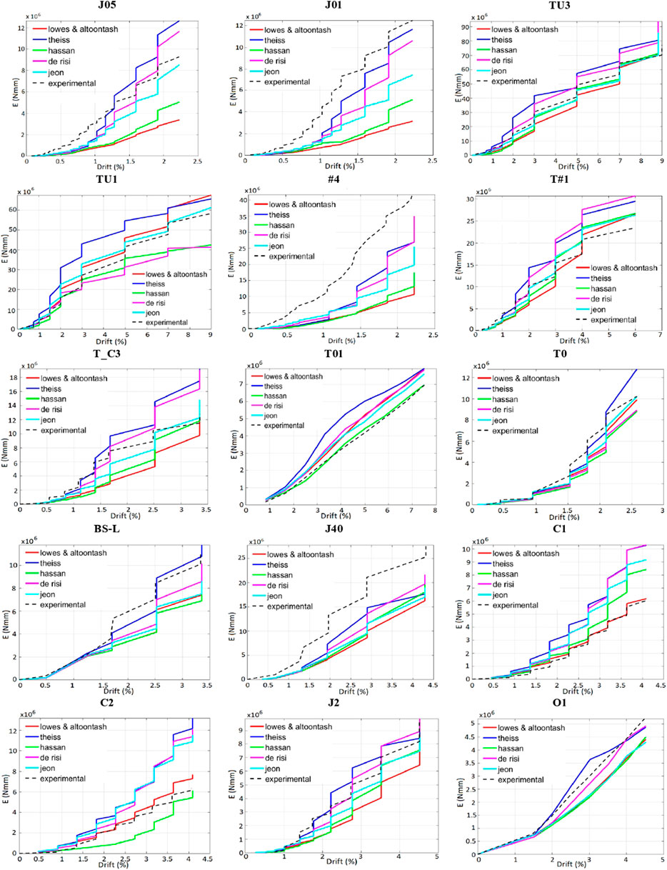
FIGURE 11. Cumulative dissipated energy: comparison among the literature models.
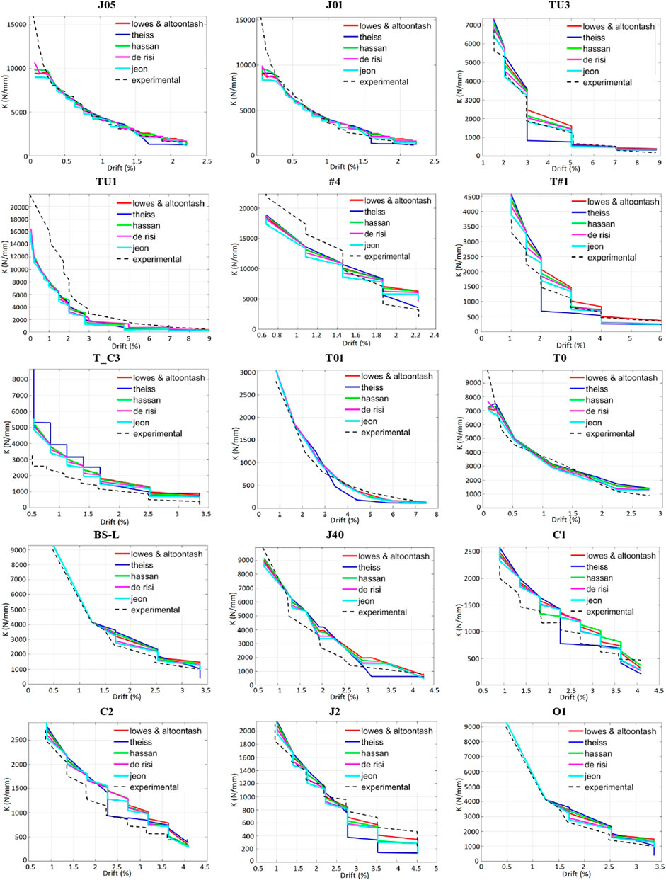
FIGURE 12. Stiffness degradation: comparison among the literature models.
As observed, a large scatter among the considered models is found in terms of numerical energy dissipation (Figure 11), whereas only slight differences are noted in terms of stiffness decay (Figure 12).
As emerged from the outcomes shown in Table 11, the numerical model derived by adopting the pinching parameters proposed by Theiss (2005) provided the less accurate results in terms of dissipated energy and stiffness degradation. Conversely, the best numerical simulations are those generally obtained considering the proposal by Jeon (2013) The good accuracy is also confirmed by analyzing the plots in terms of force – drift hysteretic cycles shown in Figure 13 where the experimental curves are compared to the numerical ones obtained by using the pinching parameters proposed by Jeon (2013) (the cyclic simulations obtained by using the pinching parameters suggested by the other proposals are omitted for the sake of brevity). Of course, in order to further improve the cyclic modelling of the considered RC joints, an ad-hoc calibration procedure of the “pinching4” model parameters should be performed by considering the collected experimental database; to this purpose, a good starting point is represented by the outcomes of the numerical study performed herein, suggesting to focus on the sets of parameters proposed by Jeon (2013) and by De Risi (2015), and opportunely modify them by spanning within the values proposed by these authors. However, this aspect is omitted herein and will be addressed in another paper under preparation.
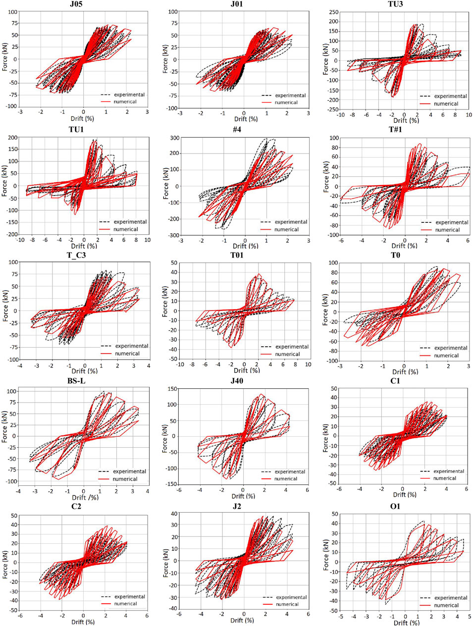
FIGURE 13. Force – drift cyclic response using the pinching parameters proposed by Jeon (Mitra and Lowes, 2007).
Conclusion
Past and recent earthquake events have underlined a behavior of existing RC frame structures in some cases characterized by significant damages and failure of beam-column joints. This unexpected behavior has led to a particular attention of the scientific community toward the assessment, verification and design of this important component of RC frames.
In this study, a numerical modelling approach to evaluate the behavior of exterior RC beam – column joints has been presented. In particular, starting from the outcomes of a previous study carried out by the authors, a calibration process based on a set of experimental tests has been carried out in order to derive an efficient constitutive model for exterior RC joints.
To this end, non-linear static analyses carried out by implementing the scissor model in the software OpenSees have been performed by simulating both the monotonic experimental behavior and the cyclic response of the selected experimental cases.
The monotonic analyses have been preliminary finalized to identify among the models of literature the ones that better simulate the experimental behavior of the selected specimens. From these analyses it has been observed that the model by Kim and LaFave (2009) and the model by Jeon (2013) are the most reliable in predicting the shear strength of the examined joints, while the deformability level is better approximated by the strain parameters proposed by the model by De Risi et al. (2016). Subsequently, the calibration process has been carried out to improve the capacity of the model to simulate the monotonic response of exterior RC joints.
Moreover, cyclic analyses have been carried out considering the model derived from the calibration process here presented and some literature proposals for defining the set of parameters governing the hysteresis rules and pinching effect. The obtained results, although have clearly emphasized the great complexity in simulating the cyclic response, have pointed out the reliability of the proposed model and, also, provided useful indications on how to further improve the cyclic modelling of the considered RC joints.
Data Availability Statement
The raw data supporting the conclusions of this article will be made available by the authors, without undue reservation.
Author Contributions
EG, AN and RN contributed to: Conceptualization, Methodology, Investigation, Validation, Software, Formal analysis, Data curation, Writing-original draft. MI and RR contributed to: Conceptualization, Methodology, Investigation, Resources, Visualization, Writing-review and editing, Supervision, Project administration, Funding acquisition. All authors approved the submitted version.
Funding
Funding received from University of Salerno for open access publication fees.
Conflict of Interest
The authors declare that the research was conducted in the absence of any commercial or financial relationships that could be construed as a potential conflict of interest.
Publisher’s Note
All claims expressed in this article are solely those of the authors and do not necessarily represent those of their affiliated organizations, or those of the publisher, the editors and the reviewers. Any product that may be evaluated in this article, or claim that may be made by its manufacturer, is not guaranteed or endorsed by the publisher.
Acknowledgments
The financial support by ReLUIS (Network of the Italian University Laboratories for Seismic Engineering–Italian Department of Civil Protection) is gratefully acknowledged (Executive Project 2019-21 - WP14/WP2 CARTIS). Further support has been given by University of Salerno (FARB 2020).
References
ACI 369 R-11 (2011). Guide for Seismic Rehabilitation of Existing Concrete Frame Buildings and Commentary. Farmington Hills, MI: American Concrete Institute.
Akguzel, U., and Pampanin, S. (2012). Assessment and Design Procedure for the Seismic Retrofit of Reinforced Concrete Beam-Column Joints Using FRP Composite Materials. J. Compos. Constr. 16 (1), 21–34. doi:10.1061/(ASCE)CC.1943-5614.0000242
Al-Salloum, Y. A., Siddiqui, N. A., Elsanadedy, H. M., Abadel, A. A., and Aqel, M. A. (2011). Textile-reinforced Mortar versus FRP as Strengthening Material for Seismically Deficient RC Beam-Column Joints. J. Compos. Constr. 15, 920–933. doi:10.1061/(asce)cc.1943-5614.0000222
Alath, S., and Kunnath, S. K. (1995). “Modeling Inelastic Shear Deformations in RC Beam–Column Joints,” in Engineering mechanics proceedings of 10th conference 1995. ASCE, New York, May 21-24, 1995 (Boulder, Colorado: University of Colorado at Boulder), 822–825.
Alire, D. A. (2002). “Seismic Evaluation of Existing Unconfined Reinforced Concrete Beam–Column Joints,”M.Sc. Thesis (University of Washington).
Antonopoulos, C. P., and Triantafillou, T. C. (2003). Experimental Investigation of FRP-Strengthened RC Beam-Column Joints. J. Compos. Constr. 7 (1), 39–49. doi:10.1061/(asce)1090-0268(2003)7:1(39)
ASCE/SEI 41/06 (2006). Seismic Rehabilitation of Existing Buildings. Reston, Virginia: American Society of Civil Engineers.
Bedirhanoglu, I., Ilki, A., Pujol, S., and Kumbasar, N. (2010). Behavior of Deficient Joints with plain Bars and Low-Strength concrete. ACI Struct. J. 107, 300–310.
Biddah, A., and Ghobarah, A. (1999). Modelling of Shear Deformation and Bond Slip in Reinforced concrete Joints. Struct. Eng. Mech. 7 (4), 413–432. doi:10.12989/sem.1999.7.4.413
Bousselham, A. (2010). State of Research on Seismic Retrofit of RC Beam-Column Joints with Externally Bonded FRP. J. Compos. Constr. 14, 49–61. doi:10.1061/(asce)cc.1943-5614.0000049
Celik, O. C., and Ellingwood, B. R. (2008). Modeling Beam-Column Joints in Fragility Assessment of Gravity Load Designed Reinforced Concrete Frames. J. Earthquake Eng. 12, 357–381. doi:10.1080/13632460701457215
Clyde, C., Pantelides, C. P., and Reavely, L. D. (2000). “Performance-Based Evaluation of Exterior Reinforced concrete Building Joints for Seismic Excitation,”. PEER report 2000/05 (Berkeley, CA: Pacific Earthquake Engineering Research Center, College of Engineering, University of California).
De Risi, M. T. (2015). “Seismic Performance Assessment of RC Buildings Accounting for Structural and Non-structural Elements,”Ph.D. Thesis (University of Napoli, Federico II).
De Risi, M. T., Ricci, P., and Verderame, G. M. (2016). Modelling Exterior Unreinforced Beam-Column Joints in Seismic Analysis of Non-ductile RC Frames. Earthquake Engng Struct. Dyn. 46 (6), 899–923. doi:10.1002/eqe.2835
De Vita, A., Napoli, A., and Realfonzo, R. (2017). Full Scale Reinforced concrete Beam-Column Joints Strengthened with Steel Reinforced Polymer Systems. Front. Mater. 4, 1–17. doi:10.3389/fmats.2017.00018
Deifalla, A., Ahmed, F., Saleh, A., Elwan, S., Hamad, M., and Elzeiny, S. (2021). Effect of Reinforcement Around Web Opening on the Cyclic Behavior of Exterior RC Beam-Column Joints. Future Eng. J. 2 (1).
Del Vecchio, C., Di Ludovico, M., Balsamo, A., Prota, A., Manfredi, G., and Dolce, M. (2014). Experimental Investigation of Exterior RC Beam-Column Joints Retrofitted with FRP Systems. J. Composites Construction 18 (4), 1–13. doi:10.1061/(ASCE)CC.1943-5614.0000459
El-Amoury, T., and Ghobarah, A. (2002). Seismic Rehabilitation of Beam-Column Joint Using GFRP Sheets. Eng. Structures 24, 1397–1407. doi:10.1016/S0141-0296(02)00081-0
El-Metwally, S. E., and Chen, W. F. (1988). Moment-Rotation Modeling of Reinforced Concrete Beam-Column Connections. ACI Struct. J. 85 (4), 384–394.
Genesio, G. (2012). “Seismic Assessment of RC Exterior Beam-Column Joints and Retrofit with Haunches Using post-installed Anchors,”. Ph.D. thesis (Germany: University of Stuttgart). doi:10.18419/OPUS-472
Giberson, M. F. (1969). Two Nonlinear Beams with Definitions of Ductility. J. Struct. Div.ASCE 95, 137–157. doi:10.1061/jsdeag.0002184
Grande, E., Imbimbo, M., Napoli, A., Nitiffi, R., and Realfonzo, R. (2021). A Macro-Modelling Approach for RC Beam-Column Exterior Joints: First Results on Monotonic Behavior. J. Building Eng. 39, 1–16. doi:10.1016/j.jobe.2021.102202
Hadi, M. N. S., and Tran, T. M. (2016). Seismic Rehabilitation of Reinforced concrete Beam-Column Joints by Bonding with concrete Covers and Wrapping with FRP Composites. Mater. Struct. 49, 467–485. doi:10.1617/s11527-014-0511-4
Haselton, C. B., Liel, A. B., Taylor-Lange, S. C., and Deierlein, G. G. (2016). Calibration of Model to Simulate Response of Reinforced concrete Beam-Columns to Collapse. ACI Struct. J. 113 (6), 1141–1152. doi:10.14359/51689245
Hassan, W., Al-Zahraa Refaie, F., and Belal, A. (2018). “Seismic Vulnerability of concrete Beam-Column Joints in Older Construction under High Axial Loads”. In: Proceeding of the 16th European Conference on earthquake engineering, Thessaloniki, Greece, June 18–21 (Springer), 1–10.
Hassan, W. M. (2011). “Analytical and Experimental Assessment of Seismic Vulnerability of Beam-Column Joints without Transverse Reinforcement in Concrete Buildings,”. Ph.D. Thesis (Berkeley: University of California).
Hwang, S., and Lee, H. (1999). Analytical Model for Predicting Shear Strengths of Exterior Reinforced concrete Beam-Column Joints for Seismic Resistance. ACI Struct. J. 96 (5), 846–857.
Jeon, J.-S., Lowes, L. N., DesRoches, R., and Brilakis, I. (2015). Fragility Curves for Non-ductile Reinforced concrete Frames that Exhibit Different Component Response Mechanisms. Eng. Structures 85, 127–143. doi:10.1016/j.engstruct.2014.12.009
Jeon, J. S. (2013). “Aftershock Vulnerability Assessment of Damaged Reinforced concrete Buildings in California,”. Ph.D. Thesis (GA: School of Civil and Environmental Engineering, Georgia Institute of Technology). doi:10.1061/9780784412848.230
Kim, J., and LaFave, J. M. (2009). “Joint Shear Behavior of Reinforced concrete Beam-Column Connections Subjected to Seismic Lateral Loading,”Report No. NSEL-020 (IL: Department of Civil and Environmental Engineering, University of Illinois at Urbana-Champaign).
Kim, J., and LaFave, J. M. (2012). A Simplified Approach to Joint Shear Behavior Prediction of RC Beam-Column Connections. Earthquake Spectra 28 (3), 1071–1096. doi:10.1193/1.4000064
Liel, A. B., Haselton, C. B., and Deierlein, G. G. (2010). Seismic Collapse Safety of Reinforced concrete Buildings. II: Comparative Assessment of Nonductile and Ductile Moment Frames. J. Struct. Eng. 137 (4), 492–502.
Lowes, L. N., Mitra, N., and Altoontash, A. (2003). A Beam-Column Joint Model for Simulating the Earthquake Response of Reinforced Concrete Frames. University of California. Berkeley: Pacific Earthquake Engineering Research Center.
Lowes, L. N., and Altoontash, A. (2003). Modeling Reinforced-Concrete Beam-Column Joints Subjected to Cyclic Loading. J. Struct. Eng. 129, 1686–1697. doi:10.1061/(asce)0733-9445(2003)129:12(1686)
Mayes, R. L., and Clough, R. W. (1975). “State of the Art in Seismic Shear Strength of Masonry – an Evaluation and Review,”. EERC Report (CA: University of Berkeley).
McKenna, F., Fenves, G. L., and Scott, M. H. (2010). OpenSees: Open System for Earthquake Engineering Simulation, Pacific Earthquake Engineering Research Center. Berkeley, CA, USA: University of California. http://opensees.berkeley.edu.
Mitra, N., and Lowes, L. N. (2007). Evaluation, Calibration, and Verification of a Reinforced Concrete Beam-Column Joint Model. J. Struct. Eng. 133 (1), 105–120. doi:10.1061/(asce)0733-9445(2007)133:1(105)
Otani, S. (1974). Inelastic Analysis of R/C Frame Structures. J. Struct. Division 100, 1433–1449. doi:10.1061/jsdeag.0003821
Pantelides, C. P., Hansen, J., Nadauld, J., and Reavely, L. D. (2002). “Assessment of Reinforced concrete Building Exterior Joints with Substandard Details,”. PEER Report 2002/18 (Berkeley, CA: Pacific Earthquake Engineering Research Center, College of Engineering, University of California).
Park, Y. J., and Ang, A. H. S. (1985). Mechanistic Seismic Damage Model for Reinforced concrete. J. Struct. Eng. 111 (4), 722–739. doi:10.1061/(asce)0733-9445(1985)111:4(722)
Realfonzo, R., Napoli, A., and Pinilla, J. G. R. (2014). Cyclic Behavior of RC Beam-Column Joints Strengthened with FRP Systems. Construction Building Mater. 54, 282–297. doi:10.1016/j.conbuildmat.2013.12.043
Reyes de Ortiz, I. (1993). “Strut-and-Tie Modeling of Reinforced Concrete Short Beams and Beam-Column Joints,”. Ph.D. Thesis (London, United Kingdom: University of Westminster).
Saleh, A., Elwan, S. K., Elzeiny, S., Hamad, M., and Deifalla, A. (2021). Numerical Modeling the Effect of an Opening on the Behavior of Exterior Beam-Column Connections under Cyclic Loading. J. Building Eng. 40, 102742. doi:10.1016/j.jobe.2021.102742
Shafaei, J., Zareian, M. S., Hosseini, A., and Marefat, M. S. (2014). Effects of Joint Flexibility on Lateral Response of Reinforced concrete Frames. Eng. Structures 81, 412–431. doi:10.1016/j.engstruct.2014.09.046
Sharma, A., Eligehausen, R., and Reddy, G. R. (2011). A New Model to Simulate Joint Shear Behavior of Poorly Detailed Beam-Column Connections in RC Structures under Seismic Loads, Part I: Exterior Joints. Eng. Structures 33 (3), 1034–1051. doi:10.1016/j.engstruct.2010.12.026
Shin, M., and LaFave, J. M. (2004). Modeling of Cyclic Joint Shear Deformation Contributions in RC Beam-Column Connections to Overall Frame Behavior. Struct. Eng. Mech. 18 (5), 645–669. doi:10.12989/sem.2004.18.5.645
Stevens, N. J., Uzumeri, S. M., and Collins, M. P. (1991). Reinforced-Concrete Subjected to Reverse-Cyclic Shear – Experiment and Constitutive Model. ACI Struct. J. 88 (2), 135–146.
Theiss, A. G. (2005). “Modeling the Earthquake Response of Older Reinforced Concrete Beam-Column Building Joints,”M.Sc. Thesis (University of Washington).
Tsonos, A. G. (2002). Seismic Repair of Exterior R/C Beam-To-Column Joints Using Two-Sided and Three-Sided Jackets. Struct. Eng. Mech. 13 (1), 17–34. doi:10.12989/sem.2002.13.1.017
Uzumeri, S. M. (1977). “Strength and Ductility of Cast-In-Place Beam-Column Joints,” in American Concrete Institute Annual Convention. Symposium on Reinforced Concrete Structures in Seismic Zones, 293–350.
Vecchio, F. J., and Collins, M. P. (1986). The Modified Compression-Field Theory for Reinforced Concrete Elements Subjected to Shear. ACI J. 83 (2), 219–231.
Vollum, R. L., and Newman, J. B. (1999). Strut and Tie Models for Analysis/design of External Beam-Column Joints. Mag. Concrete Res. 51 (6), 415–425. doi:10.1680/macr.1999.51.6.415
Walker, S. G. (2001). “Seismic Performance of Existing RC Beam–Column Joints,”. M.Sc. Thesis (University of Washington).
Wong, H. F. (2005). “Shear Strength and Seismic Performance of Non-seismically Designed Reinforced concrete Beam-Column Joints,”. Ph.D. Thesis (The Hong Kong University of Science and Technology, Department of Civil Engineering). doi:10.14711/thesis-b914043
Youssef, M., and Ghobarah, A. (2001). Modelling of RC Beam-Column Joints and Structural walls. J. Earthquake Eng. 5 (1), 93–111. doi:10.1080/13632460109350387
Glossary
The symbols used within the paper are reported herein:
A (mm2) joint cross-section area
As,b (mm2) area of the beam longitudinal reinforcement in tension
As,c (mm2) total area of the column longitudinal reinforcement
BI (-) beam reinforcement index equal to (As,b·fyb)/(bb·hb·fc)
D+max,i (mm) displacement corresponding to F+max,i
D-max,i (mm) displacement corresponding to F−max,i (kN)
Ei (N mm) accumulated hysteretic energy at the ith displacement increment
Emonotonic (N mm) energy required to achieve under monotonic loading the deformation that defines failure
Ed,iexp (N mm) experimental dissipated energy calculated at the i-th displacement cycle
Ed,inum (N mm) numerical dissipated energy calculated at the i-th displacement cycle
Err,En (%) mean absolute percentage error calculated on the dissipated energy parameter
Err,F [%] mean absolute percentage error calculated on the force parameter
Err,K (%) mean absolute percentage error calculated on the stiffness degradation parameter
Err,τ (%) mean absolute percentage error calculated on the shear strength parameter
Fexp,i (kN) ith value of the experimental force
F+max,i (kN) peak lateral force applied to the beam in the push loading direction at the ith displacement cycle
F−max,i (kN) peak lateral force applied to the beam in the pull loading direction at the ith displacement cycle
Fnum,i (kN) ith value of the numerical force
Ki (N/mm) stiffness loss at ith displacement cycle
Kiexp(N/mm) experimental stiffness calculated at the i-th displacement cycle
Kinum(N/mm) numerical stiffness calculated at the i-th displacement cycle
Lb (mm) beam length
Lc (mm) column length
M (kN m) generic bending moment corresponding to the joint shear stress
Mj (kN m) jth bending moment corresponding to the jth shear stress τj
M1s (kN mm) bending moment at beam cracking associated to the slip s1
M2s (kN mm) bending moment at pre-peak phase associated to the slip s2
M3s (= Mmaxs) (kN m) maximum bending moment associated to the slip s3
M4s (kN m) residual bending capacity associated to the slip s4
N (N) axial force applied to the column
Tb (N) tensile force acting in the beam longitudinal bars
Vcol (N) column shear force
Xj (-) jth predictor (independent) variable
Y (-) response (dependent) variable
ab (mm) depth of the neutral axis in the beam, evaluated assuming plane section
bb (mm) width of the beam cross-section
bc (mm) width of the column cross-section
bj (mm) effective joint width, equal to bj = minbc; (bc + bb/2]
d-d′ (mm) distance between the longitudinal reinforcements in tension and compression of the beam
dmax (mm) maximum historic deformation demands
dmin (mm) minimum historic deformation demands
dmax,i (mm) current deformation defining the end of the reload cycle for increasing deformation demand
dmax,0 (mm) maximum (or minimum) historic deformation demand
defmax (mm) positive deformations that define failure
defmin (mm) negative deformations that define failure
fc (MPa) cylinder compressive strength of concrete
fmax,i (kN) current envelope maximum strength
fmax,0 (kN) initial envelope maximum strength for the case of no damage
fstm,tr (MPa) mean value of the maximum tensile stress developed in the bar that can be transferred by bond
fst,0 (MPa) maximum bond stress estimated in absence of confining effect
fyb (MPa) steel yield strength of beam reinforcement
fyc (MPa) steel yield strength of column reinforcement;
gE (-) multiplication factor used to define the maximum energy dissipation under cyclic loading
ki (N/mm) current unloading stiffness
k0 (N/mm) k0 is the initial unloading stiffness for the case of no damage
hb (mm) height of the beam cross-section
hc (mm) height of the column cross-section
jdb (mm) beam internal lever arm
lb (mm) anchorage length of the longitudinal bar (the bond stress is assumed uniform over this length)
m (-) number of available measures
n (-) total number of measures considered in the analysis
ptr (MPa) the transverse pressure in the column (equal to σj)
s (mm) slip of the beam’s reinforcing bars under tension
s1 (mm) slip s associated to the bending moment at beam crackingM1s
s2 (mm) slip s associated to the bending moment at pre-peak phase M2s
s3 (mm) slip s associated to the maximum bending moment M3s
s4 (mm) slip s associated to the residual bending capacity M4s
θ (mm) longitudinal bar diameter;
αj (-) jth parameter required to fit the damage rule to experimental data
βj (-) coefficient of the regression analysis
γ (-) generic shear strain value
γj (-) jth joint shear strain
γ1 (-) shear strain corresponding to τ1
γ2 (-) shear strain corresponding to τ2
γ3 (-) shear strain corresponding to τ3 = τmax
γ4 (-) shear strain corresponding to τ4
δi (-) damage index at the ith displacement increment (0 in case of no damage, 1 in case of maximum damage)
δlim (-) maximum possible value of the damage index
δdi (-) current value of the reloading – strength damage index
δfi (-) current value of the strength damage index
δki (-) current value of the stiffness damage index
θ (rad) generic rotation corresponding to the joint shear strain
θj (rad) jth joint rotation
θs (rad) joint rotation due to slip of the beam’s reinforcing bars under tension
λ (-) parameter accounting for the bending shape of the beam’s longitudinal steel bar end inside the joint (λ = 1.0 in the case of a “L-shape” configuration; λ = 0.9 in the case of a “U-shape” one)
σj (MPa) ratio between the column axial load (N) and the corresponding cross-section area bc∙hc of the column
τ (MPa) generic shear stress value
τj (MPa) jth joint shear stress
τ1 (MPa) shear stress at joint craking
τ2 (MPa) shear stress at pre-peak phase
τ3 (= τmax) (MPa) shear stress at peak
τ4 (MPa) residual shear strength
φ angle between the strut and the longitudinal beam axis
Keywords: RC beam-column joints, shear capacity, numerical non-linear analysis, cyclic loading, pinching parameters, OpenSees code, experimental vs numerical comparison
Citation: Grande E, Imbimbo M, Napoli A, Nitiffi R and Realfonzo R (2021) A Nonlinear Macro-Model for the Analysis of Monotonic and Cyclic Behaviour of Exterior RC Beam-Column Joints. Front. Mater. 8:719716. doi: 10.3389/fmats.2021.719716
Received: 02 June 2021; Accepted: 12 July 2021;
Published: 29 July 2021.
Edited by:
Libo Yan, Fraunhofer Institute for Wood Research, GermanyCopyright © 2021 Grande, Imbimbo, Napoli, Nitiffi and Realfonzo. This is an open-access article distributed under the terms of the Creative Commons Attribution License (CC BY). The use, distribution or reproduction in other forums is permitted, provided the original author(s) and the copyright owner(s) are credited and that the original publication in this journal is cited, in accordance with accepted academic practice. No use, distribution or reproduction is permitted which does not comply with these terms.
*Correspondence: Annalisa Napoli, annapoli@unisa.it