 Matthew P. Shortell
 Marwan A. M. Althomali
 Marie-Luise Wille
 Christian M. Langton
- 1Science and Engineering Faculty, Institute of Health and Biomedical Innovation, Queensland University of Technology, Brisbane, QLD, Australia
- 2University College in Al-Jamoum, Umm Al-Qura University, Mecca, Saudi Arabia
- 3Laboratory of Ultrasonic Electronics, Doshisha University, Kyotanabe, Japan
We demonstrate a simple technique for quantitative ultrasound imaging of the cortical shell of long-bone replicas. Traditional ultrasound computed tomography instruments use the transmitted or reflected waves for separate reconstructions but suffer from strong refraction artifacts in highly heterogeneous samples such as bones in soft tissue. The technique described here simplifies the long bone to a two-component composite and uses both the transmitted and reflected waves for reconstructions, allowing the speed of sound and thickness of the cortical shell to be calculated accurately. The technique is simple to implement, computationally inexpensive, and sample positioning errors are minimal.
Introduction
X-ray-based modalities are currently used as the primary method to determine bone health (Genant et al., 1996; Barkmann and Glüer, 2011). Unfortunately, they are far from perfect at predicting the mechanical properties and regular testing of patients cannot be performed due to limits on X-ray exposure levels. Over the past three decades, quantitative ultrasound methods have been heavily investigated for quantifying bone health due to the inherent relationship between ultrasound waves and mechanical properties of materials (Langton et al., 1984; Laugier and Haïat, 2011; Raum et al., 2014).
One of the earliest demonstrations of a portable clinical quantitative ultrasound system to determine bone ultrasound properties was the CUBA system (Langton et al., 1990) which measured the broadband ultrasound attenuation (BUA) and speed of sound (SOS) through ultrasound transmission measurements. However, for long bones, most recent efforts have focused on single-sided pulse-echo techniques to determine the cortical shell thickness and SOS (Foldes et al., 1995; Sievänen et al., 2001; Chen et al., 2004). These instruments require a highly trained operator to make decisions on how and where to place the transducers on the skin, making them inherently operator dependent. A computed tomography (CT)-based quantitative ultrasound approach for long bones would not require a highly trained operator, would be highly repeatable, and provide 3D detailed spatial information to the clinician as well.
There has been a plethora of research into quantitative ultrasound computed tomography (UCT) for soft tissues for applications such as detecting cancer risk in breast tissue (André et al., 2013). In these soft tissues, refraction artifacts have a small but significant effect on reconstructed images. Several image reconstruction methods have been developed to overcome this small perturbation from the straight ray approximation. Unfortunately, using these techniques in highly heterogeneous media such as bone in soft tissue is not possible (Lasaygues et al., 2010).
Typically, there are two types of UCT techniques: transmission UCT (T-UCT) and pulse-echo UCT (PE-UCT). T-UCT uses a similar principle to traditional X-ray CT by measuring the ultrasound pulse transmitted through the sample at different rotation angles and translational positions. In soft tissue, this can produce accurate high-resolution quantitative maps of BUA and SOS in the tissue. In samples containing bone, the images are not quantitative and produce a blurry image of the bone; the cortical thickness cannot be accurately measured.
Pulse-echo UCT methods are usually defined as non-quantitative; they usually cannot provide a SOS map of the bone. They can produce high-resolution images of the outer bone surface. To determine the structure of the inner cortical shell surface, a bone SOS value based on previous ex vivo ultrasound transmission measurements of a population is used. Since bone SOS is an indicator of bone health as well as cortical shell thickness, the reconstruction of the shell inner surface is unreliable using this technique.
The Lasaygues group has led the way in extending UCT to allow quantitative imaging of the long-bone cortical shell with two main methods developed. Compound Quantitative Ultrasonic Tomography (CQUT) is an iterative experimental method that compensates for refraction by adjusting the transmitting and receiving transducer locations and angles to sample the equivalent straight path through the bone (Lasaygues, 2007). Distorted Born Diffraction Tomography (DBDT) uses a single set of experiments but performs iterative simulations of the sample (Lasaygues et al., 2006). Although both CQUT and DBDT have resulted in good quantitative images of the cortical shell, they require either multiple experiments and heavy data processing requirements (CQUT) or are very computationally time expensive (DBDT). A fast and simple technique for quantitative UCT of long bones to output the key clinically relevant metrics has not been developed yet.
Here, we demonstrate a simple and fast UCT technique (PE-T-UCT) to extract an average bone SOS and a mean cortical shell thickness. The useful data in T-UCT are combined with the reconstructed PE image using a two-component model of the cortical shell. We then used this averaged SOS to accurately reconstruct each PE image, avoiding the use of a population averaged SOS.
Theory
Measuring bone SOS and cortical shell thickness using transmitted and reflected pulses has been proposed by Zheng and Lasaygues (2013) using single-element transducers at a single angle. It is extended here using reconstructed PE-UCT and T-UCT data instead of the raw echo data. We also use multi-element transducers so that positioning errors are minimal and a better sample average is obtained. For a simple two-component model of cortical bone, the SOS in the bone cortical shell (vb) is assumed to be a constant and all other volumes are assumed to have the SOS in water (vw = 1,483 m/s). The apparent delay time (Δt) of an ultrasound wave travelling through the bone is measured directly in T-UCT. It is calculated as the time taken for the ultrasound wave to pass through the sample minus the time through a reference measurement (water only). It is related to vb by
Here, d is not the bone diameter, but rather the total length of bone that the ultrasound wave propagates through to be detected at the receiving transducer. If we only consider propagation through the middle of the bone, then d is given by the addition of the bone shell thickness on both sides (T1, T2) that the wave propagates through
where t1 and t2 are the time taken for the wave to propagate through the first and second sides of the bone shell, respectively. These equations can be solved to find the SOS in bone as
Although t1 and t2 can be measured directly in a PE sonogram, it is more intuitive to use the reconstructed PE-UCT image. This is particularly important in complex samples where different transducer positions are required to resolve the inner and outer interfaces. In the PE-UCT reconstruction, the SOS is assumed to be vw everywhere, causing the shell thickness to appear thinner in a PE-UCT image. This reduced thickness ( or ) can be converted back into a shell propagation time using
Combining Equations (3) and (4) allows the calculation of vb for various angles of sample rotation. The true cortical shell thickness uses the calculated vb values along with the measured apparent thickness values to calculate the corrected thickness values:
Experimental Methods
Data Acquisition
The samples were scanned using a lab-built UCT system (Althomali et al., 2017a,b). Two 2.25-MHz 128-element linear phased-array transducers (Olympus, Corporation, Shinjuku, Tokyo, Japan) were used with an element width of 0.75 mm (xy-plane) and height of 12 mm (z-axis). The total transducer width was therefore 128 × 0.75 = 96 mm. One transducer acted as a transmitter and receiver (for PE-UCT), and the other as a receiver only (for T-UCT). They were coaxially aligned in a fixture 137 mm apart and immersed in a water tank with the sample placed roughly in the center between the two transducers. To obtain a 360° ultrasound scan (in 1° steps), the phased-array transducers were rotated around the z-axis using a user-programmed Motoman HP6 robotic arm (YASKAWA Electric Corporation, Japan). Each transducer was connected to an Omniscan MX device (Olympus, Corporation, Shinjuku, Tokyo, Japan), and controlled by the Olympus TomoView software (version 2.7, Olympus, Corporation, Shinjuku, Tokyo, Japan), to emit and receive the ultrasound signals. Figure 1 shows a schematic representation of the UCT system.
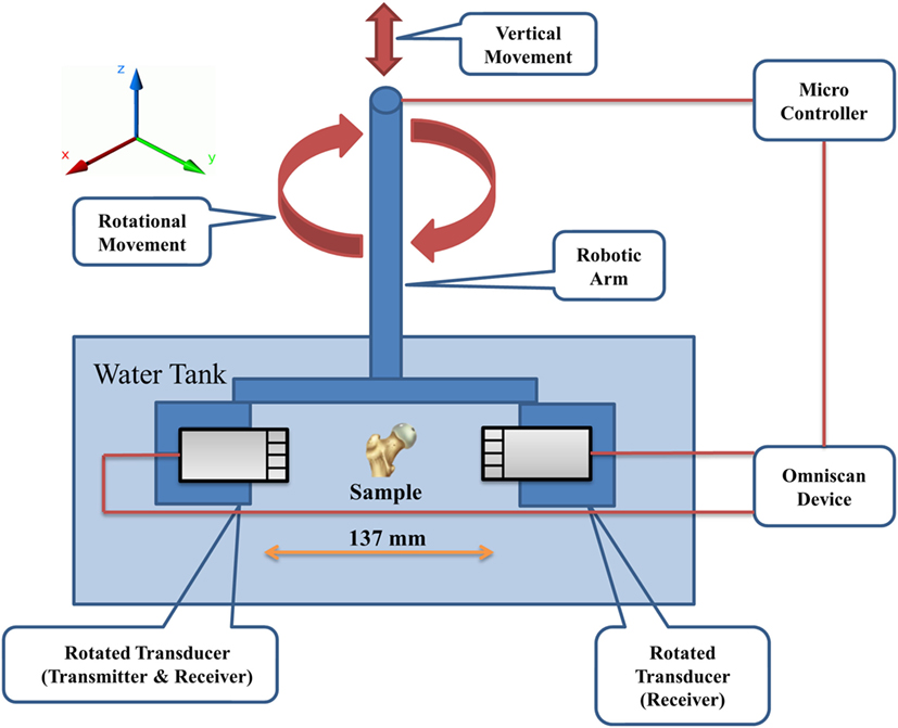
Figure 1. Schematic representation of the UCT system. The robotic arm is used to position the transducers such that the sample is approximately centered between the transducers in the xy-plane and positioned at the correct z-position for imaging. The robotic arm also rotates the transducers during acquisition. UCT, ultrasound computed tomography.
TomoView was used to set all signal acquisition parameters as well as the beam profile. The transmitting transducer was set to fire five neighboring elements at a time (equivalent emitter size of 3.75 mm). These set of five elements were incremented by one for successive scans to give a total of 124 measurements per rotation angle per transducer. The transmitting transducer received data only on the central firing element. The receive-only transducer was set to receive on the same element number directly opposite. Ideally, this results in both transducers only sampling 124 straight paths perpendicular to the transducers. The electronic gain on each transducer was set dynamically depending on the sample to minimize saturation but still resolve all the sample features. The digitization frequency was 25 MHz and the pulse length was 300 ns.
Samples
A simple hollow cylinder structure was studied first to demonstrate the PE-T-UCT concept. Two hollow Perspex cylinders were used with outer diameters of 25 and 35 mm and labeled as P25 and P35, respectively. The holes were drilled as close as possible to the center and the thickness of the shell was approximately 7.5 mm. Although these do not represent real bones, they are simple test cases for demonstrating the PE-T-UCT concept and they have no variation in the z-direction, and hence there are minimal slice averaging effects.
To demonstrate the concept with long bone like shapes, a plastic femur bone from 3B Scientific was used. Three plastic-bone segments each approximately 30 mm long were cut. Holes were drilled through the center of each segment and allowed to fill with water in UCT experiments to mimic the medullary cavity. One sample (PB1) was taken from the Metaphysis and two (PB2 and PB3) were taken from the Diaphysis. Figure 2 shows a photograph of the samples.
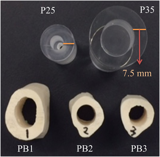
Figure 2. Photograph of the Perspex cylinder samples: P25 and P35 with 25 and 35 mm diameters, respectively, and the plastic-bone samples: PB1, PB2, and PB3.
PE-UCT Reconstructions and Reduced Thickness Calculations
Pulse-echo UCT reconstructions were performed using the fully rectified data collected from the transmitting transducer. Time since transducer firing (τ) was converted into a distance perpendicular to the emitting transducer () using
Using the element position on the transducer () and the rotation angle, the location that the signal originated from can be calculated in the stationary frame (x, y). Each signal from a total of 124 × 360 = 44,640 scans were then binned onto a common xy grid (square pixel size of 0.375 mm) and summed.
ImageJ was used to remove reconstructed interfaces originating from reflections from the sample interfaces on the far side of the sample. These reflections appear much closer to the center of the samples due to the higher velocity experienced through the first side of the sample. They are easily identified by reconstructing only the first half of the data to give a one-sided view of the sample. For the Perspex samples, the inner and outer interfaces were identified using the “findpeaks” function in MATLAB (release 2016b, The MathWorks, Inc., Natick, MA, USA) in a fully automated fashion. For the plastic-bone samples, identification of the interfaces was required by manually drawing a polygon of the inner and outer interfaces over the reconstructed images and thresholding. The apparent shell thickness ( or ) as a function of rotation angle (θ) was found by rotating the image by θ, finding the center of the bone on the -axis and taking the average thickness along the -direction over a width of 1.875 mm. Samples were taken over 360° in 1° steps to compare with the transmission data.
Calculating Apparent Delay Time from Transmission Data
The apparent delay time for each element at each θ is found as the difference in time of arrival (using the maximum of the fully rectified data) of the ultrasound pulse at the receiver compared with when there is no sample present (water only). For samples with an SOS higher than water, this results in a negative Δt if the path length of the received sample is equal to the path length in water. For each θ, only Δt that satisfy μs are used. These bounds were chosen to remove physically unrealistic data that can occur when the signal strength is below the noise level. If there are no elements for an angle that satisfy these criteria, the angle is not used for further calculations and the corresponding and calculated earlier are also removed from further calculations. From the allowed Δt values, the middle (spatially along the transducer) third elements are used to calculate a mean value of Δt for each allowable angle.
SOS and Thickness Calculations
The set of calculated Δt, and values are then used to calculate a set of vb values using Equations (3) and (4). If any of the vb values are outside the bounds of 1,500 < vb < 5,000 m/s then they are excluded along with the corresponding and values. From these allowed vb, and values, the corrected thickness values are then calculated from Equation (5). Average values of the bone SOS () and shell thickness () are then calculated. For visualization of the cortical shell in the PE-T-UCT image, is used to reconstruct the inner interface of the cortical shell along with the existing outer shell from the PE-UCT reconstruction.
Reference Measurements
Speed of sound measurements of the bulk materials were taken with the same experimental apparatus except the transducers remained stationary. For Perspex SOS measurements, a large rectangular Perspex prism was positioned with its largest faces parallel to the transducers; the path length was 24 mm. For plastic bone, an 8 mm thick slice of the femur was cut and positioned with the cut sides parallel to the transducers. In both materials, an average Δt was taken over the middle half of the samples and the was calculated using Equation 1.
To determine the actual shell thickness of the samples, optical images of the samples in the xy-plane from one side were taken using a desktop optical scanner. Thresholding in ImageJ was used to produce binary images of the sample cross-sections for comparison with UCT images and to calculate the average cortical shell thickness. For plastic bone 1, the side closest to the middle of the shaft was used. For the plastic-bone samples, there are slight changes in morphology across the length of the cut samples so the images and derived shell thickness are not as accurate as the Perspex samples.
T-UCT Bulk Attenuation Map Reconstruction
Bulk attenuation (β) maps were reconstructed from the fully rectified transmission data using MATLAB. The ultrasound pulse amplitude through the sample (Is) for each element and angle is compared with the amplitude through water alone (I0) to calculate β using
This produces a 124 × 360 element matrix representing the 124-transducer element locations in the rotating frame and 360 rotations. A 5-point image median filter was then applied to reduce the noise level using the “med2filt” function. Image reconstruction was then performed using the inverse radon transformation (“iradon” function) with linear interpolation and Ram-Lak filter. Finally, a 33% threshold was applied to the reconstructed image for clarity. Reconstructions using the metrics of BUA and SOS were also attempted. Unfortunately, the data were too noisy for BUA calculations and the SOS reconstruction was nonsensical in most samples.
Results and Discussion
Strong refraction and reflection in the transition of ultrasound waves between soft tissue and bone have a detrimental effect in T-UCT. Figure 3 shows the received ultrasound signal across the elements after propagating through the 35 mm hollow Perspex cylinder. Since the SOS in Perspex is higher than water, there should be a negative time delay seen at the receiving transducers in the absence of refraction. Through the center of the cylinder where the curvature is at a minimum this does occur and the delay time would be correctly calculated for image reconstruction. As we look further from the center, the delay time increases toward zero even though the bone projection should appear thicker away from the center. This is due to refraction; the path length is increasing and offsetting the higher SOS in the Perspex. Far from the center, there is a positive delay time due to the very high reflection of most the incident plane wave. The only part of the wave that is detected by the receiving transducer element has gone through such large refraction angles that the path length has increased greatly. This phenomenon makes it impossible to reconstruct high-resolution qualitative (let alone quantitative) reconstructions of bone in T-UCT without using more complicated methods (Lasaygues et al., 2010).
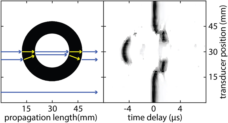
Figure 3. Schematic representation of ultrasound propagation through a hollow 35 mm diameter Perspex cylinder (left) and the resulting ultrasound signal amplitude detected at the receiving transducer as a function of time (right). As each wave propagates from the transmitting transducer, it experiences different propagation speeds when it travels through different media. Each wave can also experience different path lengths if there is significant refraction occurring. The combination of both effects results in a time delay registered at the receiving transducer compared with propagation through water alone. Each transducer element signal is normalized to the maximum value separately for clarity.
Figure 4 shows cross-sections of the samples studied and reconstructed UCT images. The PE-UCT images generally represent the outside of the samples quite well except for PB1 where the overall size looks the same but the surface shape looks different. This could be because we probed the middle of the sample in UCT but used the end of the sample for reference images. For the other samples, this is not as much a problem since their morphology does not change drastically over the sample height like PB1. The T-UCT images give a blurred image of the sample cross-sections. In general, the size appears contracted but also broadened resulting in smaller and denser images. The PE-T-UCT reconstructions improved the inner surface of the PE-UCT images greatly. This is most noticeable in PB2 and PB3 samples where the hole has almost returned to being perfectly circular.
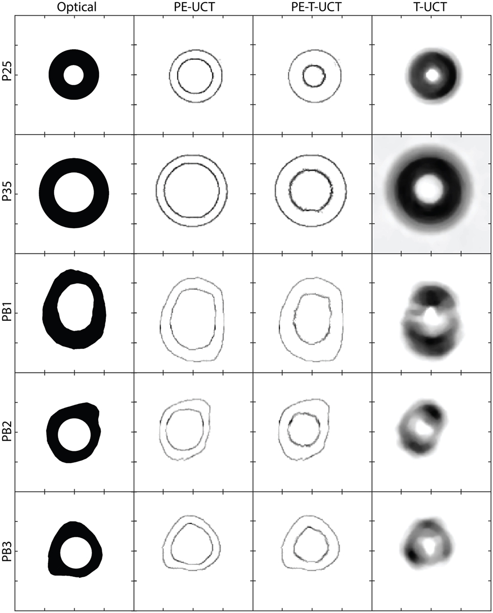
Figure 4. From left to right: the sample dimensions from optical micrographs, PE-UCT reconstructions, PE-T-UCT reconstruction, and T-UCT reconstruction. From top to bottom: P25, P35, PB1, PB2, and PB3. The scale is the same for all images which are 60 mm × 60 mm in size and the tick marks are 15 mm apart. PE-UCT, pulse-echo ultrasound computed tomography; T-UCT, transmission ultrasound computed tomography.
To gain a quantitative understanding of how well the UCT system performed, Table 1 shows the calculated bone outer diameter, SOS, and bone thickness, as well as the reference measurements values. First, we calculate the average sample outer diameter () to see how well the PE-UCT system is working. The PE-UCT system performed quite well considering it is a lab-built system. The diameters measured for P25 and P35 suggest that there may be a slight center of rotation offset error in the system as they both have a positive error value. These values suggest that the best accuracy of the PE-UCT system is approximately 0.5 mm for measuring the bone diameter. Although this is a large value compared with the thickness of the samples, this error will have little effect on the bone thickness measurement and SOS since the same offset will apply to the inner diameter of the bone. In the P25 and P35 samples, the samples have a perfectly circular cross-section, and therefore the SD (σ) in the actual diameters is near 0. Therefore, the PE-UCT SD in P25 and P35 samples (~0.2 mm) indicates the precision of the PE-UCT system.
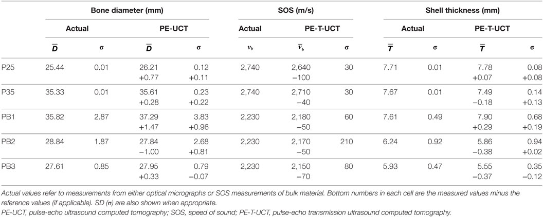
Table 1. Tabulated results of the PE-UCT measured mean bone diameter and PE-T-UCT measured mean SOS and mean shell thickness.
The results for PB1-3 are, as expected, not as good as the ideal Perspex samples. This is in part due to the inaccuracy of the reference measurements, but also due to the increased noise in the rougher plastic-bone samples. Given the larger distribution of diameter sizes in the plastic bones, the largest error of less than 4% is still quite reasonable for a lab-built system.
The SOS measurements for the bulk materials compared with the mean SOS from PE-T-UCT reconstructions are shown next. The SOS is consistently slightly underestimated with a maximum error of <5%. The SD is not sufficiently high to suggest that it is a noise issue in the measurement technique. It is likely that the underestimation of the sample velocity is due to refraction in the samples causing, on average, a slightly longer path length and hence a slightly lower delay time in the transmission measurements.
Since both the Perspex and plastic-bone samples are made of a single homogeneous material, the SOS SD represents the precision of the method. For the simple Perspex samples the precision is very high at 30 m/s, while for the more complex bone samples it is closer to 100 m/s.
The average measured shell thickness is shown in Table 1 with their SD for both optical micrograph and PE-T-UCT measurements. Despite the slight underestimation in SOS values from PE-T-UCT, there is no clear overestimation in the thickness values, although the sample size is limited. All the Perspex and plastic-bone samples are within 3 and 7% of the optical micrograph measurements, respectively. The Perspex samples have holes that are well centered, and hence the SD in the optical micrograph shell thickness is very small. The SD in the PE-T-UCT results suggests that the best possible precision for bone thickness is near 0.1 mm for the PE-T-UCT technique with the UCT setup used. The bone thickness varies considerably in the plastic-bone samples which is adequately represented in the PE-T-UCT results.
Conclusion and Future Work
We have demonstrated a simple UCT method (PE-T-UCT) to measure the cortical shell thickness and the SOS in the cortical shell of long-bone replicas. Although it uses standard phased-array transducers, it can easily be implemented from standard B-scan ultrasound systems or from commercial UCT breast imaging systems using rotating phased-array transducers. The technique is computationally inexpensive and sample positioning errors are minimal since a trained operator is not required to position transducers.
This technique has several avenues for extension and improved accuracy. A more accurate estimate of the path length through the bone would help obtain more accurate SOS measurements. Given the simple two-component model considered, this could potentially be done through ray-tracing simulations to keep the post-processing time short. This would need to be an iterative procedure since the SOS in bone would be unknown. However, the number of iterations would be minimal given the start points are within 5% of the actual SOS and within 10% of the cortical shell thickness.
Author Contributions
MS contributed to the design of the UCT system for PE-UCT and T-UCT, carried out the experiments, performed the data analysis, and wrote the manuscript. MA prepared all the samples and performed the experiments. M-L W wrote the manuscript. CL contributed to the design of the experiment and writing of the manuscript.
Conflict of Interest Statement
The authors declare that the research was conducted in the absence of any commercial or financial relationships that could be construed as a potential conflict of interest.
References
Althomali, M. A., Wille, M.-L., Shortell, M. P., Epari, D. R., Koponen, J., Johnston, M., et al. (2017a). Estimation of Mechanical Stiffness by Finite Element Analysis of Ultrasound Computed Tomography (UCT-FEA); A Comparison with Conventional FEA in Simplistic Structures.
Althomali, M. A. M., Wille, M.-L., Shortell, M. P., and Langton, C. M. (2017b). Estimation of Mechanical Stiffness by Finite Element Analysis of Ultrasound Computed Tomography (UCT-FEA); A Comparison with microCT Based FEA in Cancellous Bone Replica Models.
André, M., Wiskin, J., and Borup, D. (2013). Quantitative Ultrasound in Soft Tissues (Dordrecht: Springer). doi: 10.1007/978-94-007-6952-6
Barkmann, R., and Glüer, C.-C. (2011). “Clinical applications,” in Bone Quantitative Ultrasound, eds P. Laugier, and G. Haïat (Dordrecht: Springer Netherlands), 73–81.
Chen, T., Chen, P.-J., Fung, C.-S., Lin, C.-J., and Yao, W.-J. (2004). Quantitative assessment of osteoporosis from the tibia shaft by ultrasound techniques. Med. Eng. Phys. 26, 141–145. doi:10.1016/j.medengphy.2003.09.001
Foldes, A. J., Rimon, A., Keinan, D. D., and Popovtzer, M. M. (1995). Quantitative ultrasound of the tibia: a novel approach for assessment of bone status. Bone 17, 363–367. doi:10.1016/S8756-3282(95)00244-8
Genant, H. K., Engelke, K., Fuerst, T., Glüer, C.-C., Grampp, S., Harris, S. T., et al. (1996). Noninvasive assessment of bone mineral and structure: state of the art. J. Bone Miner. Res. 11, 707–730. doi:10.1002/jbmr.5650110602
Langton, C. M., Ali, A. V., Riggs, C. M., Evans, G. P., and Bonfield, W. (1990). A contact method for the assessment of ultrasonic velocity and broadband attenuation in cortical and cancellous bone. Clin. Phys. Physiol. Meas. 11, 243–249. doi:10.1088/0143-0815/11/3/007
Langton, C. M., Palmer, S. B., and Porter, R. W. (1984). The measurement of broadband ultrasonic attenuation in cancellous bone. Eng. Med. 13, 89–91. doi:10.1243/EMED_JOUR_1984_013_022_02
Lasaygues, P. (2007). Compound quantitative ultrasonic tomography of long bones using wavelets analysis. Acoust. Imag. 28, 223–229. doi:10.1007/1-4020-5721-0_24
Lasaygues, P., Guillermin, R., and Lefebvre, J.-P. (2006). Distorted born diffraction tomography applied to inverting ultrasonic field scattered by noncircular infinite elastic tube. Ultrason. Imaging 28, 211–229. doi:10.1177/016173460602800402
Lasaygues, P., Guillermin, R., and Lefebvre, J.-P. (2010). “Ultrasonic computed tomography,” in Bone Quantitative Ultrasound, eds P. Laugier, and G. Haïat (Dordrecht: Springer Netherlands), 441–459.
Laugier, P., and Haïat, G. (eds). (2011). “Introduction to the physics of ultrasound,” in Bone Quantitative Ultrasound (Dordrecht: Springer Netherlands), 29–45.
Raum, K., Grimal, Q., Varga, P., Barkmann, R., Glüer, C. C., and Laugier, P. (2014). Ultrasound to assess bone quality. Curr. Osteoporos. Rep. 12, 154–162. doi:10.1007/s11914-014-0205-4
Sievänen, H., Cheng, S., Ollikainen, S., and Uusi-Rasi, K. (2001). Ultrasound velocity and cortical bone characteristics in vivo. Osteoporos. Int. 12, 399–405. doi:10.1007/s001980170109
Keywords: ultrasound, computed tomography, long bones, bone thickness, bone velocity
Citation: Shortell MP, Althomali MAM, Wille M-L and Langton CM (2017) Combining Ultrasound Pulse-Echo and Transmission Computed Tomography for Quantitative Imaging the Cortical Shell of Long-Bone Replicas. Front. Mater. 4:40. doi: 10.3389/fmats.2017.00040
Received: 24 August 2017; Accepted: 09 November 2017;
Published: 29 November 2017
Edited by:
Gianluca Tozzi, University of Portsmouth, United KingdomReviewed by:
Pasquale Vena, Politecnico di Milano, ItalyMarco Miniaci, UMR6294 Laboratoire Ondes et Milieux Complexes (LOMC), France
Copyright: © 2017 Shortell, Althomali, Wille and Langton. This is an open-access article distributed under the terms of the Creative Commons Attribution License (CC BY). The use, distribution or reproduction in other forums is permitted, provided the original author(s) or licensor are credited and that the original publication in this journal is cited, in accordance with accepted academic practice. No use, distribution or reproduction is permitted which does not comply with these terms.
*Correspondence: Christian M. Langton, Y2hyaXN0aWFuLmxhbmd0b25AcXV0LmVkdS5hdQ==