Spatiotemporal variation characteristics and forecasting of the sea surface temperature in the North Indian Ocean

Sea surface temperature (SST) is important for marine environment, and the variation of SST in the North Indian Ocean (NIO) might influence the climate in the local and surrounding area significantly. The empirical orthogonal function (EOF) was used to analyze the spatiotemporal variation characteristics of SST in the NIO. Simultaneously, seven hydrometeorological elements, including 10-m zonal wind (U10), 10-m meridional wind (V10), SST, 2-m dew-point temperature (D2M), 2-m air temperature (T2M), mean sea level pressure (MSLP), and total cloud cover (TCC), were selected as input factors to construct a daily SST forecast model based on deep learning method with convolutional neural networks (CNN). A linear and unsaturated Relu function was used in this model as activation function, which could overcome vanishing gradients and accelerate training speed. The results indicate that the annual mean SST in the NIO exhibits an increasing trend from 1980 to 2021 with a spatial gradual increase from northwest to southeast. The EOF analysis shows that the first mode contributes 28.4% of the variance, exhibiting a basin-wide uniform warming pattern over the Indian Ocean. Contribution of the second mode is 10.1%, displaying the characteristic zonal dipole pattern of the Indian Ocean Dipole (IOD). Additionally, the SST in the NIO is positively correlated with D2M, T2M, and TCC, while exhibits a negative correlation with MSLP. The correlations with U10 and V10 exhibit significant spatial variability. The constructed SST forecast model has a small prediction error, which is basically stable between ±1°C, and does not exceed 0.5°C in most of the NIO. In spite that the overall prediction error increases with the increase of prediction days, the increase of error is smooth, indicating that the forecast model has a good stability. The SST prediction results preserved the contour and distribution characteristics of the actual images holistically, and the spatiotemporal variation patterns are identical to those of the NIO.

1 Introduction

Sea surface temperature (SST) is an important parameter for measuring the thermal status of the ocean, which could reflect the thermal balance and its change of the ocean and might impact the weather and climate significantly. Based on SST data at multiple spatiotemporal scales, we could better understand the coupling characteristics between SST and other environmental factors by exploring the correlation between SST and other environmental factors, as well as the patterns of spatiotemporal scale changes.

The Indian Ocean is one of the world’s maritime shipping centers, with abundant marine resources and important ocean energy channels, located near the center of the Maritime Silk Road (Hamza and Priotti, 2020). Variation of SST in the Indian Ocean might not only impact the climate of neighboring countries by affecting atmospheric heat sources and seawater evaporation in the South Asia, Southeast Asia, Australia, and Africa (Ashok et al., 2003; Izumo et al., 2008; Fang and Yu, 2019), but also influence the Asian monsoon and summer precipitation of China (Hu et al., 2005; Yang et al., 2008). The North Indian Ocean (NIO) is one of the most significant monsoon regions in the global ocean. The northeasterly monsoon prevails in winter, and its direction is far from the Asian continent, the southwesterly monsoon prevails in summer, and the wind stress is larger than that of the northeasterly monsoon. The transition of monsoon occurs in spring and autumn. Research indicates that SST in the NIO is significantly influenced by monsoon activity. In regions with higher monsoon wind speeds, particularly in the northern and western areas, SST tends to be lower, exhibiting a distinct meridional distribution of isotherms (Chen et al., 1985). The seasonal variations of SST in the NIO also display pronounced monsoon characteristics (Zhou et al., 2001; Donguy and Meyers, 1996). During the southwesterly monsoon period, SST reaches its annual minimum, while it is relatively higher during the northeasterly monsoon period. Additionally, the long-term trend of SST in the NIO is noteworthy, since the 20th century, there has been a consistent warming trend, with an overall increase of approximately 0.6°C (Zhou et al., 2001). On the interannual scale, the interannual variation of the SST is primarily dominated by the Indian Ocean Basin Mode (IOBM) in the NIO, this mode is characterized by synchronous warming or cooling across the entire NIO basin. During its positive phase, the entire basin warms up, while during the negative phase, it cools down, which is closely related to the ENSO (Chakravorty et al., 2013; Tao et al., 2013). In general, there is a strong link between the interannual variations of the SST in the Indian Ocean and ENSO, which can influence the occurrence, development and extinction process of ENSO episodes. Therefore, the prediction of SST in the NIO can prevent the occurrence of some extreme events and reduce the losses caused by them to the greatest extent.

Currently, SST prediction methods can be grouped into three categories: ocean numerical models, data-driven models, and their hybrid approaches. Ocean numerical models are used to describe the variations of sea surface temperature based on physical, chemical and biological parameters and the sophisticated interactions among them, and then use kinetic and thermodynamic equations to build prediction models. Jiang et al. (2017) analyzed the effects of temperature, salinity and geographic location on the thermocline, and proposed an improved thermocline selection model based on the entropy method, which can effectively predict temperature changes. By analyzing the primary influencing factors of SST, including wind field, solar radiation, precipitation and surface current field, Wang (2003) developed a two-dimensional mixing layer temperature prediction model based on the above elements, which was applied to make short-term forecasts of ocean temperature in the Yellow Sea, Bohai Sea and the East China Sea, and its forecast results were relatively good. The above method can predict the ocean or even global Ocean SST with comparatively coarse resolution, but the calculating work is enormous and time-consuming, and the parameters of the ocean numerical model used vary from different regions, which has a large limitation (Stockdale et al., 2006; Xiao et al., 2019; Noori et al., 2017; Khan et al., 2018; Aparna et al., 2018). The data-driven model learns the variability of SST from the data and builds the SST forecast model based on it. Compared with numerical models, it requires less knowledge of the marine and atmosphere, and is able to predict SST at a smaller spatial scale with high resolution (Wu et al., 2006; Zhang et al., 2017). Recent years, there are more and more researchers use it to predict SST at different time scales in various regions (Wu et al., 2006; Zhou et al., 2009). A nonlinear prediction system for SST in the tropical Pacific based on a multilayer perceptron neural network gives better results compared to linear regression models (Wu et al., 2006). At the same time, applying the artificial neural network (ANN) to the prediction of seasonal and interannual variability of SST can also obtain a better prediction results compared to the conventional methods in the western Mediterranean (Garcia-Gorriz and Garcia-Sanchez, 2007). Long short term memory (LSTM) is a typical representative of data-driven models, which is usually applied to the Chinese coastal areas by researchers to predict the short-term and medium-term SST and is verified the effectiveness of the model (Xiao et al., 2019; Noori et al., 2017; Khan et al., 2018; Aparna et al., 2018; Wu et al., 2006; Zhang et al., 2017). Not limited to LSTM, transformer models have also demonstrated significant potential in SST prediction (Chen et al., 2024a; Fu et al., 2024; Yang et al., 2024). In addition, Xu et al. (2020) proposed a multi-long short-term memory convolution neural network (M-LCNN) prediction model, which used wavelet transform to decompose and reconstruct the time series to predict the series variation of sea surface temperature at multiple time scales. In the same year, He et al. (2020) constructed a sea surface temperature prediction (SSTP) model which used local search strategy and was applicable to the prediction of SST data for long time series.

In recent years, there has been more successful progress in SST prediction, but it is challenging to fully capture the nonlinear relationship of SST sequences without professional theoretical knowledge as the basis. What’s more, it is not possible to use the thermal and physical equations to construct a complex model for SST prediction. As a result, the data-driven model has obvious flaws in its prediction mechanism and the effect is less than satisfactory, especially when dealing with large-scale data. Additionally, it is prone to overfitting for some neural network prediction models with poor learning capabilities. Ocean numerical models are built based on professional knowledge and are idealizations of the ocean motion. The measured data used are typically small, and the prediction results deviate from the real situation. Therefore, to obtain a more accurate forecast model after training by a large amount of historical data, the integration of ocean numerical models and data-driven models has been gradually considered based on physical, chemical and biological parameters and their complex interactions (Dong et al., 2008; Ji and Zhang, 2010). The SST prediction model has high prediction accuracy by introducing chaos theory in SST prediction and combining phase space reconstruction theory with fuzzy neural network. But the prediction sea area is relatively small and not instructive enough for prediction (Dong et al., 2008). By combining an auto-regressive autoregressive model (AR) model and Kalman filtering method, Ji and Zhang (2010) established an SST prediction model based on empirical orthogonal decomposition method in 2010. This method analyzed the sea surface temperature variation pattern and added a random factor to reconstruct the weekly mean SST. It was fairly accurate in predicting SST in the equatorial Pacific Ocean, Indian Ocean and Atlantic Ocean, but its highly dependence on sea area made it lack wider universality.

The above researches show that even though the modeling method of the combination of ocean numerical model and data-driven model has been widely proposed for a long time, it is still a scientific challenge to overcome the contradiction and combine them effectively to obtain a prediction model with a wide range of prediction areas and universality. Based on this, in this paper, we take the NIO as the study sea area (Figure 1). effectively combine the advantages of numerical modeling and statistical learning methods in SST prediction, and then build the SST prediction model based on CNN deep learning in the NIO.

Figure 1

Figure 1. Topography (shading, m) of the NIO.

2 Datasets and methods

2.1 Datasets

The data used in this paper include seven hydrometeorological data: 10-m zonal wind, 10-m meridional wind, 2-m dew-point temperature, 2-m air temperature, mean sea level pressure and total cloud amount, and sea surface temperature, which are all from ERA5 with a temporal resolution of 1 hour and 1 month, a spatial resolution of 0.25° × 0.25° and a time range of 1980 to 2022 (https://cds.climate.copernicus.eu/cdsapp#!/search?type=dataset). These six meteorological elements and sea surface temperature data used in this paper are described as follows.

1. 10-m zonal wind (U10): This parameter is the east-west component of the 10-meter wind. It is the horizontal velocity of air moving eastward at the height of ten meters above the earth’s surface. It takes meters per second (m/s) as a unit.

2. 10-m meridional wind (V10): This parameter is the north-south component of the 10-meter wind. It is the horizontal velocity of air moving northward at a height of ten meters above the earth’s surface. It takes m/s as a unit.

3. 2-m dew-point temperature (D2M): This parameter is the temperature at which the air at 2 meters above the earth’s surface must be cooled to reach saturation. It is a measure of air humidity and takes Kelvin (K) as a unit.

4. 2-m air temperature (T2M): This parameter is the air temperature at 2 meters above the surface of land, sea or inland waters. It is measured in Kelvin (K).

5. Mean sea level pressure (MSLP): This parameter is the pressure of the earth’s surface atmosphere which is adjusted according to the mean sea level. It is measured in pascals (Pa).

6. Total cloud cover (TCC): This parameter is the proportion of the grid frame covered by clouds. It is a single-layer field calculated from the clouds occurring through different model layers of the atmosphere. As the degree of overlap or ran-domness between clouds of different heights is assumed, the cloud fraction varies from 0 to 1.

7. Sea surface temperature (SST): This parameter is the temperature of seawater near the surface. It is measured in Kelvin (K).

2.2 Methods

The development of artificial intelligence algorithms contributes the expansion to SST forecasting. With the advancement of remote sensing technology and various observation technology instruments, marine data are growing rapidly recent years while the continuous accumulation of data has laid the foundation for the application of artificial intelligence algorithms. Using the rectified linear unit (Relu) as the activation function, Krizhevsky et al. (2017) introduced the well-known AlexNet in 2012 and achieved excellent results in the large-scale picture challenge, which served as a significant inflection point in the development history of convolutional neural networks.

Convolutional neural network uses sparse connection, which means that each neuron is only connected with some neurons from the previous layer, in contrast to the traditional multilayer neural network, which uses full connection, where each neuron in m-1 layer is interconnected with each neuron in m layer. Sparse connection greatly reduces the weight parameters that the network needs to train and then relieves the computational and memory burden. However, the parameters of the convolutional kernel are only applied to local regions. The number of parameters is still large when different weights are used for different regions. To solve the aforementioned problems, the convolutional neural network uses weight sharing among local regions in the whole image, i.e., the convolutional kernel parameters are the same for the same input image. Since a single convolutional kernel can only extract one kind of features, multiple convolutional kernels should be set when it needs to extract different features. Different feature maps are obtained when different convolutional kernels are convolved with the image, which will form a layer of neurons (Figure 2).

Figure 2

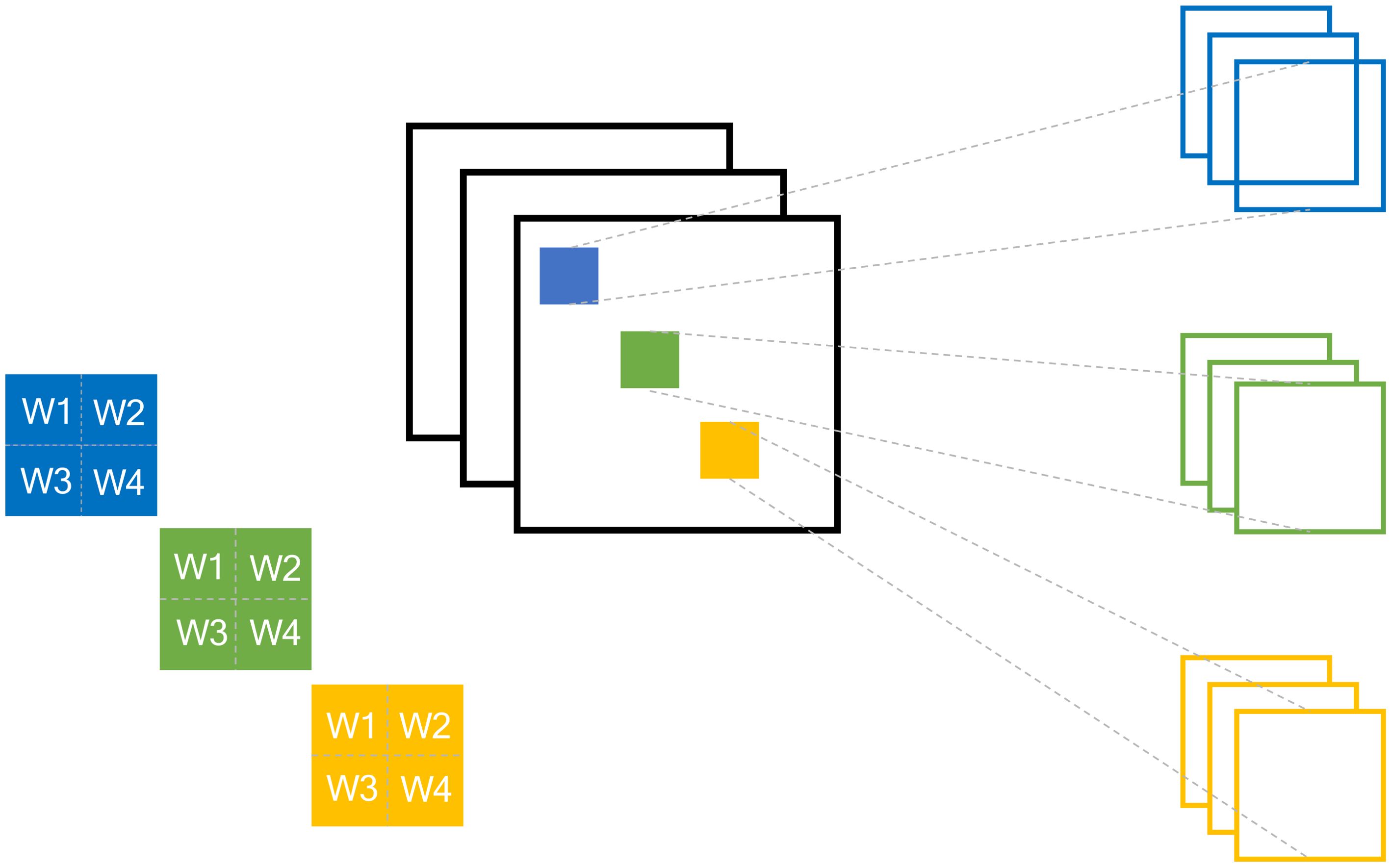
Figure 2. Schematic diagram of the multi-convolutional kernel.

Convolutional neural networks usually contain three types of layers, namely convolutional, pooling and fully connected layers. The convolutional layer performs the input and the convolutional operation of convolutional kernel to extract the features of the input image. The input data of the layer $\text{I}$ is denoted by ${\text{a}}^{\text{I}-1}$ and the output data of the layer $\text{I}$ is denoted by ${\text{a}}^{\text{I}}$, where $\text{I}\in \{1,\dots ,\text{L}\}$. (Equation 1) gives the convolutional layer formula.

$\begin{array}{ll}{\text{a}}_{\text{j}}^{\text{I}}=\text{f}(\sum _{\text{k}}{\text{a}}_{\text{k}}^{\text{I}-1}{\text{*w}}_{\text{jk}}^{\text{I}}+{\text{b}}_{\text{j}}^{\text{I}})& (1)\end{array}$

In the formula:

${\text{w}}_{\text{jk}}^{\text{I}}$ is the convolutional kernel of the kth feature map in layer $\text{I}-1$ to the jth feature map in layer $\text{I}$.

${\text{b}}_{\text{j}}^{\text{I}}$ is the bias of the jth feature map in the layer $\text{ l}$.

$\text{f}(·)$ is the activation function in convolution operation.

The input of the pooling layer is usually the output of the convolutional layer featured with invariance and dimensionality reduction. Feature invariance means that the pooling layer will retain the most dominant features of the image, including rotation, translation and scale invariance. Dimensionality reduction refers to removing some redundant information and decreasing parameters while retaining the key features. In addition to lowering the dimensionality of data characteristics, the pooling layer also aids in reducing the network overfitting, which in turn improves the generalization ability of the model. (Equation 2) gives the formula for pooling layer.

$\begin{array}{ll}{\text{a}}_{\text{j}}^{\text{I}}=\text{downsample}({\text{a}}_{\text{k}}^{\text{I}-1},\text{m})+{\text{b}}_{\text{j}}^{\text{I}}& (2)\end{array}$

In the formula:

${\text{a}}_{\text{k}}^{\text{I}-1}$ is the input data from the kth feature map of layer $\text{I}-1$

${\text{b}}_{\text{j}}^{\text{I}}$ is the bias of the jth feature map in the layer $\text{l}$

$\text{downsample}(·,\text{m})$ is the poling method with the convolutional kernel of $\text{mxm}$

The fully connected layer integrates the characteristic and reduces the impact of feature position. It is the same as a normal neural network that each neuron is connected to every other neuron in the previous layer. In practice, fully connected layers can be implemented by convolutional operations, specifically, a convolutional layer with a convolutional kernel of $1\text{x}1$ can be used to substitute the fully connected layer where the front layer is also fully connected.

The process of convolutional neural network training (Figure 3): the pre-processed sea surface temperature data are first input into the constructed network, and the data are then propagated from the input to the output layer by layer to obtain the prediction result. Next, the predicted output is compared with the input to get the error. Finally, the error of each layer is backward inferenced in the process of back-propagation, and the weights of the convolutional kernel in the corresponding layer is continuously updated.

Figure 3

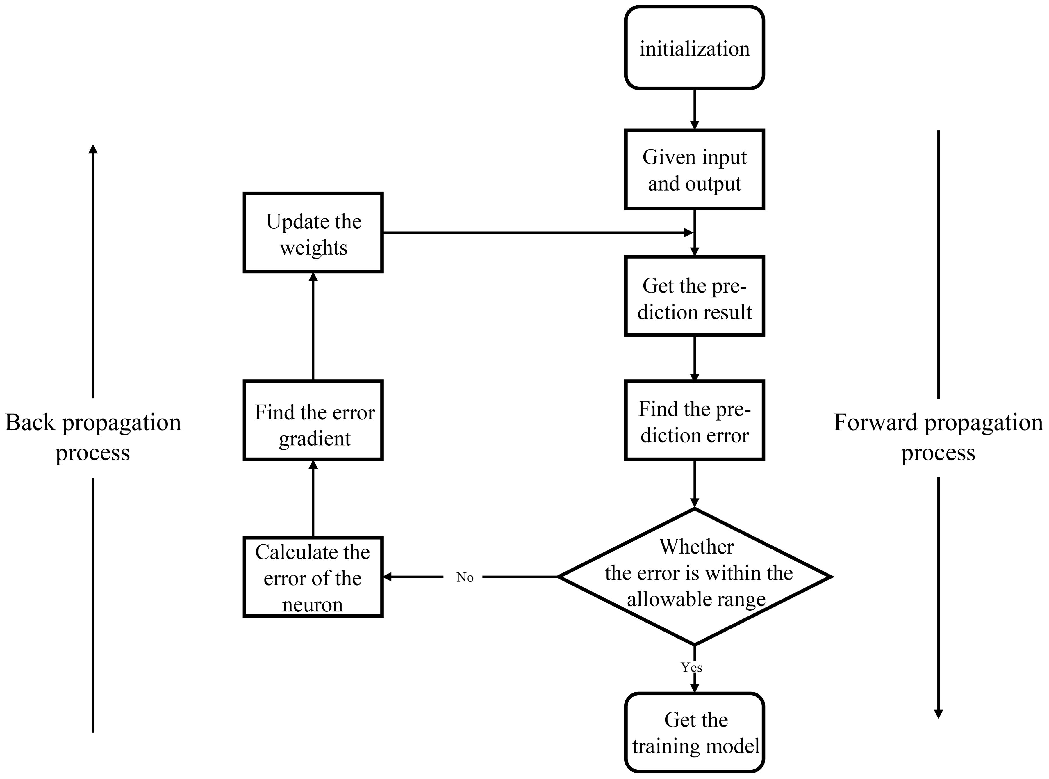
Figure 3. Processing flow of the CNN.

The cost function is obtained by comparing the actual output of the network with the desired output. Assumed that the cost function selected is the mean square error function as shown in (Equation 3).

$\begin{array}{ll}\mathit{C}=\frac{\mathbf{1}}{\mathbf{2}}\sum {({\mathit{y}}^{\mathit{L}}-{\mathit{a}}^{\mathit{L}})}^{\mathbf{2}}& (3)\end{array}$

In this formula, ${\text{a}}^{\text{L}}$ refers to the activation value of the layer L (the output of the activation function) and ${\text{y}}^{\text{L}}$ denotes the desired output of the layer L.

The majority of the convolutional neural network back propagation error is composed of the output layer error and the hidden layer error. The error equation of the output layer is shown in (Equation 4).

$\begin{array}{ll}{\mathit{\delta }}^{\mathit{L}}=\frac{\partial \mathit{C}}{\partial {\mathit{z}}^{\mathit{L}}}=\frac{\partial \mathit{C}}{\partial {\mathit{a}}^{\mathit{L}}}\frac{\partial {\mathit{a}}^{\mathit{L}}}{\partial {\mathit{z}}^{\mathit{L}}}=\frac{\partial \mathit{C}}{\partial {\mathit{a}}^{\mathit{L}}}{\mathit{f}}^{\prime }({\mathit{z}}^{\mathit{L}})=({\mathit{a}}^{\mathit{L}}-{\mathit{y}}^{\mathit{L}}){\mathit{f}}^{\prime }({\mathit{z}}^{\mathit{L}})& (4)\end{array}$

In this formula, ${\text{z}}^{\text{L}}={\text{w}}^{\text{I}}{\text{*a}}^{\text{I}-1}+{\text{b}}^{\text{I}}$ denotes the weight input of each layer and $\text{f}\prime ({\text{z}}^{\text{L}})$ means the derivative of the activation function.

The transfer equation of the error is shown in (Equation 5).

$\begin{array}{ll}{\mathit{\delta }}^{\mathit{I}}=({({\mathit{w}}^{\mathit{I}+\mathbf{1}})}^{\mathit{T}}{\mathit{\delta }}^{\mathit{I}+\mathbf{1}})\mathit{\sigma }({\mathit{z}}^{\mathit{I}})& (5)\end{array}$

This equation shows that we can calculate the error $\text{I}$ of layer $\text{I}$ from the error $\text{I}+1$ in layer $\text{I}+1$. Combining (Equations 4, 5), the error can be calculated of any layer in the network by first calculating $\text{I}$, then $\text{I}-1$, $\text{I}-2,\dots$ till the input layer.

The error in the hidden layer includes the error in the known pooling or convolutional layer. The error of the previous hidden layer can be obtained by back derivation.

As the error of the pooling layer is known, then the error of the previous hidden layer can be deduced backwards.

$\begin{array}{ll}{\mathit{\delta }}^{\mathit{I}-\mathbf{1}}=\mathit{u}\mathit{p}\mathit{s}\mathit{a}\mathit{m}\mathit{p}\mathit{l}\mathit{e}({\mathit{\delta }}^{\mathit{I}}){\mathit{f}}^{\prime }({\mathit{z}}^{\mathit{I}-\mathbf{1}})& (6)\end{array}$

In this formula (Equation 6), $\text{upsample}(·)$ is the upsampling function for the product of Hadamard, which is used for point-to-point multiplication between matrices.

Since the error of the convolutional layer is known, the error of the previous hidden layer can be deduced backwards.

$\begin{array}{ll}{\mathit{\delta }}^{\mathit{I}-\mathbf{1}}={(\frac{\partial {\mathit{z}}^{\mathit{I}}}{\partial {\mathit{z}}^{\mathit{I}-\mathbf{1}}})}^{\mathit{T}}{\mathit{\delta }}^{\mathit{I}}={\mathit{\delta }}^{\mathit{I}}*\mathit{r}\mathit{o}\mathit{t}\mathbf{180}({\mathit{w}}^{\mathit{I}}){\mathit{f}}^{\prime }({\mathit{z}}^{\mathit{I}-\mathbf{1}})& (7)\end{array}$

In this formula (Equation 7), $\text{rot}180({\text{w}}^{\text{I}})$ indicates that the convolutional kernel of layer $\text{l}$ is rotated by 180 degrees and then convolved with the error in layer $\text{l}$. $*$ means the convolutional operation.

$\begin{array}{ll}\frac{\partial \mathit{J}(\mathit{w},\mathit{b})}{\partial {\mathit{w}}^{\mathit{I}}}={\mathit{a}}^{\mathit{I}-\mathbf{1}}*{\mathit{\delta }}^{\mathit{I}}& (8)\end{array}$

Knowing the error of the convolutional layer is shown in (Equation 8), the gradient of w, b in that layer can be derived. $\text{l}$ is the high-dimensional tensor while b is just a vector, so it usually sums the terms of each submatrix of $\text{l}$ separately to obtain an error vector, which is the gradient of b, as shown in (Equation 9).

$\begin{array}{ll}\frac{\partial \mathit{J}(\mathit{w},\mathit{b})}{\partial {\mathit{b}}^{\mathit{I}}}=\sum _{\mathit{u},\mathit{v}}{({\mathit{\delta }}^{\mathit{I}})}_{\mathit{u},\mathit{v}}& (9)\end{array}$

Meanwhile, three indicators, mean absolute error (MAE), (Equation 10), root mean square error (RMSE), (Equation 11) and mean absolute percentage error (MAPE), (Equation 12), were selected for the validation analysis of the prediction results. The three indicators were defined as follows.

$\begin{array}{ll}\mathit{M}\mathit{A}\mathit{E}=\frac{{\sum }_{\mathit{i}=\mathbf{1}}^{\mathit{n}}|{\mathit{y}}_{\mathit{r}\mathit{e}\mathit{a}\mathit{l}}-{\mathit{y}}_{\mathit{p}\mathit{r}\mathit{e}\mathit{d}}|}{\mathit{n}}& (10)\end{array}$

$\begin{array}{ll}\mathit{R}\mathit{M}\mathit{S}\mathit{E}=\sqrt{\frac{{\sum }_{\mathit{i}=\mathbf{1}}^{\mathit{n}}{({\mathit{y}}_{\mathit{r}\mathit{e}\mathit{a}\mathit{l}}-{\mathit{y}}_{\mathit{p}\mathit{r}\mathit{e}\mathit{d}})}^{\mathbf{2}}}{\mathit{n}}}& (11)\end{array}$

$\begin{array}{ll}\mathit{M}\mathit{A}\mathit{P}\mathit{E}=\frac{\mathbf{100}\%}{\mathit{n}}{\displaystyle \sum {}_{\mathit{i}=\mathbf{1}}^{\mathit{n}}}\left|\frac{{\mathit{y}}_{\mathit{r}\mathit{e}\mathit{a}\mathit{l}}-{\mathit{y}}_{\mathit{p}\mathit{r}\mathit{e}\mathit{d}}}{{\mathit{y}}_{\mathit{r}\mathit{e}\mathit{a}\mathit{l}}}\right|& (12)\end{array}$

In these formulae, ${\text{y}}_{\text{real}}$ ata; ${\text{y}}_{\text{pred}}$ is the predicted value of SST data; n is the number of predicted points in the predicted sea area.

3 Temporal and spatial variability characteristics of SST in the NIO

3.1 Spatial distribution of SST in the NIO

The NIO serves as a vital conduit connecting the Pacific and Atlantic shipping routes, and its SST significantly influences global climate. Figure 4 illustrates the spatial distribution of annual mean SST in the NIO from 1980 to 2021. The annual mean SST during this period ranged from 25°C to 30°C. With the exception of the northwestern Arabian Sea, the majority of the NIO exhibited SSTs exceeding 28°C. The distribution of SST shows marked spatial variability, with higher values predominantly located in the central and eastern waters of 0-5°N, where temperatures range from approximately 29°C to 29.5°C; and the Red Sea region can reach temperatures as high as 30°C. In contrast, lower SST values are primarily found in the Persian Gulf and the western boundary of the Arabian Sea, varying between 25°C and 27.5°C. Overall, the annual mean SST displays a trend of increasing values from the northwest to the southeast.

Figure 4

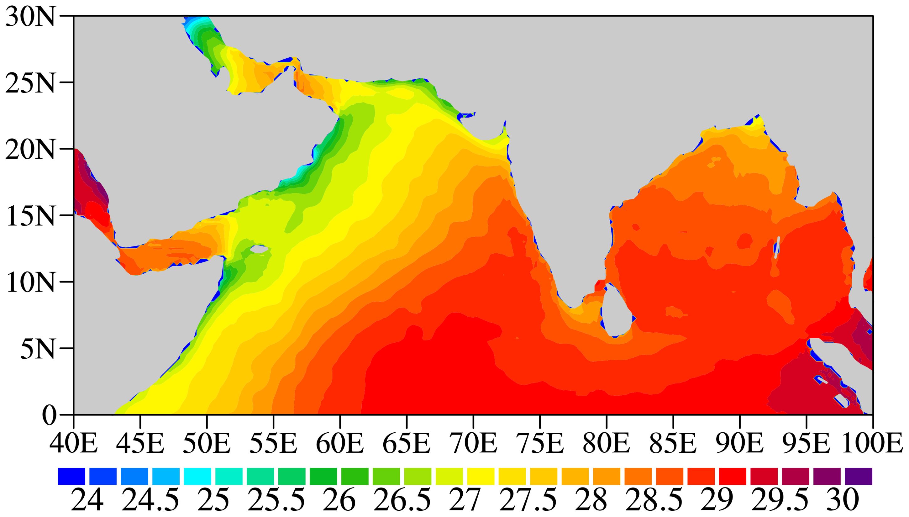
Figure 4. Spatial distribution of annual mean SST (°C) in the NIO from 1980 to 2021.

Figure 5 depicts the seasonal mean SST spatial distribution across four seasons: winter (DJF, December-January-February), spring (MAM, March-April-May), summer (JJA, June-July-August), and autumn (SON, September-October-November). SST values are generally low during winter, with the Persian Gulf averaging 24°C, and the northern and northwestern regions of the Arabian Sea and the northern Bay of Bengal exhibiting temperatures below 26.5°C. In the other regions of the NIO, temperatures range from 27.5°C to 29°C. SST in the NIO reaches its peak in spring, with the spatial distribution characteristics resembling those of winter, but with significantly higher values. The mean temperature in the Persian Gulf remains below 25°C, while the northern Bay of Bengal and the northern and northwestern Arabian Sea range from approximately 26.5°C to 29°C; the mean SST in the central and southern waters of the NIO exceeds 29.5°C. Following the onset of the southwest monsoon, summer SST experiences a decline, with the mean temperature in the western boundary region of the Arabian Sea around 26°C, and most areas of the central and eastern NIO ranging from 28°C to 29°C, not exceeding 29.5°C. In contrast to winter and spring, the mean SST in summer significantly increases to 30°C in the Red Sea and the Persian Gulf. The spatial distribution characteristics of autumn mean SST are similar to those of summer, with the highest temperatures occurring in the Red Sea and the Persian Gulf, reaching up to 30°C. Followed by the central and eastern regions of the NIO, which vary between 27.5°C and 29°C. The lowest values are observed in the western boundary region of the Arabian Sea, ranging from approximately 26.5°C to 27°C.

Figure 5

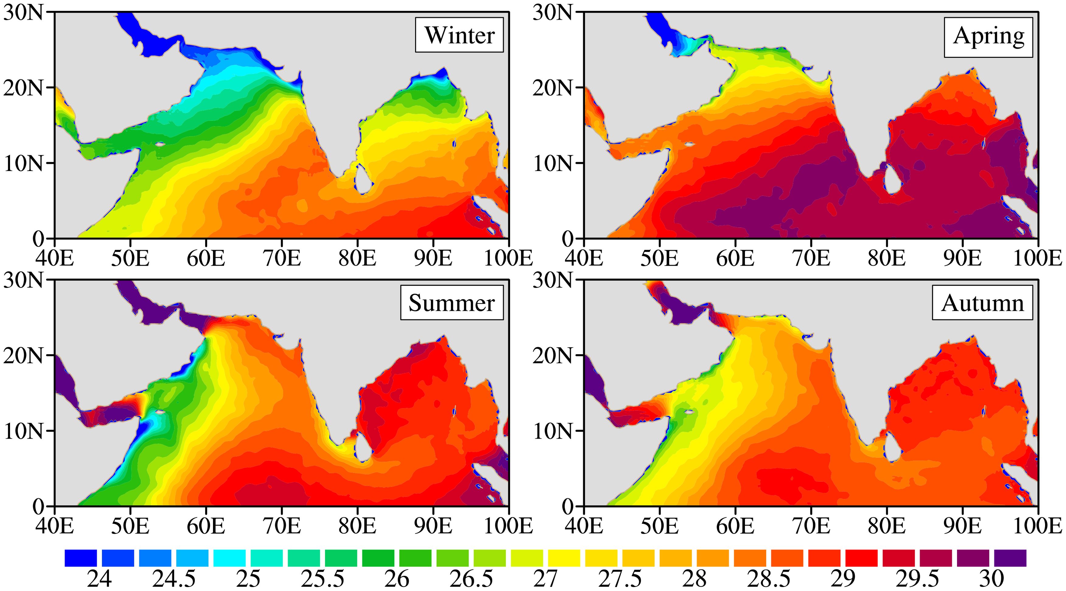
Figure 5. Spatial distribution of seasonal mean SST (°C) in the NIO from 1980 to 2021.

3.2 Low frequency variation and long-term trend of SST in the NIO

Figure 6 illustrates the variations in SST averaged in the NIO from 1980 to 2021. During this period, the annual mean SST exhibited a general upward trend in the NIO. Notably, the highest SST was recorded in 1998, reaching 28.6°C, while the lowest SST occurred in 1984, at only 27.7°C. Overall, the SST in the NIO increased gradually over the 42-year period, with a total rise of approximately 0.5°C (Figure 6).

Figure 6

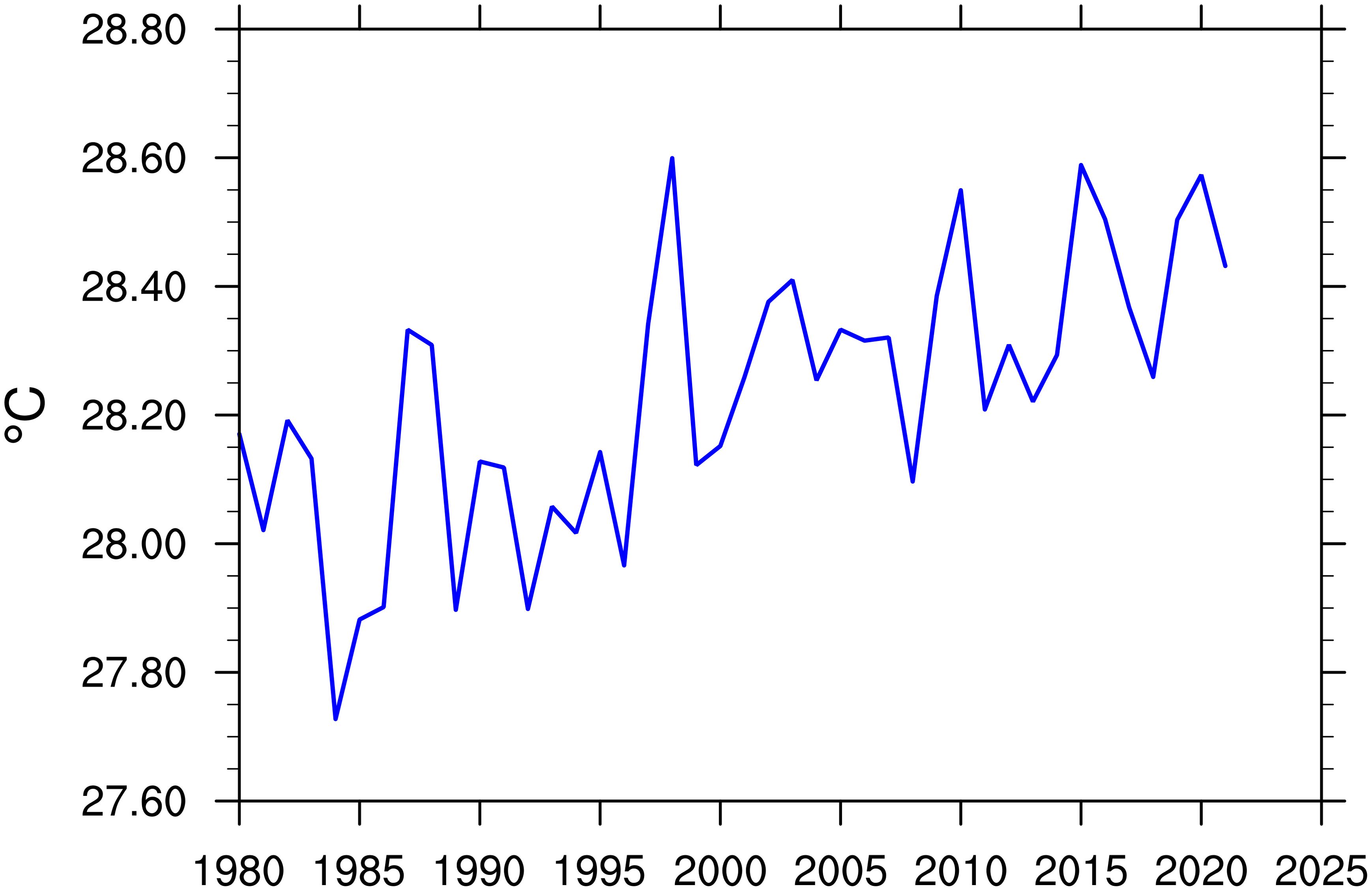
Figure 6. Temporal variability of annual mean SST (°C) in the NIO from 1980 to 2021.

The seasonal variations in SST in the NIO from 1980 to 2021 are illustrated in Figure 7. Numerically, the SST is highest in spring, followed by summer and autumn, with winter exhibiting the lowest values. An analysis of trends reveals a gradual increase in the mean SST across all four seasons over the study period. The warming trends in summer, autumn, and winter are relatively consistent, while the warming trend in spring is more moderate. The figure also indicate that the seasonal SST in the NIO reached its peak in 1998, 2010 and 2016 (Figure 7).

Figure 7

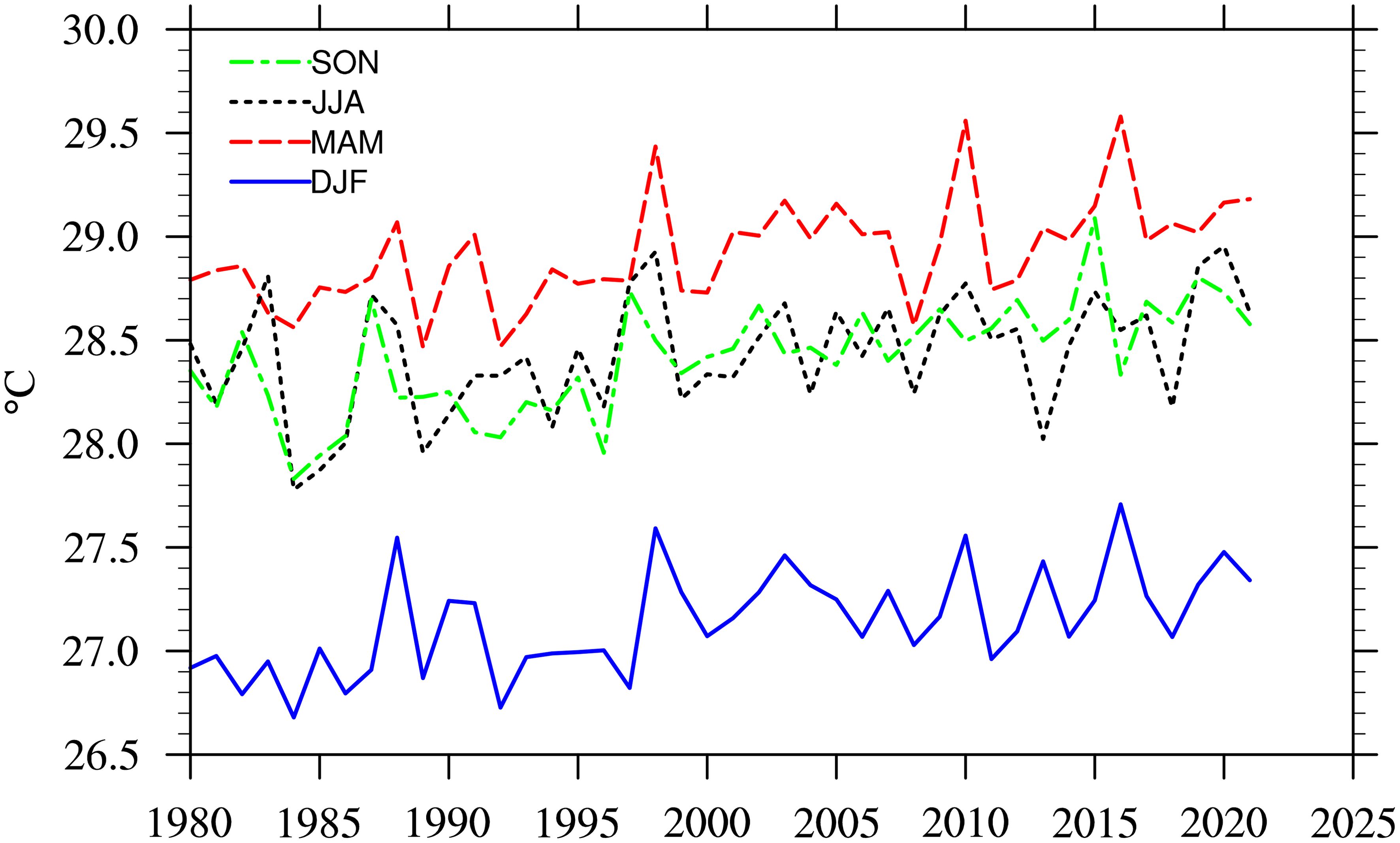
Figure 7. Temporal variability of seasonal mean SST (°C) in the NIO from 1980 to 2021.

3.3 EOF analysis of SST in the NIO

The variations in SST exhibit distinct spatial distribution characteristics in the NIO. The application of EOF method allows for the decomposition of related eigenvectors, which better reflects the spatial distribution structure and temporal variability of SST changes. The variance contribution rates of the first three eigenvalues derived from the EOF analysis are 28.4%, 10.1%, and 7.7% respectively, with a cumulative contribution rate of 46.2%. Significance testing indicates that the EOF analysis results are reasonable and effectively explain the primary distribution characteristics of SST in the NIO from 1980 to 2021. Given the negligible variance contribution rates of subsequent modes, which do not significantly influence the overall spatial modal distribution, this study will concentrate on the first three modes to derive more meaningful research outcomes results. The first EOF mode (EOF-1) explains 28.4% of the total variance, and exhibits a basin-wide uniform warming pattern over the Indian Ocean (Figure 8a), corresponding to the Indian Ocean Basin Mode (IOBM) (Yang et al., 2007; Du et al., 2009). The first principal component (PC-1) shows a maximum positive correlation (r = 0.67) with the Nino3.4 index at a 3-4-month lag, which aligns with the typical occurrence of IOBM in boreal spring following an El Niño event. Furthermore, this basin-scale warming plays a crucial role in maintaining the anomalous anticyclonic circulation over the western North Pacific during post-El Niño years (Xie et al., 2009; Wu et al., 2010).

Figure 8

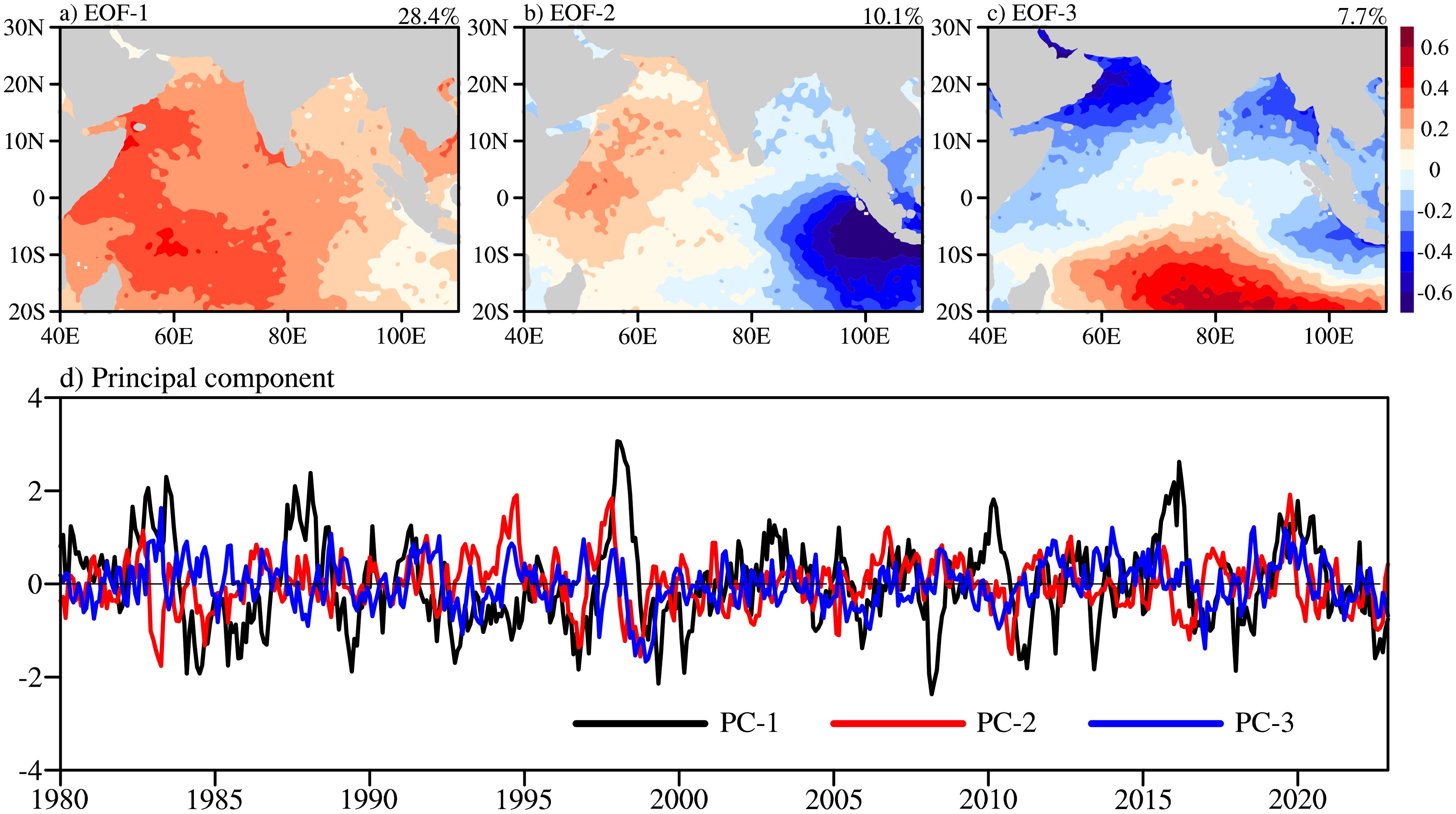
Figure 8. The first three EOF modes and the associated principal components of the SST in the NIO.

The second EOF mode (EOF-2), accounting for 10.1% of the variance, displays the characteristic zonal dipole pattern of the Indian Ocean Dipole (IOD) (Saji et al., 1999; Webster et al., 1999). This mode features pronounced cold SST anomalies in the eastern Indian Ocean, particularly along the Java-Sumatra coast, accompanied by relatively weak warming in the western basin (Figure 8b). The IOD typically peaks in autumn, with the second principal component (PC-2) showing maximum positive correlation when leading the Nino3.4 index by 3-4 months.

The third EOF mode (EOF-3) explains 7.7% of the variance, and manifests as a tripole pattern, characterized by warming in the south-central tropical Indian Ocean flanked by cooling anomalies in both the western and southeastern Indian Ocean. This SST distribution has been termed the Indian Ocean Tripole (IOT) (Zhang et al., 2020; Chen et al., 2024b), Southern Tropical Indian Ocean Dipole (STIOD) (Zhang et al., 2024), or IOD Modoki (Endo and Tozuka, 2016; Tozuka et al., 2016). This mode has emerged since the mid-1970s (Du et al., 2013), its occurrence is linked to the Australian Monsoon variation (Chen et al., 2024b), and could affect the surface air temperature over the western Tibetan Plateau in summer (Zhu et al., 2024).

3.4 Results of correlation analysis between SST and different meteorological factors

Studies indicate that the SST significantly influences the global climate, and the distribution of substances and momentum in the ocean by wind, heating, cooling, precipitation, and evaporation (Wang, 2003). Although the SST variations are relatively small in magnitude, integrated changes can also significantly affect local precipitation, atmospheric circulation, and the monsoon (Hu et al., 2005; Zhang et al., 2015). In this paper, considered the influence of several hydro-meteorological factors on the SST, we analyzed the correlation between them in a multidimensional way, selecting six meteorological data, including 10m zonal wind, 10m meridional wind, 2m dew-point temperature, 2m air temperature, mean sea level pressure, and total cloud cover, conducted correlation analysis between each element and the SST in the north Indian Ocean (Figure 9). The results show the SST has a high positive correlation with 2m dew-point temperature and 2m air temperature under the interaction of heat transfer between sea and air (Figures 9a, b); the correlation between meridional and zonal wind speed and the SST reveals significant spatial differences (Figures 9c, d). Without considering other factors such as dynamics, the higher temperature, the faster the atmospheric heat expansion rises and the lower the air pressure, thus, the SST shows a good negative correlation with MSLP, especially in the northern part of the Bay of Bengal and the Arabian Sea (Figure 9e). As the total cloud cover can enhance the backward radiation of the atmosphere to the surface and plays the role of insulation, it shows a positive correlation distribution with the SST, but the influence is relatively small compared with other meteorological factors (Figure 9f).

Figure 9

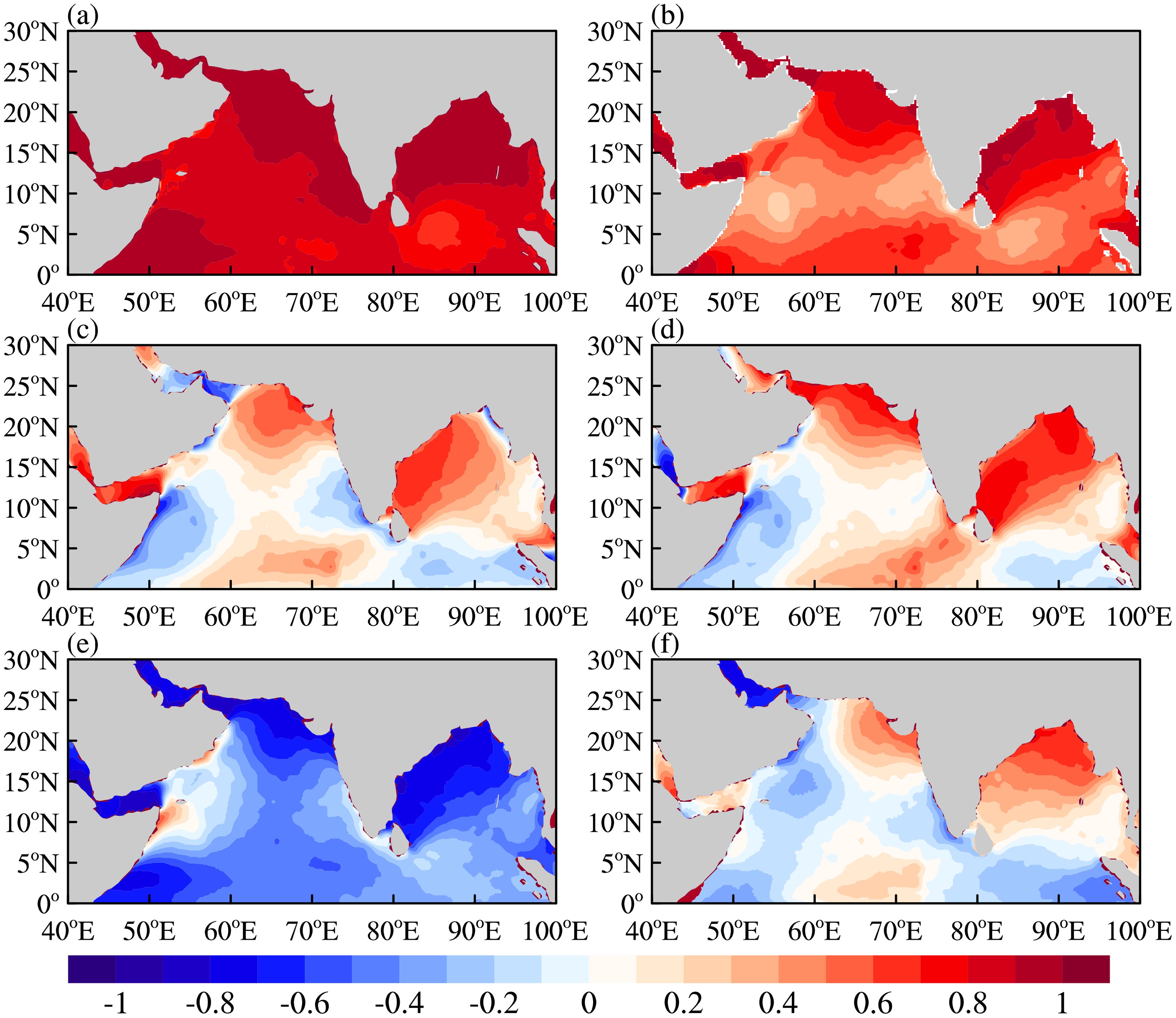
Figure 9. Correlation coefficients between T2M and SST (a), D2M and SST (b), U10 and SST (c), V10 and SST (d), MSLP and SST (e), and TCC and SST (f) in the NIO from 1980 to 2020.

4 Construction of deep learning model based on SST prediction

4.1 Construction of SST prediction model

The effects of the six meteorological elements mentioned above on the SST vary from different regions due to influenced by dynamic oceanography and topographic environment. Thus, in order to build a more accurate SST prediction model for the NIO, in this paper, the matrix composed of six day-by-day meteorological elements for the next seven days and SST data of the previous day from 2001 to 2020 is used as the input term of the prediction model. As for output term, a matrix of SST data for the following seven days is used as well. After training large number of prediction model point by point for the whole NIO, a SST forecast model for the next week can be built based on the current data (Figure 10).

Figure 10

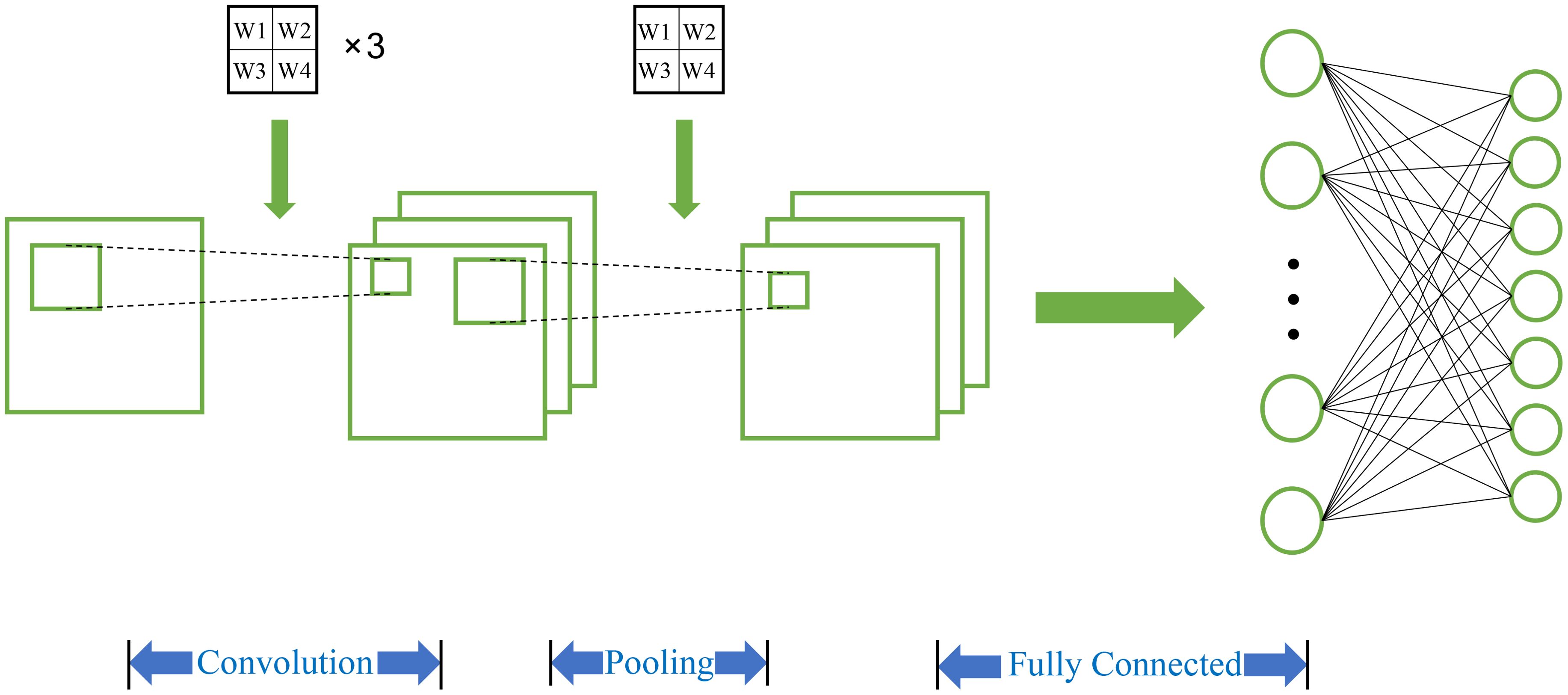
Figure 10. Schematic diagram of SST forecast model structure.

According to Figure 10, the input data is convoluted to produce the feature map of the second layer, after downsampling, it is pooled to create the third layer feature map. So as to get the SST data for the next seven days, the feature map is finally linked into vectors by row expansion and sent into the fully connected layer. Meanwhile, in order to increase the nonlinearity of the neural network model, an activation function is added in order to introduce the nonlinear factors to the neurons, so that the neural network can freely approximate any nonlinear function. The biggest issue with deep learning is the gradient disappearance, which is especially problematic in the case of using saturated activation functions such as tanh and sigmoid (when the neural network is propagating directional errors, each layer is multiplied by the first order derivative of the activation function, and the gradient decays with each passing layer. The gradient G keeps decaying until it disappears when there are more layers in the network), which makes the training network converge more and more slowly. Therefore, this paper uses the linear, non-saturated form of the Relu function as the activation function, which has the following functional form.

$\begin{array}{ll}\mathit{f}(\mathit{x})=\mathit{m}\mathit{a}\mathit{x} (\mathbf{0},\mathit{x})& (13)\end{array}$

This function overcomes the problem of gradient disappearance and accelerate training. The results of sea surface temperature prediction for the next seven days can be obtained ultimately.

4.2 Forecast results and analysis

To ensure that there is no overlap or dependency between the training data and the test data, the data set used in this study is divided into three categories: the data from 2001 to 2020 as the training set, the data from 2021 as the validation set, and the data from January 2022 as the test set. After the training is completed, which is carried out by using the training data, the model results are obtained. In order to avoid underfitting or overfitting, the model must be evaluated by using the validation data. Test data can be used for prediction after finding the best parameters. At the same time, using the sample generator for training can better solve the problem of traditional forecast models that cannot be trained due Massive data in training. Using the forecast model constructed in this paper, the SST for the 2nd week of 2022 can be respectively predicted.

From the prediction results (Figure 11), it can be concluded that the day-by-day prediction results of SST in the NIO are basically consistent with the measured results. The sea regions with large SST prediction errors change with the number of prediction days (Figure 11c), and the errors get larger as the number of predicted days rise. Except for some regions, the absolute value of the SST prediction error in the NIO is basically stable within 1°C, and it does not exceed 0.5°C in most of the regions (Figure 11c). The graphs of SST prediction results (Figures 11a, b) preserve the contour information and distribution characteristics of the actual images as a whole, and are the same as the real variation pattern of the NIO in terms of spatial and temporal variation patterns.

Figure 11

Figure 11. Results of measured data (a), predicted results (b) and prediction errors (°C) (c) for the 2nd week of 2022.

From the error analysis of the SST prediction results in the NIO using three error assessment criteria (Figure 12), it can be observed that the overall prediction errors in the NIO increase as the number of prediction days rise and it presents an upward tendency. Besides, the smooth increase in the three errors indicates that the forecast model has strong stability.

Figure 12

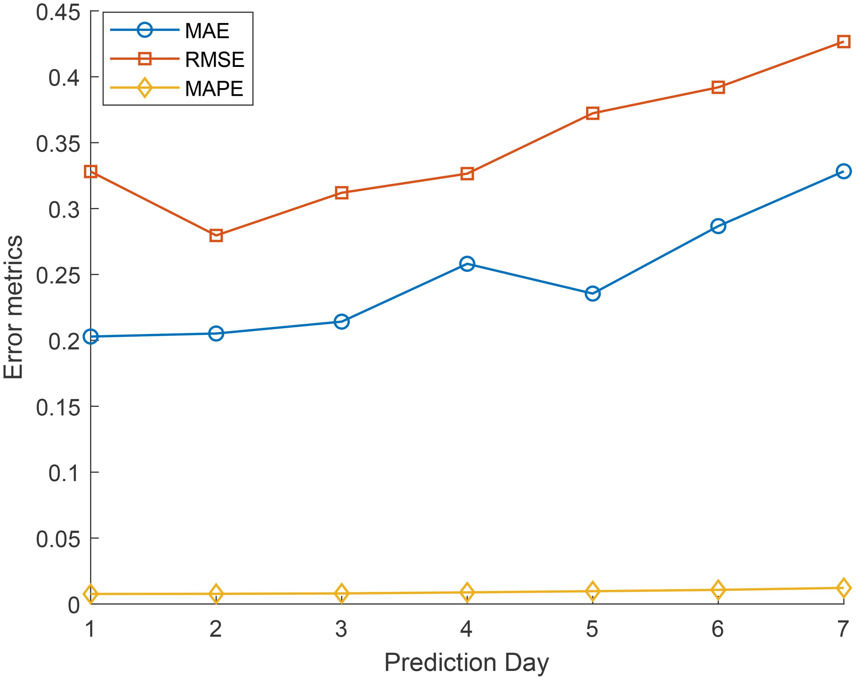
Figure 12. Error statistics of predicted the SST data in the NIO (°C).

5 Discussion and conclusion

5.1 Discussion

In this paper, the SST predication model based on CNN deep learning constructed is an attempt to predict the SST in the NIO. The advantage of this model over previous SST forecast models is that it overcomes the traditional thinking of single method prediction and combines the numerical model of the ocean with the data-driven model in a clever way. Besides, it takes the professional marine theoretical knowledge as the basis and uses the marine meteorological element in space and time to strengthen the regional distribution information of natural position and improve its regional and overall applicability effect. However, the model also has shortcomings. Firstly, the multivariate model in this paper is constrained by the amount of data as deep learning has a high requirements of data. The influence factors used in the forecast model need to be further analyzed for the intrinsic influence with the SST. Appropriate additions and deletions need to be made to improve the learning and prediction capacity of the SST forecast model. Secondly, there is still room for further optimization of the CNN network built in this paper to get improved prediction outcomes. In summary, it is feasible to use the CNN model to predict the sea surface temperature, and the prediction accuracy is relatively high in the study regions. It offers a fresh perspective on the prediction of sea surface temperature in the NIO.

5.2 Conclusion

SST is a crucial component of the marine environment, serving as a pivotal variable for understanding the interactions between the ocean and the atmosphere. It plays a significant role in shaping climate and marine environments. In this study, we employed ERA5 data and EOF to analyze the spatiotemporal variations of SST in the NIO. The results show that the SST in the NIO increases year by year from 1980 to 2021, with the highest value in spring, followed by summer and autumn, and the lowest value in winter. EOF analysis of SST shows that the cumulative contribution rate of the first three modes reaches 46.2%, EOF-1 explaining 28.4% of the total variance, exhibits a basin-wide uniform warming pattern over the Indian Ocean. EOF-2 accounts for 10.1% of the variance and exhibits the IOD pattern. EOF-3 explaining 7.7% of the variance, displays a tripole distribution characterized by warming in the central tropical southern Indian Ocean and cooling in the western and southeastern Indian Ocean. This SST distribution pattern is referred to as the IOT, STIOD, or IOD Modoki.

The study further investigated the relationships and impacts of various meteorological factors on SST, analysis of these six meteorological variables revealed that air-sea heat exchange and topographical conditions significantly influence the SST in the NIO. based on these findings, a CNN-based SST prediction model was developed. The prediction results indicated that the model maintained a prediction error generally within 1°C, with errors in most regions of the NIO not exceeding 0.5°C. The predicted results preserved the contour information and distribution characteristics of the actual SST, aligning with the temporal and spatial variation patterns observed in the NIO. Evaluation of the prediction results using error assessment standards showed that as the prediction period increased, the SST prediction error exhibited an overall upward trend, with a stable rate of increase, indicating the robustness of the proposed prediction model.

Data availability statement

The original contributions presented in the study are included in the article/supplementary material. Further inquiries can be directed to the corresponding author.

Author contributions

WH: Formal Analysis, Writing – original draft. HL: Data curation, Methodology, Writing – review & editing. TZ: Writing – review & editing. ZC: Resources, Supervision, Writing – review & editing.

Funding

The author(s) declare that financial support was received for the research and/or publication of this article. This study was supported by Research on Major Issues of Entrusting Agent Ownership of Natural Resource Assets and Asset Inventory Project of Guangdong Province (440000220000000002496); Pilot Project of the Inventory of Natural Resources Assets Owned by the Whole People in Guangdong Province (440000210000000001073); Survey and Evaluation of Typical Ecosystems in Key Coastal Areas of Guangdong Province (440000220000000007742); and Monitoring and Evaluation of Marine Ecological Restoration Engineering Based on UAV Remote Sensing (440000240000000002901).

Acknowledgments

The ERA5 data is maintained and provided by European Centre for Medium-Range Weather Forecasts (ECMWF). We acknowledge the reviewers.

Conflict of interest

Author ZC was employed by the company CCC-FHDI Engineering Co., Ltd.

The remaining authors declare that the research was conducted in the absence of any commercial or financial relationships that could be construed as a potential conflict of interest.

Generative AI statement

The author(s) declare that no Generative AI was used in the creation of this manuscript.

Publisher’s note

All claims expressed in this article are solely those of the authors and do not necessarily represent those of their affiliated organizations, or those of the publisher, the editors and the reviewers. Any product that may be evaluated in this article, or claim that may be made by its manufacturer, is not guaranteed or endorsed by the publisher.

References

Aparna S. G., D’souza S., Arjun N. B. (2018). Prediction of daily sea surface temperature using artificial neural networks. Int. J. Remote Sens. 39, 4214–4231. doi: 10.1080/01431161.2018.1454623

Crossref Full Text | Google Scholar

Ashok K., Guan Z., Yamagata T. (2003). Influence of the Indian Ocean Dipole on the Australian winter rainfall. Geophys. Res. Lett. 30(15). doi: 10.1029/2003GL017926

Crossref Full Text | Google Scholar

Chakravorty S., Chowdary J. S., Gnanaseelan C. (2013). Epochal changes in the seasonal evolution of tropical Indian Ocean warming associated with El Niño. Clim. Dyn. 42,, 1–18. doi: 10.1007/s00382-013-1666-3

Crossref Full Text | Google Scholar

Chen L. T., Jin Z. Y., Luo S. H. (1985). Characteristics of SST changes in the Indian Ocean and the South China Sea and some links with atmospheric circulation. J. Oceanogr. 1, 103-110.

Google Scholar

Chen M., Collins M., Yu J. Y., Wang X., Zhang L., Tam C. Y. (2024b). Emerging influence of the Australian Monsoon on Indian Ocean interannual variability in a warming climate. Clim. Atmos. Sci. 7, 319. doi: 10.1038/s41612-024-00879-9

Crossref Full Text | Google Scholar

Chen Q., Cai C., Chen Y., Zhou X., Zhang D., Peng Y. (2024a). TemproNet: A transformer-based deep learning model for seawater temperature prediction. Ocean Eng. 293, 116651. doi: 10.1016/j.oceaneng.2023.116651

Crossref Full Text | Google Scholar

Dong Z. J., Teng J., Wang Y. P. (2008). Application of phase space reconstruction and ANFIS modelin SST forecasting. J. Trop. Oceanogr. 27, 73–76. doi: 10.3969/j.issn.1009-5470.2008.04.011

Crossref Full Text | Google Scholar

Donguy J. R., Meyers G. (1996). Seasonal variations of sea-surface salinity and temperature in the tropical Indian Ocean. Deep-Sea Res. Part I. 43, 117–138. doi: 10.1016/0967-0637(96)00009-x

Crossref Full Text | Google Scholar

Du Y., Cai W., Wu Y. (2013). A new type of the Indian Ocean Dipole since the mid-1970s. J. Clim. 26, 959–972. doi: 10.1175/JCLI-D-12-00047.1

Crossref Full Text | Google Scholar

Du Y., Xie S. P., Huang G., Hu K. (2009). Role of air–sea interaction in the long persistence of El Niño–induced north Indian Ocean warming. J. Clim. 22, 2023–2038. doi: 10.1175/2008JCLI2590.1

Crossref Full Text | Google Scholar

Endo S., Tozuka T. (2016). Two flavors of the Indian Ocean dipole. Clim. Dyn. 46, 3371–3385. doi: 10.1007/s00382-015-2773-0

Crossref Full Text | Google Scholar

Fang K., Yu J. H. (2019). Influence of sea surface temperature gradients in the tropical Pacific and Indian oceans of the Northern Hemisphere on the frequency of tropical cyclone generation in the western North Pacific in summer. J. Trop. Oceanogr. 38, 42–51. doi: 10.11978/2018136

Crossref Full Text | Google Scholar

Fu Y., Song J., Guo J., Fu Y., Cai Y. (2024). Prediction and analysis of sea surface temperature based on LSTM-transformer model. Reg. Stud. Mar. Sci. 78, 103726. doi: 10.1016/j.rsma.2024.103726

Crossref Full Text | Google Scholar

Garcia-Gorriz E., Garcia-Sanchez J. (2007). Prediction of sea surface temperatures in the western Mediterranean Sea by neural networks using satellite observations. Geophys. Res. Lett. 34(11). doi: 10.1029/2007GL029888

Crossref Full Text | Google Scholar

Hamza F. R., Priotti J. P. (2020). Maritime trade and piracy in the Gulf of Aden and the Indian Ocean, (1994–2017). J. Transp. Secur. 13, 141–158. doi: 10.1007/s12198-018-0190-4

Crossref Full Text | Google Scholar

He Q., Zha C., Song W., Hao Z., Du Y., Liotta A., et al. (2020). Improved particle swarm optimization for sea surface temperature prediction. Energies. 13, 1369. doi: 10.3390/en13061369

Crossref Full Text | Google Scholar

Hu R. J., Liu J. Y., Meng X. F., Godfrey J. S. (2005). On the mechanism of the seasonal variability of SST in the tropical Indian Ocean. Adv. Atmos. Sci. 22, 451–462. doi: 10.1007/BF02918758

Crossref Full Text | Google Scholar

Izumo T., Montégut C. B., Luo J. J., Behera S. K., Masson S., Yamagata T. (2008). The role of the western Arabian Sea upwelling in Indian monsoon rainfall variability. J. Clim. 21, 5603–5623. doi: 10.1175/2008JCLI2158.1

Crossref Full Text | Google Scholar

Ji J. X., Zhang L. F. (2010). Prediction of sea surface temperature by Kalman filtering. Mar. Fore 27, 59–65.

Google Scholar

Jiang Y., Gou Y., Zhang T., Wang K., Hu C. (2017). A machine learning approach to argo data analysis in a thermocline. Sensors. 17, 2225. doi: 10.3390/s17102225

PubMed Abstract | Crossref Full Text | Google Scholar

Khan M. Z. K., Sharma A., Mehrotra R. (2018). Using all data to improve seasonal sea surface temperature predictions: A combination-based model forecast with unequal observation lengths. Int. J. Climatol. 38, 3215–3223. doi: 10.1002/joc.5494

Crossref Full Text | Google Scholar

Krizhevsky A., Sutskever I., Hinton G. E. (2017). ImageNet classification with deep convolutional neural networks. Commun. ACM. 60, 84–90. doi: 10.1145/3065386

Crossref Full Text | Google Scholar

Noori R., Abbasi M. R., Adamowski J. F., Dehghani M. (2017). A simple mathematical model to predict sea surface temperature over the northwest Indian Ocean. Estuar. Coast. Shelf Sci. 197, 236–243. doi: 10.1016/j.ecss.2017.08.022

Crossref Full Text | Google Scholar

Saji N. H., Goswami B. N., Vinayachandran P. N., Yamagata T. (1999). A dipole mode in the tropical Indian Ocean. Nature. 401, 360–363. doi: 10.1038/43854

PubMed Abstract | Crossref Full Text | Google Scholar

Stockdale T. N., Balmaseda M. A., Vidard A. (2006). Tropical Atlantic SST prediction with coupled ocean–atmosphere GCMs. J. Clim. 19, 6047–6061. doi: 10.1175/JCLI3947.1

Crossref Full Text | Google Scholar

Tao W., Huang G., Hu K., Qu X., Wen G., Gong Y. (2013). Different influences of two types of El Niños on the Indian Ocean SST variations. Theor. Appl. Climatol 117, 475–484. doi: 10.1007/s00704-013-1022-x

Crossref Full Text | Google Scholar

Tozuka T., Endo S., Yamagata T. (2016). Anomalous Walker circulations associated with two flavors of the Indian Ocean Dipole. Geophys. Res. Lett. 43, 5378–5384. doi: 10.1002/2016GL068639

Crossref Full Text | Google Scholar

Wang Q. (2003). A research on the short-term numerical prediction of the sea surface temperature over the East China Sea. J. Ocean China 3, 32–43.

Google Scholar

Webster P. J., Moore A. M., Loschnigg J. P., Leben R. R. (1999). Coupled ocean–atmosphere dynamics in the Indian Ocean during 1997–98. Nature. 401, 356–360. doi: 10.1038/43848

PubMed Abstract | Crossref Full Text | Google Scholar

Wu A., Hsieh W. W., Tang B. (2006). Neural network forecasts of the tropical Pacific sea surface temperatures. Neural Netw. 19, 145–154. doi: 10.1016/j.neunet.2006.01.004

PubMed Abstract | Crossref Full Text | Google Scholar

Wu B., Li T., Zhou T. (2010). Relative contributions of the Indian Ocean and local SST anomalies to the maintenance of the western North Pacific anomalous anticyclone during the El Niño decaying summer. J. Clim. 23, 2974–2986. doi: 10.1175/2010JCLI3300.1

Crossref Full Text | Google Scholar

Xiao C., Chen N., Hu C., Wang K., Xu Z., Cai Y., et al. (2019). A spatiotemporal deep learning model for sea surface temperature field prediction using time-series satellite data. Environ. Model. Software 120, 104502. doi: 10.1016/j.envsoft.2019.104502

Crossref Full Text | Google Scholar

Xie S. P., Hu K., Hafner J., Tokinaga H., Du Y., Huang G., et al. (2009). Indian Ocean capacitor effect on Indo–western Pacific climate during the summer following El Niño. J. Clim. 22, 730–747. doi: 10.1175/2008JCLI2544.1

Crossref Full Text | Google Scholar

Xu L., Li Y., Yu J., Li Q., Shi S. (2020). Prediction of sea surface temperature using a multiscale deep combination neural network. Remote Sens. Lett. 11, 611–619. doi: 10.1080/2150704X.2020.1746853

Crossref Full Text | Google Scholar

Yang M., Ding Y., Li W., Mao H. Q., Huang C. (2008). The leading mode of Indian Ocean SST and its impacts on Asian summer monsoon. Acta Meteor. Sinica. 22, 31.

Google Scholar

Yang J., Liu Q., Xie S. P., Liu Z., Wu L. (2007). Impact of the Indian Ocean SST basin mode on the Asian summer monsoon. Geophys. Res. Lett. 34(4). doi: 10.1029/2006GL028571

Crossref Full Text | Google Scholar

Yang L. Q., Wang L. N., Zhang H. C., Dong C. M. (2024). Combining forecasting model for sea surface temperature in the South China Sea based on STL. Mar. Environ. Sci. 43, 109–118. doi: 10.12111/j.mes.2023-x-0167

Crossref Full Text | Google Scholar

Zhang Y., Li J., Zhao S., Zheng F., Feng J., Li Y., et al. (2020). Indian Ocean tripole mode and its associated atmospheric and oceanic processes. Clim. Dyn. 55, 1367–1383. doi: 10.1007/s00382-020-05331-1

Crossref Full Text | Google Scholar

Zhang Q., Wang H., Dong J., Zhong G., Sun X. (2017). Prediction of sea surface temperature using long short-term memory. IEEE Geosci. Remote Sens. Lett. 14, 1745–1749. doi: 10.1109/LGRS.2017.2733548

Crossref Full Text | Google Scholar

Zhang G., Wang X., Xie Q., Huang B., Chen J., Fan H., et al. (2024). Attributing interdecadal variations of southern tropical Indian Ocean dipole mode to rhythms of Bjerknes feedback intensity. Clim. Dyn. 62, 3841–3857. doi: 10.1007/s00382-024-07102-8

Crossref Full Text | Google Scholar

Zhang X. D., Zhang W. L., Li Y. B. (2015). Characteristics of the sea temperature in the North Yellow Sea. Mar. Fore. 32, 89–97. doi: 10.11737/j.issn.1003-0239.2015.05.011

Crossref Full Text | Google Scholar

Zhou L., Yang C. Y., Wang H. J., Zhao S. X. (2009). Interpretation scheme of SST predjction in the tropical Pacific Ocean based on CCA-BP-BPNN. J. PLA Univ. Sci. Technol. 4, 391–396. doi: 10.7666/j.issn.1009-3443.20090417

Crossref Full Text | Google Scholar

Zhou T. J., Yu R. C., Li W., Zhang X. H. (2001). On the variability of the Indian Ocean during the 20th century. Acta Meteorol. Sin. 59, 257–270. doi: 10.11676/qxxb2001.028

Crossref Full Text | Google Scholar

Zhu M., Zhang Y., Li J., Liu T., Hou Z., Wang H. (2024). Physical connection between the tropical Indian Ocean tripole and western Tibetan Plateau surface air temperature during boreal summer. Clim. Dyn. 62, 9703–9718. doi: 10.1007/s00382-024-07418-5

Crossref Full Text | Google Scholar