Preprocessing LOFARgram through U-Net++ neural network

The study of the low-frequency analysis and recording spectrum (LOFARgram) of ship-radiated noise is essential for extracting critical information, such as target motion trajectories. However, the quality of LOFARgrams often degrades due to the inherent stochasticity of ship noise and the interference of environmental noise. We significantly enhance the clarity and quality of LOFARgrams by employing the U-Net++ neural network model for preprocessing. Effective training of neural network models usually requires large datasets, but the available actual LOFARgrams are often limited and costly to collect. To ensure an adequate dataset for neural network training, this paper introduces an innovative forward model that simulates LOFARgrams from stochastic noise sources. This model uses explosive decaying cosine pulses as basic units to simulate ship noise sources and employs the KRAKEN normal mode model to simulate the underwater acoustic channel’s transfer function, thereby efficiently creating high-fidelity ship noise LOFARgrams. The forward model supplies sufficient data to train the U-Net++ neural network, enabling it to demonstrate effective recovery of LOFARgrams. Additionally, we introduce a new algorithm that utilizes data prior to the Closest Point of Approach (CPA) to predict the CPA parameters, applied to both the original LOFARgrams and those processed with U-Net++. Results indicate that predictions based on U-Net++ enhanced LOFARgrams are more accurate. Our work demonstrate the effectiveness of the forward model and U-Net++ enhanced LOFARgrams for ship-radiated noise analysis and precise prediction of target motion.

1 Introduction

During the propagation of sound waves in shallow sea areas, interference phenomena occur among various normal modes. When the received signal from the target sound source is converted to the time-frequency domain, a stable and observable interference structure with geometric distribution is formed, typically represented by a LOFARgram. Numerous scholars have conducted theoretical and experimental studies on sound field interference structures. S.D. Chuprov proposed the theory of waveguide invariant β (Chuprov and Brekhovskikh, 1982), highlighting the relationship between the slope of the interference structure and the waveguide invariant. D. Rouseff extracted the slopes of interference fringes in LOFARgrams using different methods (Rouseff and Leigh, 2002). Song et al. used the adiabatic approximation to explain the reasons for the different slopes of interference fringes before and after CPA of a target in a sloping seabed scenario (Song et al., 2022). LOFARgrams have been widely studied and applied due to its significant source information. T. C. Yang indicated that the interference structure of the sound field also has good applications in anti-interference (Yang, 2003). Target motion parameters can be estimated based on sound field interference structures (Li et al., 2016). The presence of a target can be determined and tracked by observing line spectra in LOFARgrams (Chen et al., 2021). And differences in the structure of LOFARgrams can be used to distinguish between incoming and outgoing ships (Guo et al., 2023).

Despite the significant value of LOFARgrams in research and application, the quality of the collected data is often poor, as shown in Figure 1A. The signals received by hydrophones are subject to interference from environmental noise, leading to discontinuities in the LOFARgrams. And the slowly time-varying characteristics of the oceanic channel can affect both the amplitude and phase of the signals. Additionally, factors such as low source levels of target radiated noise and variations in radiated noise intensity can cause the interference fringes in LOFARgrams to become blurred, resulting in a low signal-to-noise ratio (SNR) and making them difficult to utilize effectively. To overcome these issues and further improve the performance of LOFARgrams, preprocessing is generally required. Common signal processing methods include Principal Component Analysis (PCA), Empirical Mode Decomposition (EMD), 2-Dimensional Fast Fourier Transform (2DFFT), and low-pass filtering. These methods may prove effective in preprocessing LOFARgrams.

Figure 1

Figure 1. Simulation of LOFARgrams. (A) The measured LOFARgram of the Qingdao Sea Area. (B) Time-frequency diagram of waveguide transfer function. (C) Time-frequency diagram of the received signal. (D) Time-frequency diagram of the received signal with Added Gaussian White Noise, the SNR is set at −20dB.

Many studies employ deep learning methods to address underwater acoustics challenges, such as detecting, identifying, and classifying underwater targets using deep learning networks (Chen et al., 2021). Additionally, research has utilized convolutional neural networks to recover latent line spectrum structures in LOFARgrams from background interference (Han et al., 2020). The recovery effect far surpasses the perceptual range of human vision in traditional line spectrum detection, enabling the detection and recovery of line spectra with lower signal-to-noise ratios. This paper aims to use U-Net++ neural network to preprocess LOFARgrams.

Neural network models require sufficient training data to ensure their reliability and stability. However, due to the discrete distribution of actual ship-radiated noise, collecting LOFARgrams is both costly and time-consuming. Therefore, relying solely on measured data is often insufficient for training the neural network model. To address the issue of insufficient data, this paper proposes a forward model for simulating LOFARgrams of stochastic acoustic sources. This forward model is composed of the ship noise source model and the underwater acoustic channel model, with the Gaussian white noise. For the sound source model, this paper combines the physical process of ship-generated radiated noise sources and uses an exponentially decaying cosine pulse as the basic unit. The time-domain signals of radiated noise from different parts of the ship are represented as a superposition of a series of pulse sequences. By adjusting the pulse shape, timing, duration, intensity, and period, the difference between the simulated power spectrum and the measured ship noise power spectrum can be minimized, achieving a simulation of the ship-radiated noise. This method is well-suited for simulating mechanical noise and propeller noise of ships (Jun-Ping et al., 2016). For the channel model, the KRAKEN normal mode acoustic field model is employed to simulate the underwater channel transfer function. Finally, Gaussian white noise is added to the two models to simulate ship noise LOFARgrams, enabling efficient dataset construction.

We choose the U-Net++ neural network for the preprocessing of LOFARgrams. U-Net++ is a architecture based on nested and dense skip connections (Zhou et al., 2018), capable of effectively capturing features at different scales and efficiently separating noise from true image characteristics. This architecture aids in detail preservation during image restoration tasks, resulting in clear images and reduced boundary blur. Furthermore, U-Net++ can be flexibly adjusted for various image restoration tasks, demonstrating strong generalization capabilities. In this paper, we constructed a dataset using a forward model and trained the U-Net++ model. By fitting the training data, U-Net++ can significantly enhance the quality of the LOFARgrams, achieving excellent restoration results.

This study employs the Closest Point of Approach (CPA) parameter estimation algorithm to analyze the effectiveness of U-Net++ in restoring LOFARgrams. The interference fringes in the LOFARgrams contain information about the target’s closest point of approach, with the lowest point of the fringes corresponding to the target’s time of closest approach. By applying the CPA parameter estimation algorithm to the LOFARgrams prior to the CPA point, it is possible to predict information such as the target’s closest approach time. The results indicate that the LOFARgrams processed by U-Net++ exhibit more accurate predictions compared to the unprocessed versions, demonstrating the superior performance of U-Net++ in the recovery of LOFARgrams.

The structure of this paper is as follows: Section 2 introduces the fundamental theory of LOFARgrams. Section 3 elaborates on the forward model for simulating ship LOFARgrams, which serves as the basis for constructing the dataset for the neural network. Section 4 demonstrates the preprocessing effectiveness of the U-Net++ neural network on LOFARgrams, achieving satisfactory recovery results. Section 5 evaluates the preprocessing performance of U-Net++ on LOFARgrams by applying the CPA parameter estimation algorithm to both the original and preprocessed LOFARgrams. This algorithm utilizes the LOFARgram to predict target motion parameters before reaching the CPA, revealing that U-Net++ preprocessing enhances the predictive accuracy of the estimation algorithm. Section 6 summarizes the conclusions.

2 Basic theory of LOFARgram

Russian scientist S.D. Chuprov first introduced the concept of the waveguide invariant β while studying the interference structure of the acoustic field in ocean waveguides within the space-frequency r − ω domain. The expression of the waveguide invariant is as follows

$\begin{array}{ll}\beta =\frac{r}{\omega }\frac{\partial \omega }{\partial r},& (1)\end{array}$

where ω is the signal frequency, r is the horizontal distance between the sound source and the receiving hydrophone, and ∂ω/∂r is the slope of the internal interference fringes in the (r − ω) domain.

As shown in Figure 2, assume the target is moving in a straight line at a constant speed v. The hydrophone is located at point O. The closest point of approach (CPA) distance relative to the hydrophone is $r_{\mathrm{C}\mathrm{P}\mathrm{A}}$, and the time of the closest point of approach is $t_{\mathrm{C}\mathrm{P}\mathrm{A}}$.

Figure 2

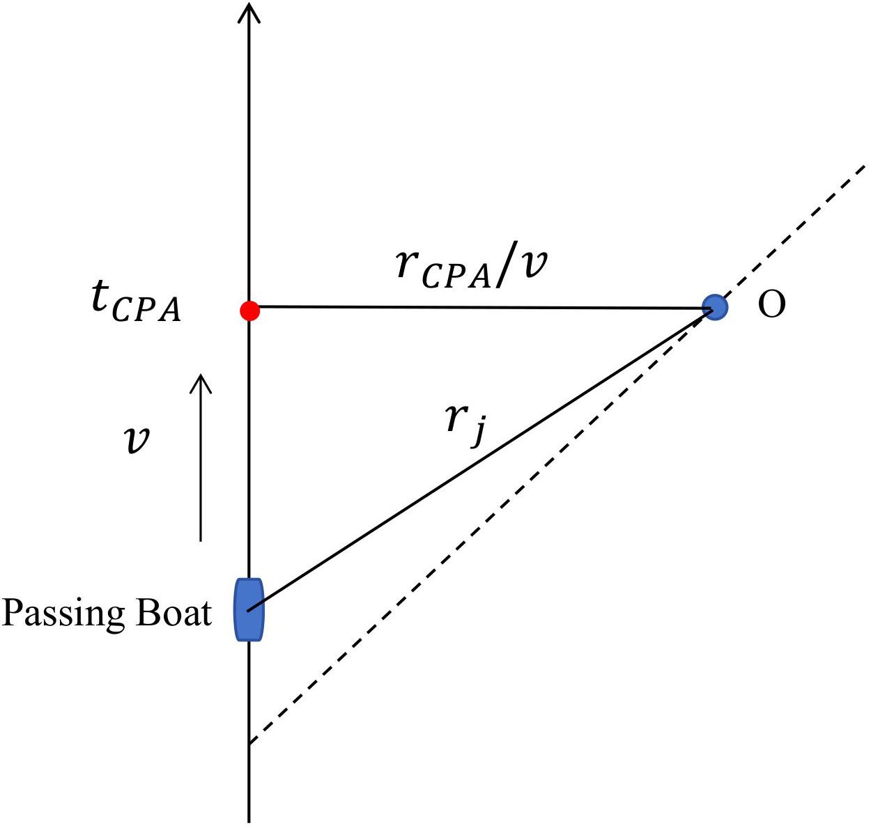
Figure 2. Schematic diagram of target motion geometry.

Based on the geometric relationship shown in the figure, at time t, the distance between the target and the hydrophone O is r(t)

$\begin{array}{ll}r(t)=\sqrt{v^2{(t-t_{\text{CPA}})}^2+r_{\text{CPA}}^2}.& (2)\end{array}$

Differentiate Equation 2

$\begin{array}{ll}\frac{\mathrm{d}\mathrm{r}}{\mathrm{d}\mathrm{t}}=\frac{v^2(t-t_{\mathrm{C}\mathrm{P}\mathrm{A}})}{\sqrt{v^2{(t-t_{\mathrm{C}\mathrm{P}\mathrm{A}})}^2+r_{\mathrm{C}\mathrm{P}\mathrm{A}}^2}}.& (3)\end{array}$

The definition of Equation 1 is in the r − ω domain, but in the LOFARgram, we are more interested in the results in the t − f domain (ω = 2πf). Therefore, we convert the Equation 1 to

$\begin{array}{ll}\beta =\frac{r}{f}\frac{\partial f}{\partial r}.& (4)\end{array}$

The slope of the interference fringes df/dt can be expressed as

$\begin{array}{ll}\frac{df}{dt}=\frac{df}{dr}\frac{dr}{dt}.& (5)\end{array}$

In the t − f domain intensity plot, the slope of the interference fringes is

$\begin{array}{ll}\frac{\text{d}f}{\text{d}t}=\frac{\text{d}f}{\text{d}r}\frac{\text{d}r}{\text{d}t}=\beta \frac{f}{r}{v}_d,& (6)\end{array}$

where $v_d=dr/dt$ is the rate of change of distance between the moving target and the hydrophone, representing the radial velocity of the target relative to the hydrophone.

The Equation 6 can be equivalently written as

$\begin{array}{ll}\frac{\text{d}f}{f}=\frac{\beta v^2(t-t_{\mathrm{C}\mathrm{P}\mathrm{A}})}{v^2{(t-t_{\mathrm{C}\mathrm{P}\mathrm{A}})}^2+r_{\mathrm{C}\mathrm{P}\mathrm{A}}^2}\mathrm{d}\mathrm{t}.& (7)\end{array}$

By integrating both sides of Equation 7 and rearranging, we obtain

$\begin{array}{ll}\text{ln }f=\beta \text{ln }\left(\sqrt{v^2{(t-t_{\text{CPA}})}^2+r_{\text{CPA}}^2}\right)+C_0.& (8)\end{array}$

Given $f_0$ as the vertex frequency of the interference fringes, then $f=f(t)$, $f_0=f(\tau )$, taking the logarithm of the above equation yields

$\begin{array}{ll}f=f_0{\left[1+{\left(\frac{v}{r_{\text{CPA}}}\right)}^2{(t-t_{\text{CPA}})}^2\right]}^{\beta /2}.& (9)\end{array}$

In shallow water, considering the general case β = 1, Equation 9 can be simplified to

$\begin{array}{ll}\frac{f^2}{f_0^2}-\frac{{(t-t_{\mathrm{C}\mathrm{P}\mathrm{A}})}^2}{{(r_{\mathrm{C}\mathrm{P}\mathrm{A}}/v)}^2}=1.& (10)\end{array}$

From Equation 10, it can be understood that the interference pattern when the target passes closest to the hydrophone is a cluster of generalized hyperbolas. Their common parameters are τ and $r_{\mathrm{C}\mathrm{P}\mathrm{A}}/v$.

Equation 10 represents a hyperbolic equation, indicating that the ideal LOFARgram of ship noise should exhibit a clear hyperbolic structure in the interference fringe pattern, as shown in Figure 1B. However, the stochasticity of ship noise and environmental interference can lead to discontinuities and blurriness in the measured LOFARgram, as depicted in Figure 1A. Therefore, simulating the LOFARgram must account for not only the target scenario but also the stochasticity of noise and environmental factors. This paper develops a forward model to simulate the measured LOFARgram, providing a sufficient dataset for the U-Net++ neural network.

3 Forward model for simulated LOFARgram

The formula for the received signal of ship-radiated noise is as follows

$\begin{array}{ll}y(\omega )=s(\omega )h(\omega )+n(\omega ),& (11)\end{array}$

$s(\omega )$ represents the radiated noise signal produced by the ship, consisting of sounds generated by mechanical equipment, engines, propellers, etc. $h(\omega )$ represents the underwater acoustic channel transfer function, indicating the influence of the transmission path from the ship to the receiver. It describes characteristics such as attenuation, propagation delay, and phase changes during underwater sound wave propagation. $n(\omega )$ is Gaussian white noise, with various stochastic noise sources in the underwater environment, such as waves, wind, and underwater creatures, superimposed on the received signal, affecting its clarity and identifiability. The formula for SNR is as follows

$\begin{array}{ll}SNR=20\text{lg }\frac{{\sigma }_1}{{\sigma }_2},& (12)\end{array}$

where ${\sigma }_1$, ${\sigma }_2$ is the variance of $s(\omega )$ $h(\omega )$, $n(\omega )$, respectively.

According to Equation 11, this paper proposes a forward model to simulate the hydrophone received signal $y(\omega )$. Figure 3 shows the specific structure of the forward model, which includes three components: the ship radiated noise model, which simulates the measured ship noise $s(\omega )$; the acoustic field model, which uses the sound propagation calculation model KRAKEN to obtain the channel transfer function $h(\omega )$; and the random noise model, which adds Gaussian white noise to simulate random noise in the ocean environment after superimposing $h(\omega )$ and $s(\omega )$.

Figure 3

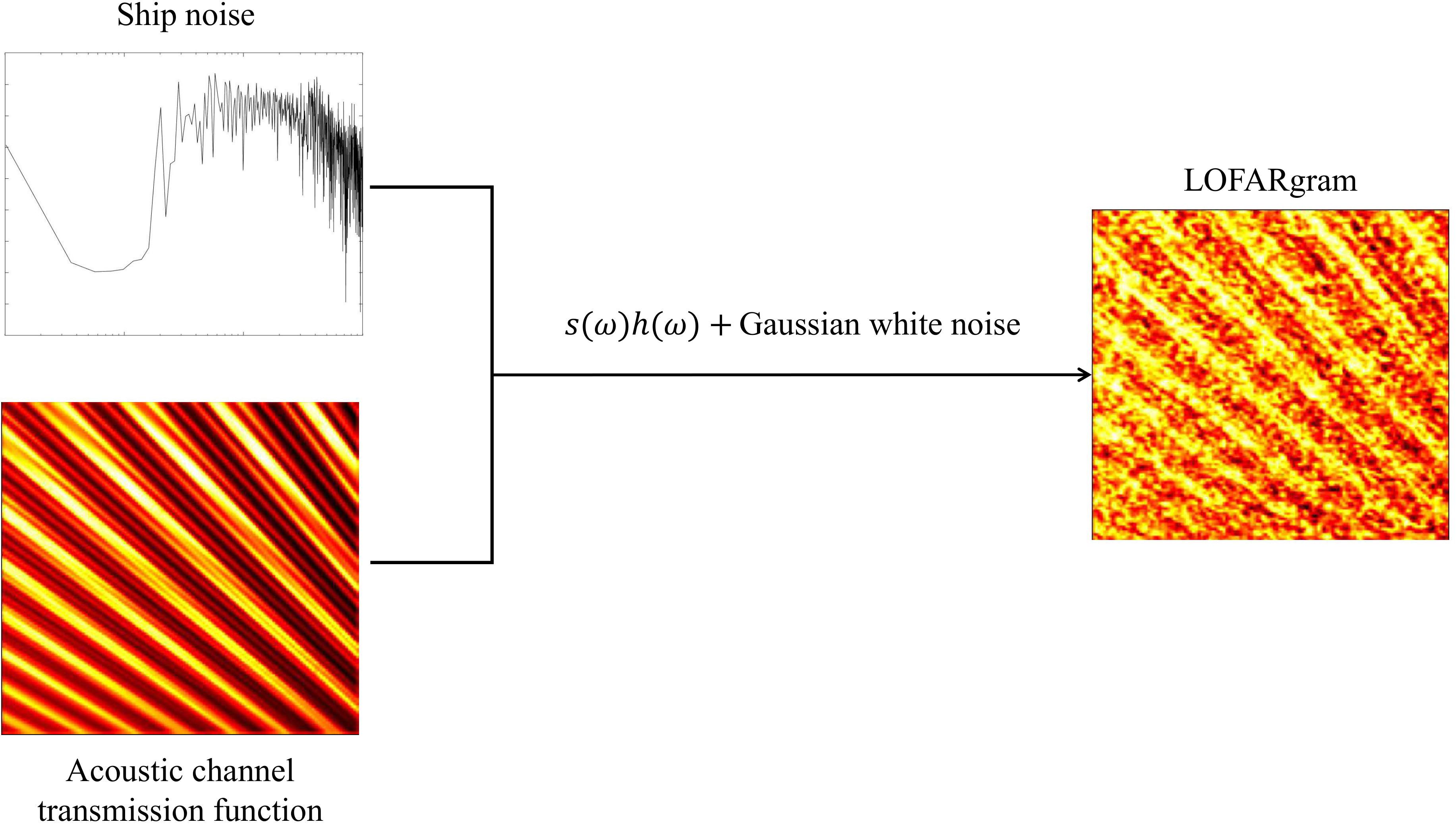
Figure 3. Forward model flow chart.

3.1 Ship noise model

Ships generate both periodic and stochastic noise signals during navigation. Periodic signals typically are generated by the cyclic rotations of mechanical components such as motors, internal combustion engines, and propellers. In contrast, stochastic noise signals arise from ships’ intrinsic characteristics (e.g., speed, depth, tonnage, and propeller parameters). Ship-radiated underwater noise signals can be simulated by various methods (Zhengyao and Yipeng, 2005; Zheng et al., 2020; Zhao et al., 2022). The most common model is traditional sinusoidal wave model (Liu et al., 2019; Guo et al., 2023). This model stimulates periodic noise with superimposed sinusoidal waves and simulates stochastic noise with filtered Gaussian white noise. However, it has notable limitations. The line spectrum obtained by sinusoidal superposition often fail to fully represent the periodic noise characteristics of ship-generated signals. Moreover, stochastic noise signals derived from filtered Gaussian white noise do not sufficiently capture the stochastic variations induced by the marine environment and acoustic channels. Additionally, spectrum with different power require different filters, which limits the practicability and flexibility. Consequently, although the traditional sinusoidal wave model can approximate ship noise to some extent, it falls short in describing complex stochastic processes, particularly instantaneous features and stochastic components.

Considering both the generation process and the stochasticity of ship-radiated noise, this work uses exponentially decaying cosine pulses with a quasi-periodic distribution to simulate ship-radiated noise (Peng et al., 2019; Jun-Ping et al., 2016). The introduction of a quasi-periodic stochastic sequence distribution enhances the representation of the instantaneous characteristics and stochasticity of ship-radiated noise. Moreover, the power spectrum peak of the exponentially decaying cosine pulses can vary with the ship’s speed, enabling more flexible modeling of the dynamic and stochastic changes in the spectral characteristics of ship-radiated noise. In conclusion, the simulation method proposed in this work effectively models the noise induced by both the ship’s mechanical motion and the marine environment, which better capture the variation patterns of ship-radiated noise power spectrum. The formula forhanical motion and the marine environment.

This study adopts exponentially cosine pulses as the basic units of the noise signal, which can be expressed as

$\begin{array}{ll}P=\{\begin{array}{ll}{\text{e}}^{-\text{γ}t}\text{cos }({\omega }_{0}t),\hfill & t\ge 0\hfill \\ -{\text{e}}^{\text{γ}t},\hfill & t<0\hfill \end{array} (\text{γ}>0),& (13)\end{array}$

where γ is the pulse decay coefficient, and ω₀ is the angular frequency.

Furthermore, the pulse sequence is subjected to a quasi-periodic stochastic distribution. Generate N × M explosive decaying cosine pulses, with M pulses superimposed in each column to form N pulse clusters with a period of T. Within a pulse cluster, the generation times of different pulses exhibit a stochastic fluctuation following a Rayleigh distribution. Between different pulse clusters, the standard deviation ${\sigma }_{\mathrm{\Delta }}$ of the stochastic fluctuation follows a normal distribution with a mean of 0. The N pulse clusters are arranged in chronological order to generate a quasi-periodic stochastic pulse sequence of ship-radiated noise signals, and their power spectrum is obtained. At this stage, the simulated power spectrum roughly matches the general shape of the measured ship noise. Finally, by adjusting the pulse cluster period T, the standard deviation ${\sigma }_{\mathrm{\Delta }}$ of the pulse cluster period fluctuation, and the unit pulse amplitude ${\xi }_a$, decay coefficient γ, and cosine frequency ${\omega }_0$, the power spectral characteristics of the ship-radiated noise can be modulated to gradually reduce the differences between the simulated and measured spectra. The specific steps are shown in Figure 4.

Figure 4

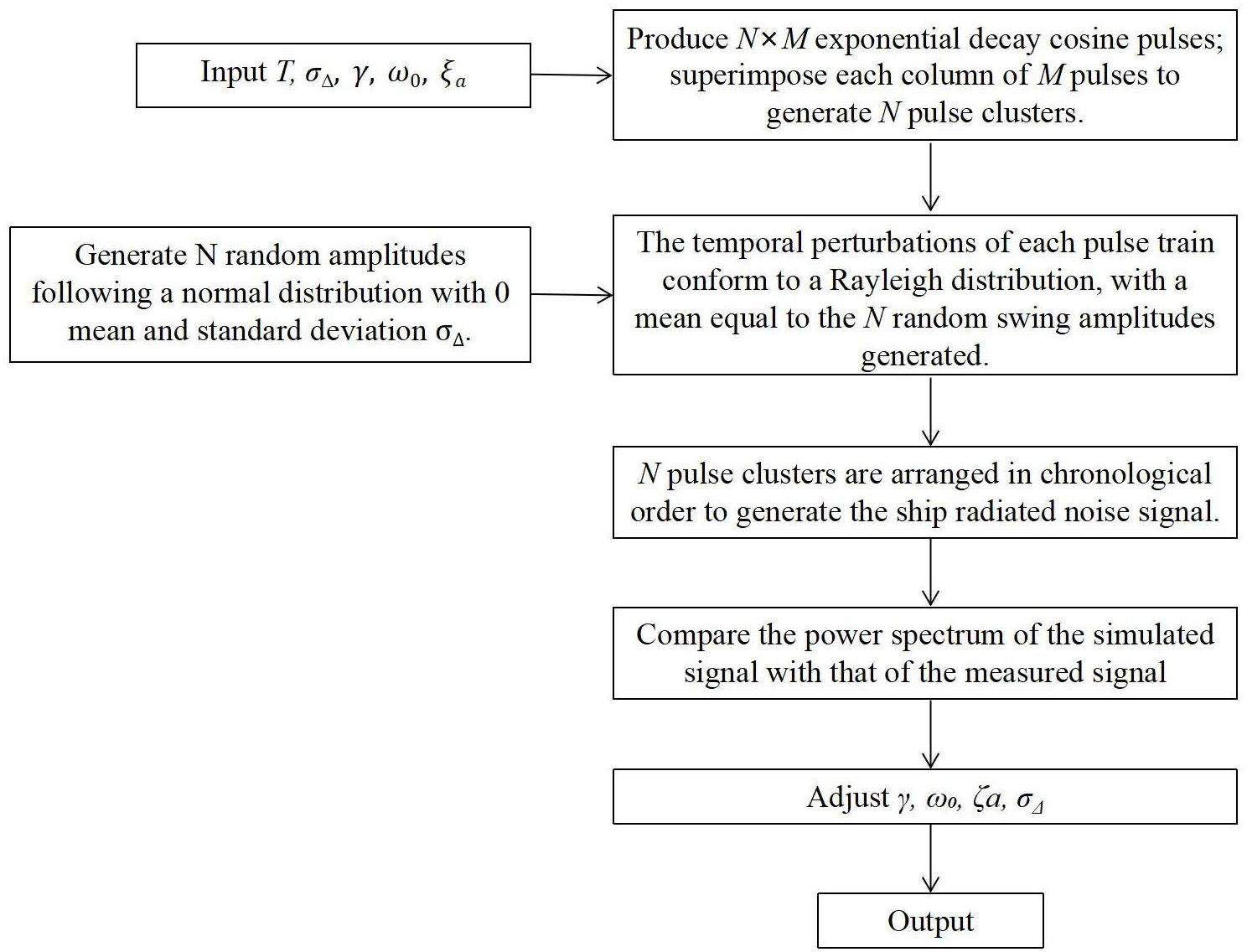
Figure 4. Flow diagram of simulated ship-radiated noise.

We simulated the measured noise of a ship using a quasi-periodic random distribution of explosive cosine pulses. Figure 5 presents a comparison between the measured and simulated ship-radiated noise power spectrum. The blue curve represents the power spectrum of the measured ship noise (Jun-Ping et al., 2016), while the red curve corresponds to the simulated ship-radiated noise power spectrum. It is evident that the simulated power spectrum aligns well with the measured ship-radiated noise characteristics, with a similarity coefficient of 0.85188. This demonstrates that the simulation method employed in this study is both feasible and effective for modeling ship-radiated noise.

Figure 5

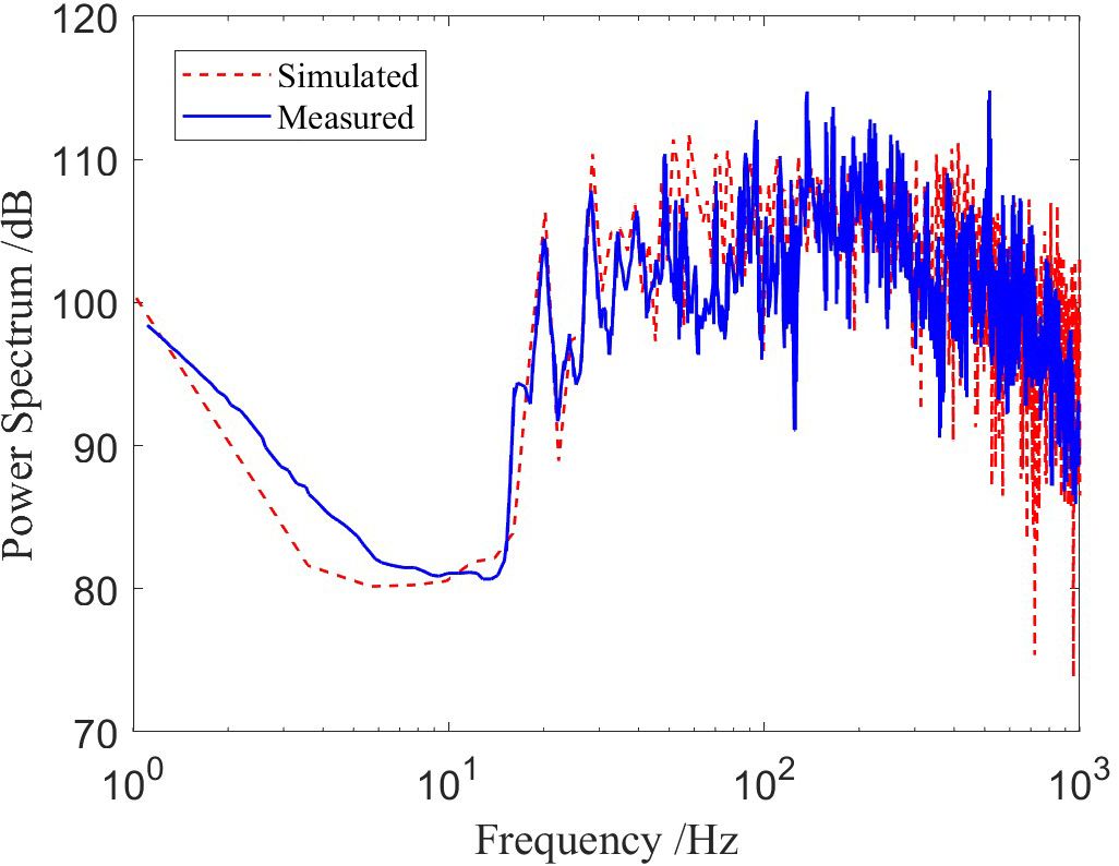
Figure 5. Comparison of measured spectrum and simulated spectrum.

3.2 Transfer function simulation

In this section, the underwater acoustic propagation software KRAKEN (Porter, 1992) is used to simulate the transfer function $h(\omega )$ of the channel.

For low-frequency underwater acoustic channels, the channel transfer function can be given by the normal mode model

$\begin{array}{ll}h(r,\omega )\approx \frac{i}{\rho (z_s)\sqrt{8\pi r}}{\text{e}}^{-\text{j}\pi /4}\sum _{m=1}^{\infty }{\text{Ψ}}_m(z_s){\text{Ψ}}_m(z_r)\frac{{\mathrm{e}}^{j{k}_m(\omega )r}}{\sqrt{k_m(\omega )}},& (14)\end{array}$

where $r$ is the distance between the source and the receiver, $\omega$ is the angular frequency of the sound wave, and $\rho (z_s)$ is the density at the source depth $z_s$, $z_r$ represents the receiver depth, $k_m$ represents the horizontal wavenumber, and ${\text{Ψ}}_m$ represents the eigenfunction.

The main environment and parameters for the simulation are as follows. A surface ship travels at a constant speed v, with a single hydrophone placed underwater to receive broadband signals. The seabed topography is a typical horizontal seabed. The sound speed in the seabed is set to 1550m/s, the seabed density is 1.76 g/cm³, and the seabed attenuation is 0.1 dB/λ. The sound speed profile is chosen to be that of the Yellow Sea region. According to the source model, the unit pulse angular frequency ω₀ of the sound source is $10·2\pi$, and the attenuation coefficient γ = 100. The source depth z_s = 5m; the receiver depth z_r = 20m; t_CPA = 650s; r_CPA = 2000m; and the speed v = 8m/s. The two-dimensional structure diagram is shown in the figure. To calculate the spectrum of the received hydrophone signal and generate a time-frequency diagram in MATLAB, the signal can be divided into segments of 2 seconds each, the spectrum of each segment can be calculated, and all the spectrum data can be concatenated, as shown in Figure 1B. It contains information about the location of the sound source and can be used to estimate the CPA. This noise-free sound transmission image will serve as the learning target and label for the neural network in the following sections. By varying parameters such as z_s, v, and r_CPA, the channel transfer function h(ω) under different conditions can be obtained.

Multiply the ship-radiated noise spectrum by the transfer function spectrum, and concatenate them to obtain the LOFARgram as shown in Figure 1C. Use the randn function to generate the corresponding Gaussian white noise, and finally add the generated noise to the original signal, as shown in Figure 1D.

4 U-Net++ for LOFARgram preprocessing

4.1 Traditional preprocessing methods

Empirical Mode Decomposition (EMD) (Huang et al., 1998) is a traditional signal processing method. EMD is an adaptive signal processing method that decomposes complex signals into a set of intrinsic mode functions. EMD decomposes signals based on the intrinsic time-scale features of the data, without the need for pre-defined basis functions. This allows EMD to be applied theoretically to decompose any types of signal, providing significant advantages in analyzing non-stationary and nonlinear data. We use EMD to preprocess low-quality LOFARgrams, and the results are shown in Figure 6 “EMD Recovered”.

Figure 6

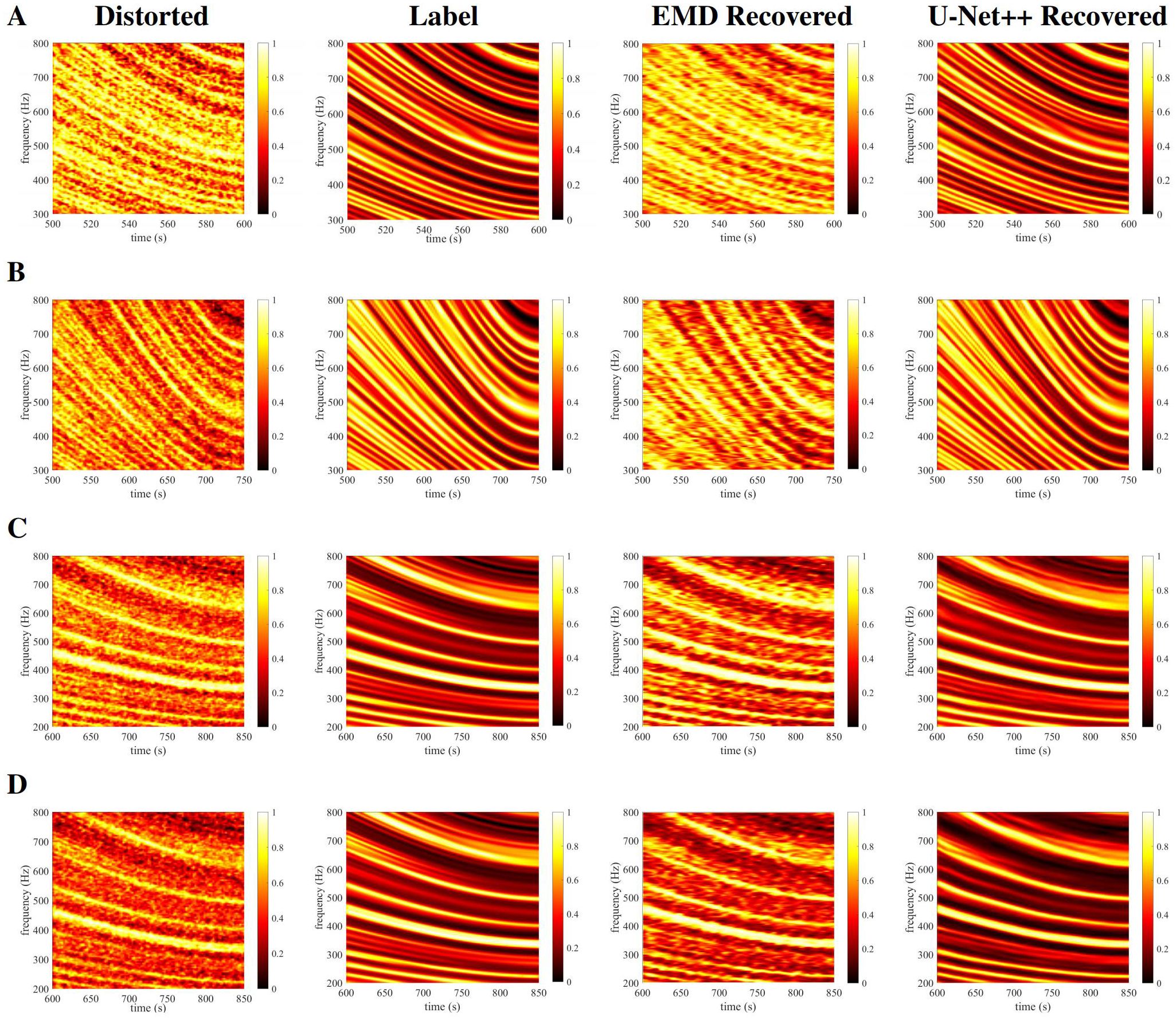
Figure 6. Simulated LOFARgrams with normalized intensity and the recovery results. (A) t_CPA = 610s, r_CPA = 2km, v = 20m/s, z_r = 20m z_s = 20m, SNR = −20dB, SSP is Yellow Sea’s January data; (B) t_CPA = 755s, r_CPA = 1.2km, v = 10m/s, z_r = 20m z_s = 20m, SNR = −20dB, SSP is Yellow Sea’s March data; (C) t_CPA = 870s, r_CPA = 1.5km, v = 5m/s, z_r = 20m z_s = 20m, SNR = −20dB, SSP is Yellow Sea’s June data; (D) The ship noise model uses the traditional sinusoidal model, with other parameters consistent with (C).

4.2 U-Net++ network architecture

The U-Net neural network is widely utilized in the field of image processing (Wang et al., 2019) and has been proven effective for image preprocessing (Reymann et al., 2019; Zhang et al., 2022). Previous research has demonstrated that by training U-Net models, it is possible to successfully recover images that have been affected by acoustic interference striations (Li et al., 2020). Compared to the traditional U-Net, U-Net++ introduces significant upgrades and improvements. U-Net++ employs a nested U-shaped architecture and dense connectivity design to optimally capture image information, enhancing feature extraction capabilities (Ajwad and Rafid, 2023). This facilitates the effective propagation and integration of features across various levels, enabling the restoration of cleaner and clearer images. Additionally, U-Net++ calculates the loss function at multiple positions, demonstrating superior efficacy in practical applications.

Figure 7 presents the preprocessing process of LOFARgrams using U-Net++, trained based on the forward model. The forward model generates the dataset for training the neural network, with a 4:1 split between the training and testing sets. In this model, the acoustic field component h(ω), represented by the channel transmission function, simulates ideal, noise-free LOFARgrams, which serve as labels for the neural network. Distorted LOFARgrams are used as input, and the neural network recovers low-quality LOFARgrams based on the learned labels. The output is high-quality LOFARgrams, which are noise-reduced channel transmission function images. Similarly, measured ship noise LOFARgrams can be input into the trained U-Net++ model. This still improves the LOFARgrams’ quality and restores the channel transmission function images.

Figure 7

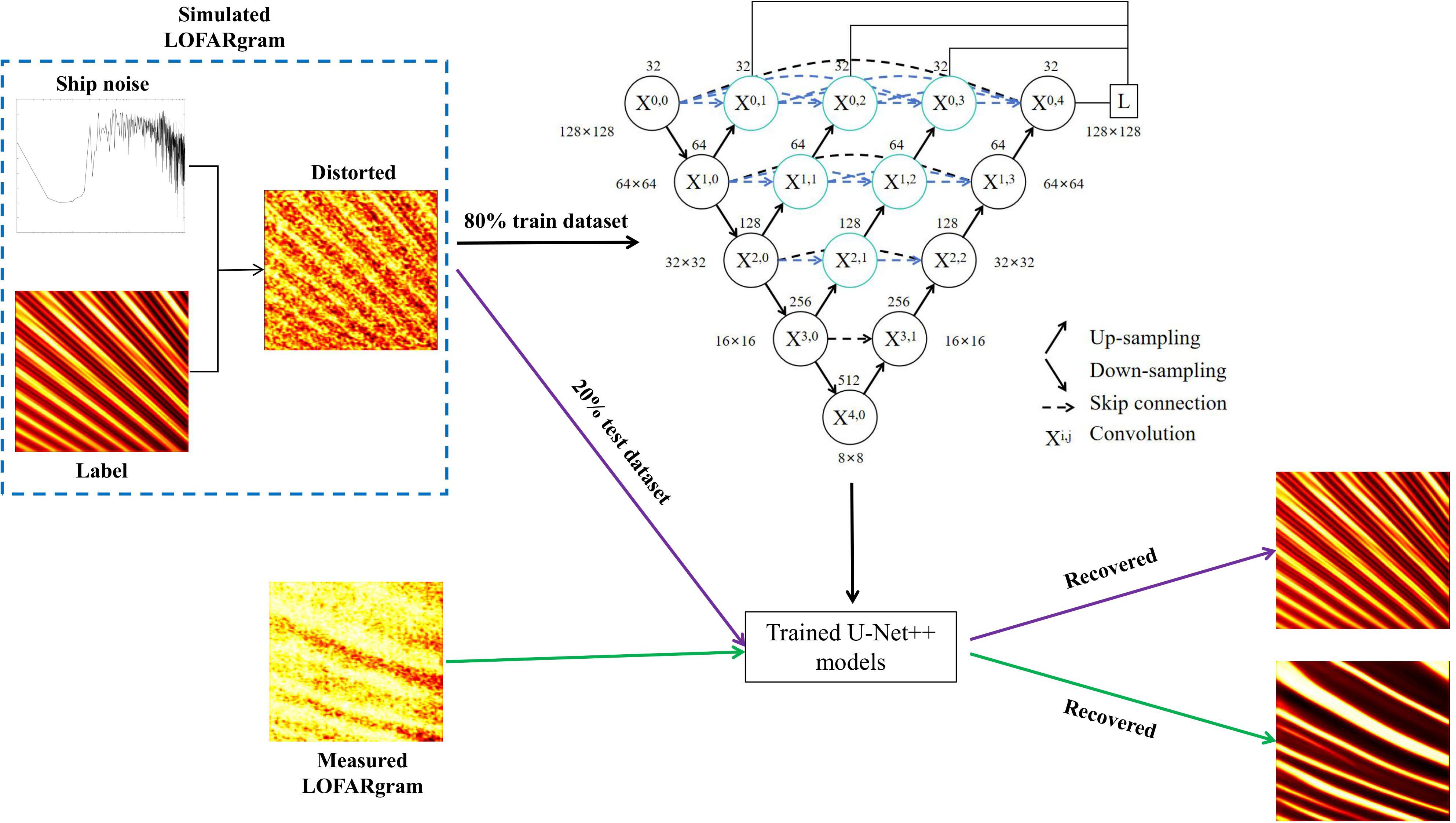
Figure 7. U-Net++ trained with the forward model for LOFARgrams preprocessing diagram.

4.3 Dataset for U-Net++

The parameter settings for the simulation dataset in this study are primarily focused on shallow sea areas. Shallow seas are major zones of human activity, holding significant ecological, economic, and social value, and are also key regions for national defense. When setting the ocean environment parameters for the dataset, it is essential to consider that hydrographic parameters such as temperature, salinity, density, and sound speed can change significantly with the seasons. Additionally, the slope of the seabed may affect sound wave propagation, and the depth and speed of the target’s movement in real scenarios must be taken into account. Therefore, to ensure the accuracy of simulation and analysis, the ocean environment parameters need to comprehensively consider hydrographic data, seabed topography, and target movement parameters.

In this study, hydrographic data are selected from the Argo dataset (Wong et al., 2020), specifically the sound speed profile data of the Yellow Sea from January to December. For seabed topography, both sloping and flat seabeds are considered. The speed range of surface ships generally varies from 5 m/s to 25 m/s. For surface ships, sonar and other acoustic equipment are usually installed at the bottom or lower part of the hull. Conventional sonar equipment is typically at depths between a few meters to several tens of meters, while the depth for warships using towed sonar arrays can be deeper, the selected source depth in this study is from 5m to 50m. The depth range of shallow sea areas is generally from 20m to 50m. Detailed parameters are shown in Table 1. According to the parameters in Table 1, a total of 20,000 LOFARgrams were simulated.

Table 1

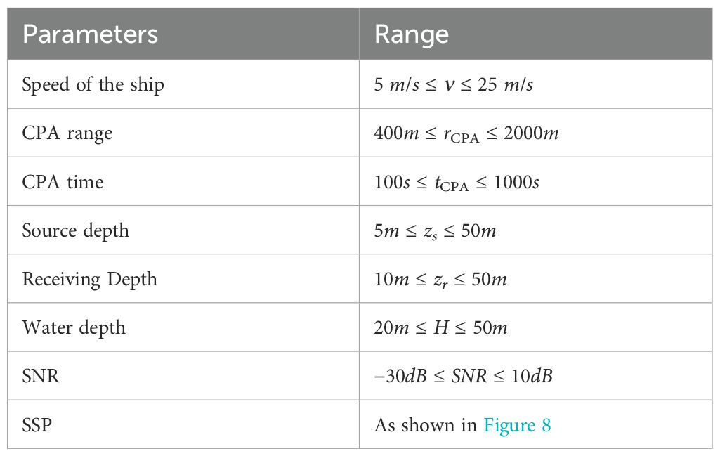
Table 1. Simulation parameters.

Figure 8

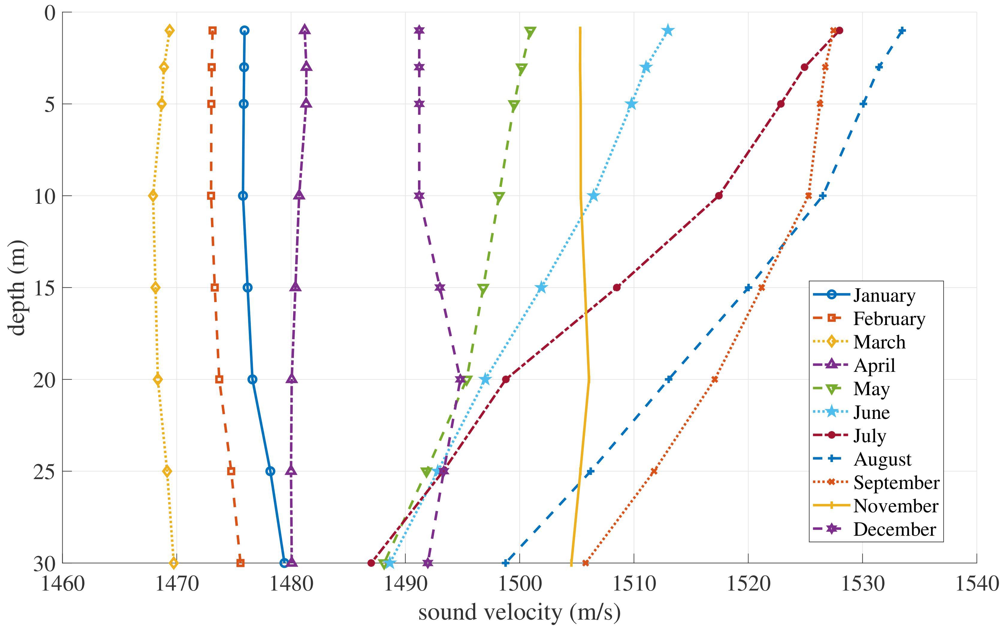
Figure 8. Monthly sound speed profiles in the Yellow Sea for 2015.

4.4 U-Net++ preprocessing results

4.4.1 Simulated LOFARgram preprocessing results

We employ the forward model to generate a dataset for training the U-Net++ model to recover low-quality LOFARgrams. In Figure 6, lines A, B, and C represent LOFARgrams simulated by the forward model using sound velocity profiles from January, March, and May in the Yellow Sea, with SNR = -20, z_s = 20m, z_r = 20m, and ship speeds of 20 m/s, 5 m/s, and 10 m/s, respectively. Line D shows the LOFARgram generated using the traditional sine model (Zhengyao and Yipeng, 2005) for ship noise simulation, with the same parameters as C. The “Distorted” column represents low-quality LOFARgrams, while the “Label” column represents clear LOFARgrams without noise interference, which is the target for the neural network recovery. “EMD Recovered” column shows the LOFARgram after processing with the EMD method, and “U-Net++ Recovered” column shows the LOFARgram after processing with the U-Net++ method. The results indicate that the EMD method provides some recovery, but U-Net++ demonstrates significantly better recovery performance, including the ability to recover LOFARgrams from traditional sine model ship noise, showing excellent scalability.

4.4.2 Measured LOFARgram preprocessing results

To further evaluate the feasibility of U-Net++ trained based on the forward model in practical applications, we performed a restoration of the LOFARgrams based on the measured data.

On June 18, 2021, we conducted a boat noise propagation experiment near Big Gong Island and Little Gong Island in Qingdao, China. During the movement of the target vessel, the Automatic Identification System (AIS) recorded the GPS positions of both the boat and the buoy, as shown in the Figure 9. The blue dots represent the boat’s trajectory, and the red star indicate the locations of the buoy. We selected a portion of the data before the CPA (orange squares) and applied Short-Time Fourier Transform (STFT) to convert the raw signals recorded by the hydrophones into LOFARgrams, as shown in the Figure 10 “Measured”. The “EMD Recovered” and “U-Net++ Recovered” show the results of preprocessing the measured LOFARgrams using the EMD and U-Net++ methods, respectively. It can be seen that the EMD method does not provide good restoration, while U-Net++ still shows promising results, further confirming the reliability of the forward model.

Figure 9

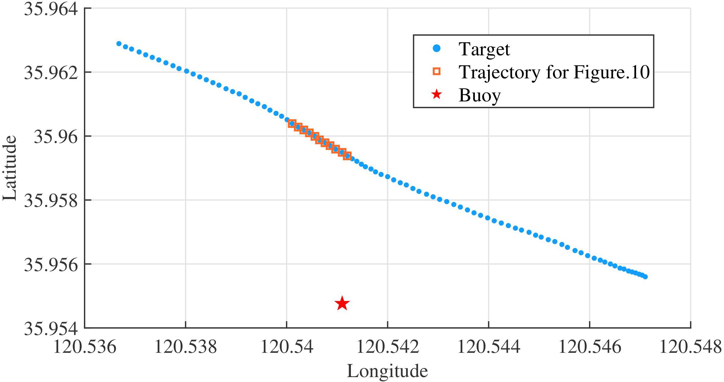
Figure 9. The GPS trajectories of the target and buoys.

Figure 10

Figure 10. Measured LOFARgrams with normalized intensity. (Measured) LOFARgrams before preprocessing enhancement. (EMD Recovered) LOFARgrams after EMD preprocessing enhancement. (U-Net++ Recovered) LOFARgrams after U-Net++ preprocessing enhancement.

The results in Figures 6 and 10 suggest that U-Net++ performs well in restoring LOFARgrams. To quantitatively assess the restoration performance of both the EMD and U-Net++ methods, we introduced the CPA parameter estimation algorithm for further analysis.

5 CPA parameter estimation

U-Net++, as an advanced deep learning model, has demonstrated its excellent performance in image restoration tasks. However, for the restoration of LOFARgrams, relying solely on visual inspection to judge the quality of restoration is insufficient. Therefore, we need more scientific and quantitative evaluation methods.

5.1 CPA parameter estimation algorithm

This section employs the CPA parameter estimation algorithm to analyze the restoration performance of the U-Net++ model. The evaluation algorithm primarily extracts the CPA parameters of the target trajectory, denoted as ${\tau }_i=t_{\mathrm{C}\mathrm{P}\mathrm{A}}$ and $b_i=r_{\mathrm{C}\mathrm{P}\mathrm{A}}/v$, through LOFARgrams, as illustrated in Figure 11.

Figure 11

Figure 11. CPA parameter estimation algorithm.

Firstly, determine the search range for CPA parameters ${\tau }_i$ and $b_i$.

$\begin{array}{ll}f=f_0{\left[1+{\left(\frac{t-{\tau }_i}{b_i}\right)}^2\right]}^{\frac{\beta }{2}},& (15)\end{array}$

where $f_0$ is the frequency value at the time of CPA, selected according to the frequency axis in the LOFARgram, β is the waveguide invariant (β = 1).

Estimate the target CPA parameters using the following form of cost function

$\begin{array}{ll}H({\tau }_i,b_i)=\sum _{f_0}\frac{{\left({\int }_{L}I(f,t)ds\right)}^2}{{\int }_{L}I(f,t)ds},& (16)\end{array}$

the curve L in the formula represents a family of curves as expressed by Equation 7. The search value that maximizes Equation 8 is the estimated value of the target CPA parameters.

To facilitate the presentation of the processing effect of our algorithm, we define the approximation ratio

R as

$\begin{array}{ll}R=1-\frac{\sqrt{{(x-x_t)}^2 + {(y-y_t)}^2}}{\sqrt{x^2 + y^2}},& (17)\end{array}$

where $(x,y)$ represents the CPA coordinates and $(x_t,y_t)$ corresponds to the true CPA values.

5.2 CPA parameter estimation results

Figure 12 presents the predicted results of the CPA parameter estimation algorithm for the simulated LOFARgram in Figure 6. Triangles represent the true values of the target CPA points, while circles indicate the predicted values. It can be observed that the predictions for the low-quality LOFARgrams in the “distorted” column exhibit a significant deviation from the true values. The EMD method do not result in a significant improvement in the CPA prediction accuracy of LOFARgrams. However, the accuracy of CPA prediction shows a notable improvement after preprocessing LOFARgrams using U-Net++. Similarly, we also applied the algorithm to predict the CPA for the measured LOFARgram corresponding to Figure 10, with the results shown in Figure 13. The results indicate that U-Net++ preprocessing is equally effective for measured LOFARgrams. The prediction range is narrowed, and the predicted values are closer to the true CPA values, demonstrating the strong generalization and effectiveness of U-Net++ preprocessing.

Figure 12

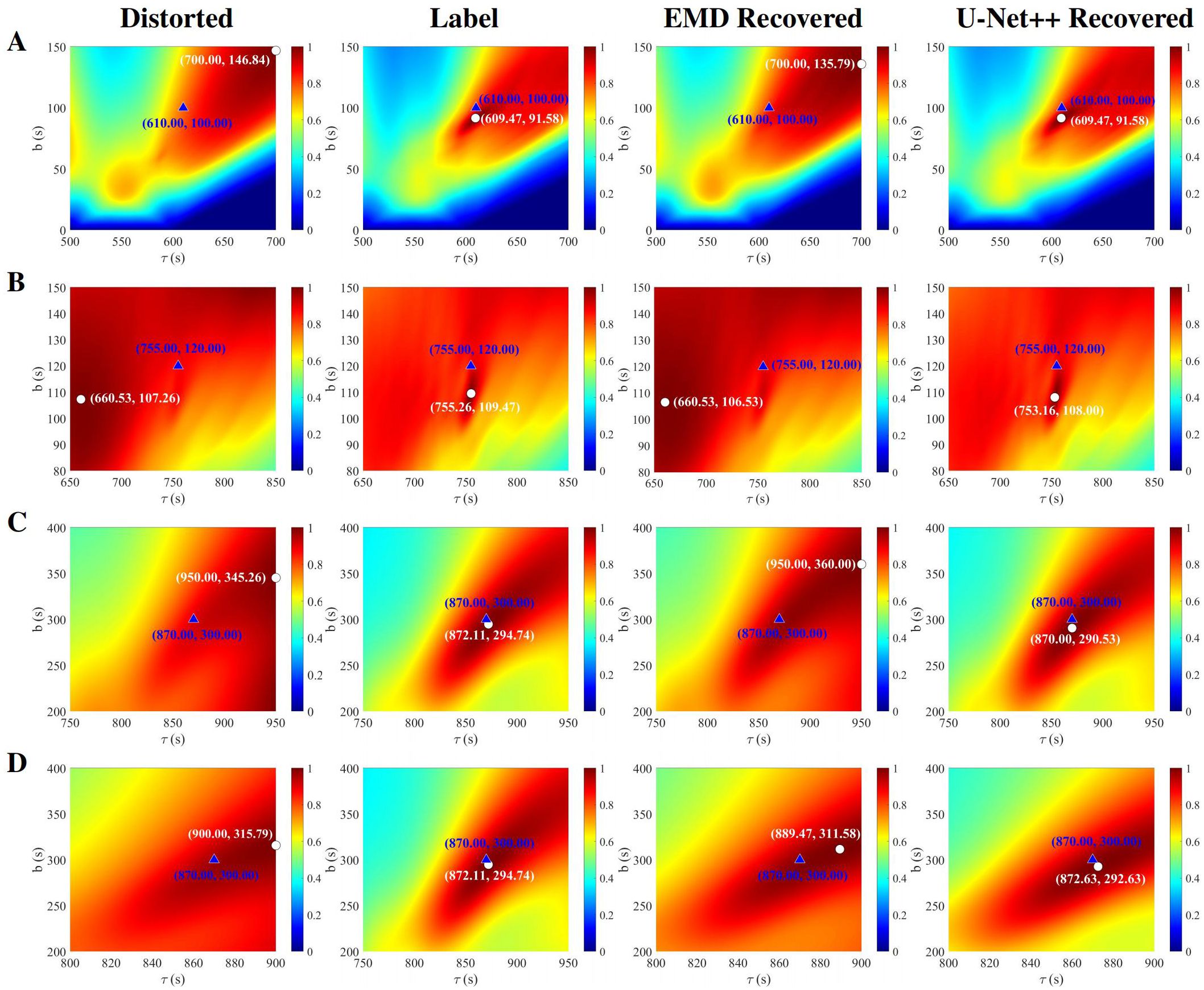
Figure 12. Results of applying the CPA parameter estimation algorithm to the LOFARgrams before and after preprocessing in Figure 6.

Figure 13

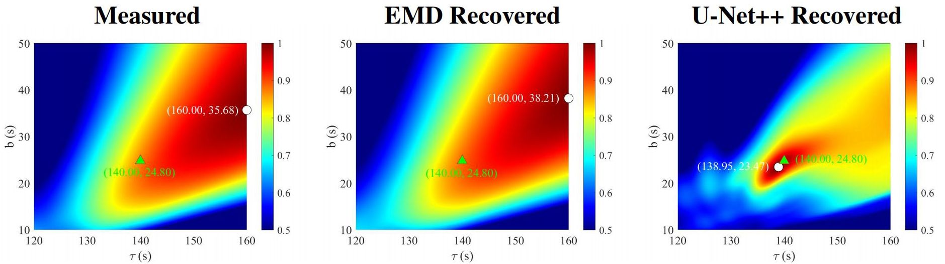
Figure 13. Results of applying the CPA parameter estimation algorithm to the measured LOFARgrams before and after preprocessing in Figure 10. (Measured) Measured LOFARgram prediction results. (EMD Recovered) The predicted results of the measured LOFARgram after EMD processing. (U-Net++ Recovered) The predicted results of the measured gram after U-Net++ processing.

To clearly demonstrate the performance of different processing methods, we quantitatively present the true CPA values (CPA_ture) of the A, B, C, D and measured LOFARgrams in Table 2, along with the predicted results and approximation ratios (R) obtained using the CPA estimation algorithm for the label, distorted, EMD-recovered and U-Net++-processed images. From the approximation ratio (R), it is evident that the EMD processing method both improves and disrupts the LOFARgram predictions, though the effects are not significant. In contrast, the predicted approximation ratio for the U-Net++-processed images closely matches that of the label, which sufficiently demonstrates the feasibility of using a neural network model trained on the forward model to recover low-quality LOFARgrams.

Table 2

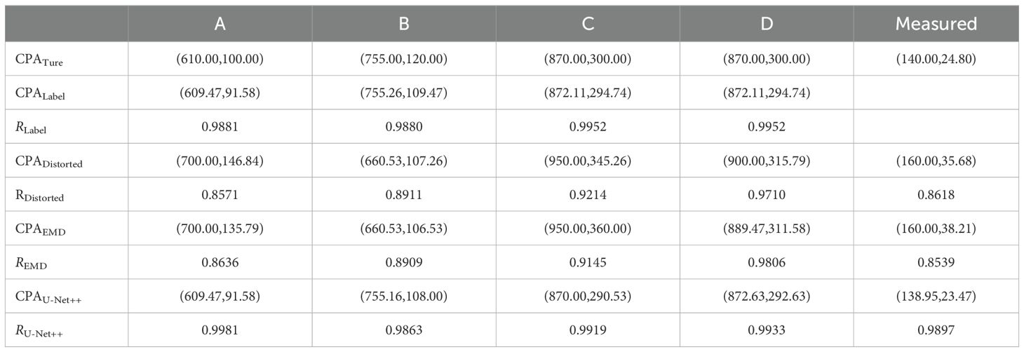
Table 2. Prediction results and approximation ratio.

6 Conclusion

We employs the U-Net++ neural network to preprocess low-quality LOFARgrams, demonstrating effective recovery results. The collection of measured data is costly and time-consuming, resulting in insufficient data for training the neural network. To address this limitation, we propose an innovative forward model to simulate LOFARgrams. The forward model consists of three components: ship noise, a sound field model, and Gaussian white noise. Ship noise is simulated using quasi-periodic randomly distributed explosive cosine pulses, while the sound field model is constructed using the KRAKEN normal mode model, and then Gaussian white noise is added. By continuously adjusting the parameters of the forward model, LOFARgrams that closely resemble actual data can be generated, overcoming the limitation of insufficient measured LOFARgrams. The U-Net++ neural network, trained based on a forward model, demonstrates superior recovery performance for both simulated and measured LOFARgrams, significantly enhancing the quality and usability of LOFARgrams.

Additionally, we introduce a CPA parameter estimation algorithm to quantitatively assess the effectiveness of the U-Net++ network’s recovery performance. The results show that the predicted CPA values of the U-Net++-processed LOFARgrams closely match the true CPA values, with a correlation exceeding 0.99, significantly reducing the prediction range and enhancing the accuracy of target motion parameter estimation.

This research provides a reliable method for simulating and recovering LOFARgrams, offering promising prospects for marine monitoring and analysis. Future work will focus on further optimizing various strategies and exploring their potential applications in different scenarios.

Data availability statement

The raw data supporting the conclusions of this article will be made available by the authors, without undue reservation.

Author contributions

DP: Conceptualization, Investigation, Methodology, Software, Validation, Writing – original draft, Writing – review & editing. XX: Software, Validation, Writing – original draft, Writing – review & editing. WS: Conceptualization, Data curation, Formal Analysis, Funding acquisition, Investigation, Methodology, Project administration, Resources, Software, Supervision, Validation, Writing – original draft, Writing – review & editing. DG: Data curation, Investigation, Writing – review & editing.

Funding

The author(s) declare financial support was received for the research, authorship, and/or publication of this article. This paper is supported by the National Natural Science Foundation of China (Grant No. 12004359).

Conflict of interest

The authors declare that the research was conducted in the absence of any commercial or financial relationships that could be construed as a potential conflict of interest.

Generative AI statement

The author(s) declare that no Generative AI was used in the creation of this manuscript.

Publisher’s note

All claims expressed in this article are solely those of the authors and do not necessarily represent those of their affiliated organizations, or those of the publisher, the editors and the reviewers. Any product that may be evaluated in this article, or claim that may be made by its manufacturer, is not guaranteed or endorsed by the publisher.

References

Ajwad A. J., Rafid S. T. S. (2023). “Enhancing facial image clarity: Deblurring gaussian blur with unet++ architecture,” In IEEE International Conference on Computer and Information Technology (ICCIT). 1–4. doi: 10.1109/ICCIT60459.2023.10441021

Crossref Full Text | Google Scholar

Chen J., Han B., Ma X., Zhang J. (2021). Underwater target recognition based on multi-decision lofar spectrum enhancement: A deep-learning approach. Future Internet 13, 265. doi: 10.3390/fi13100265

Crossref Full Text | Google Scholar

Chuprov S., Brekhovskikh L. (1982). Interference structure of a sound field in a layered ocean. Ocean Acoust. Curr. State, 71–91.

Google Scholar

Guo D., Gao D., Chen Z., Li Y., Zhao X., Song W., et al. (2023). Classification of inbound and outbound ships using convolutional neural networks. Front. Mar. Sci. 10, 1151817. doi: 10.3389/fmars.2023.1151817

Crossref Full Text | Google Scholar

Han Y., Li Y., Liu Q., Ma Y. (2020). Deeplofargram: A deep learning based fluctuating dim frequency line detection and recovery. J. Acoust. Soc. America 148, 2182–2194. doi: 10.1121/10.0002172

PubMed Abstract | Crossref Full Text | Google Scholar

Huang N. E., Shen Z., Long S. R., Wu M. C., Shih H. H., Zheng Q., et al. (1998). The empirical mode decomposition and the hilbert spectrum for nonlinear and non-stationary time series analysis. Proc. R. Soc. London Ser. A: Mathematical Phys. Eng. Sci. 454, 903–995. doi: 10.1098/rspa.1998.0193

PubMed Abstract | Crossref Full Text | Google Scholar

Jun-Ping S., Jun Y., Jian-Heng L., Guo-Jian J., Xue-Juan Y., Peng-Fei J. (2016). Theoretical model and simulation of ship underwater radiated noise. Acta Physica Sin. 65, 124301-1-10. doi: 10.7498/aps.65.124301

Crossref Full Text | Google Scholar

Li J., Han G., Zhou D., Tang K., Han Q. (2016). “Target motion parameter estimation for lofargrams based on waveguide invariants,” Underwater Acoustics and Ocean Dynamics. 85–92. doi: 10.1007/978-981-10-2422-1_12

Crossref Full Text | Google Scholar

Li X., Song W., Gao D., Gao W., Wang H. (2020). Training a u-net based on a random mode-coupling matrix model to recover acoustic interference striations. J. Acoust. Soc. America 147, EL363–EL369. doi: 10.1121/10.0001125

PubMed Abstract | Crossref Full Text | Google Scholar

Liu Y., Lv Y., Lv T., Wei Y., Liu X. (2019). “Simulation of ship-radiated noise based on shallow marine environment,” In IEEE International Conference on Signal, Information and Data Processing (ICSIDP). 1–5. doi: 10.1109/ICSIDP47821.2019.9173032

Crossref Full Text | Google Scholar

Peng C., Yang L., Jiang X., Song Y. (2019). “Design of a ship radiated noise model and its application to feature extraction based on winger’s higher-order spectrum,” In IEEE Advanced Information Technology, Electronic and Automation Control Conference (IAEAC). 582–587. doi: 10.1109/IAEAC47372.2019.8997718

Crossref Full Text | Google Scholar

Porter M. B. (1992). The kraken normal mode program. Washington,D.C.: Naval Research Laboratory.

Google Scholar

Reymann M. P., Würfl T., Ritt P., Stimpel B., Cachovan M., Vija A. H., et al. (2019). “U-net for spect image denoising,” In IEEE Nuclear Science Symposium and Medical Imaging Conference (NSS/MIC). 1–2. doi: 10.1109/NSS/MIC42101.2019.9059879

Crossref Full Text | Google Scholar

Rouseff D., Leigh C. (2002). “Using the waveguide invariant to analyze lofargrams,” In IEEE OCEANS '02 MTS. vol. 4. (IEEE), 2239–2243. doi: 10.1109/OCEANS.2002.1191978

Crossref Full Text | Google Scholar

Song W., Gao D., Li X., Kang D., Li Y. (2022). Waveguide invariant in a gradual range-and azimuth-varying waveguide. JASA Express Lett. 2 (5), 056002. doi: 10.1121/10.0010489

PubMed Abstract | Crossref Full Text | Google Scholar

Wang Y., Zhu X., Zhao Y., Wang P., Ma J. (2019). “Enhancement of low-light image based on wavelet u-net,” in Journal of Physics: Conference Series, Vol. 1345. 022030 (IOP Publishing).

Google Scholar

Wong A. P., Wijffels S. E., Riser S. C., Pouliquen S., Hosoda S., Roemmich D., et al. (2020). Argo data 1999–2019: Two million temperature-salinity profiles and subsurface velocity observations from a global array of profiling floats. Front. Mar. Sci. 7, 700. doi: 10.3389/fmars.2020.00700

Crossref Full Text | Google Scholar

Yang T. (2003). Beam intensity striations and applications. J. Acoust. Soc. America 113, 1342–1352. doi: 10.1121/1.1534604

PubMed Abstract | Crossref Full Text | Google Scholar

Zhang W., Li H., Sun H., Bai Y. (2022). “Dehazing network based on u-net structure and residual block,” In IEEE Chinese Control Conference (CCC. 6576–6581. doi: 10.23919/CCC55666.2022.9902049

Crossref Full Text | Google Scholar

Zhao X.-W., Chen Z., Wang Z.-W., Liu Z.-G., Wang M.-R., Liang Q. (2022). “Modeling and simulation of passive sonar signal under channel conditions,” In IEEE International Conference on Information Communication and Signal Processing (ICICSP). 555–559. doi: 10.1109/ICICSP55539.2022.10050567

Crossref Full Text | Google Scholar

Zheng Y., JIANG B., Gang Y. (2020). “Simulation of dynamic ship radiated noise signal,” In IEEE International Conference on Signal Processing (ICSP), 636–639. doi: 10.1109/ICSP48669.2020.9320983

Crossref Full Text | Google Scholar

Zhengyao H., Yipeng Z. (2005). Modeling and simulation research of ship-radiated noise. Audio Eng. 12, 52–56. doi: 10.2991/iiicec-15.2015.372

Crossref Full Text | Google Scholar

Zhou Z., Rahman Siddiquee M. M., Tajbakhsh N., Liang J. (2018). “Unet++: A nested u-net architecture for medical image segmentation,” Deep Learn Med Image Anal Multimodal Learn Clin Decis Support, 3–11. doi: 10.1007/978-3-030-00889-5_1

PubMed Abstract | Crossref Full Text | Google Scholar