An estimation method of sound speed profile based on grouped dilated convolution informer model

Introduction: The accurate determination of the ocean sound speed profile (SSP) is essential for oceanographic research and marine engineering. Traditional methods for acquiring SSP data are often time-consuming and costly. Machine learning techniques provide a more efficient alternative for SSP inversion, effectively addressing the limitations of conventional approaches.

Methods: This study proposes a novel SSP inversion model based on a grouped dilated convolution (GDC) Informer architecture. By replacing the standard one-dimensional convolution in the Informer model with GDC, the proposed model expands its receptive field and improves computational efficiency. The model was trained using Argo profile data from 2008 to 2017, incorporating empirical orthogonal function (EOF) decomposition data, geographic location, temporal information, and historical SSP data, enabling SSP inversion across diverse regions and time periods.

Results: The model’s performance was evaluated using mean absolute error (MAE), root mean square error (RMSE) and mean absolute percentage error (MAPE) metrics. Experimental results demonstrate that the Informer-GDC model achieves evaluation metrics of 0.355 m/s and 0.611 m/s for MAE, 0.241 m/s and 0.394 m/s for RMSE, and 0.018% and 0.025% for MAPE compared with measured data from 2018.

Discussion: Compared to the LSTM and Informer models, the proposed model improves MAE, RMSE, and MAPE by 46.51% and 29.66%, 51.65% and 39.28%, and 51.25% and 37.08%, respectively. These findings highlight the superior accuracy, stability, and efficiency of the Informer-GDC model, marking a significant advancement in SSP inversion methodologies.

1 Introduction

The sound speed profile (SSP) is a fundamental parameter in oceanography, marine engineering, and seabed topography studies (Liu and Jiayu, 2010). Accurate determination of SSP is crucial for various research areas (LeBlanc et al., 1980; Leroy et al., 2008; Talib et al., 2011). Traditionally, SSP observations have relied on in-situ measurements, such as sound velocity profilers (SVPs). However, deploying such equipment across large oceanic regions is both time-intensive and expensive, making large-scale monitoring impractical (Heidemann et al., 2012; Huang et al., 2020). To address these challenges, researchers have proposed indirect SSP inversion methods (DeSanto, 1984), among which machine learning-based approaches have emerged as particularly representative. These methods analyze historical data to estimate SSP, significantly reducing costs and improving scalability.

Recent studies have demonstrated that machine learning-based methods not only enhance SSP prediction accuracy but also enable real-time monitoring and high-resolution data analysis, making them highly applicable for large-scale ocean studies and environmental monitoring (Bianco et al., 2019; Li et al., 2022). Notably, machine learning models such as artificial neural networks (ANN), long short-term memory (LSTM) networks, and self-organizing maps (SOM) have shown great potential for SSP inversion (Jain and Ali, 2006; Feng et al., 2021). For example, Li et al. utilized ANN models to invert SSP with promising results, laying a foundation for subsequent ANN-based studies (Li et al., 2022). Huang et al. combined ANN with ray theory to invert SSP (Huang et al., 2018). Similarly, Huang et al. applied clustering analysis and feedforward neural networks to construct a multi-task model for SSP inversion (Huang et al., 2023). Hou et al. developed a hierarchical approach by stratifying SSP data and employing LSTM networks to construct SSP models (Hou et al., 2020). Numerous other studies have demonstrated the effectiveness of machine learning in achieving high SSP inversion accuracy (Jain and Ali, 2006; Huang et al., 2012; Ballard et al., 2014; Yang et al., 2020; Yuan et al., 2023; Huang et al., 2024). These models, trained on large historical datasets, have proven capable of providing high-accuracy predictions. However, challenges remain, including overfitting, the requirement for extensive training data, and computational complexities in processing high-dimensional nonlinear data.

To reduce computational complexity, Davis (1976) demonstrated that empirical orthogonal function (EOF) decomposition effectively extracts sound speed features. By combining the first mmm EOF modes with the mean SSP, SSP characteristics can be accurately represented, providing a theoretical foundation for subsequent inversion studies. J.C. Park integrated EOF decomposition with multilayer perceptron neural networks for SSP inversion. Li et al. developed a model combining SOM and EOF-based regression (sEOF-R) for SSP inversion (Li et al., 2021). Bianco et al. applied sparse dictionary learning to optimize SSP representation and integrated EOF decomposition for inversion (Bianco and Gerstoft, 2017; Castro-Correa et al., 2022). Feng et al. built an SSP inversion model combining EOF decomposition with MLR, SVM, and XGBoost for Argo data inversion and prediction (Feng et al., 2024). Other researchers have also employed EOF decomposition with BPNN and LSTM (Wang et al., 2020; Piao et al., 2023). While these methods have yielded promising results, models like BPNN and SOM lack the flexibility of modern architectures, whereas LSTM and deep networks require substantial training data and computational resources, potentially limiting their application in data-sparse environments.

Informer model, which utilizes a probabilistic sparse attention mechanism, effectively addresses the challenges associated with long-sequence SSP inversion. It demonstrates superior prediction accuracy compared to alternative models by analyzing the intrinsic relationships within the dataset (Zhou et al., 2021; Yang et al., 2022; Tong et al., 2024). This study introduces Informer model to the domain of SSP inversion and presents the following contributions:

1. The self-attention extraction process within the encoder module of Informer model has been improved by replacing traditional convolution with grouped dilated convolution (GDC). This enhancement enables the model to prioritize the extraction of SSP features, thereby augmenting its capability for inverse operations.

2. SSP data were extracted from the Argo dataset and subsequently decomposed using EOF. The training dataset includes the following variables: temperature, depth, salinity, EOF components, latitude, longitude, time, and historical SSP. The results of a series of experiments indicate that Informer-GDC model exhibits superior performance compared to both LSTM and Informer models, particularly in terms of inversion accuracy and stability.

In summary, the structure of this paper is organized as follows: Section 2 provides an overview of the relevant algorithms and the unique process of SSP inversion. Section 3 outlines the data sources employed in the experimental procedure and offers a comprehensive description of the input dataset. Section 4 delivers a thorough analysis of the experimental results. Finally, Section 5 synthesizes the results and presents novel insights into SSP inversion.

2 Materials and methods

2.1 EOF representation of SSP

The complexity of marine ecosystems renders the use of basic mathematical models insufficient for accurately representing the characteristics of SSP. To mitigate the complexity associated with SSP, the empirical orthogonal decomposition method is employed to analyze sound speed data. Typically, the first five mode vectors (i.e., those that account for a cumulative contribution rate exceeding 95%) are selected to characterize SSP within a given region (Smith et al., 1996). SSP for a specific region can be articulated using the first m feature vectors as follows:

$\begin{array}{ll}\begin{array}{c}\mathit{C}\mathit{z}\mathbf{=}{\mathit{C}}_{\mathbf{0}}\mathbf{+}\mathbf{\sum }_{\mathit{i}\mathbf{=}\mathbf{1}}^{\mathit{m}}{\mathit{\alpha }}_{\mathit{i}}{\mathit{f}}_{\mathit{i}}(\mathit{z})\end{array}& (1)\end{array}$

where z represents depth; ${\mathit{C}}_{\mathbf{0}}$ represents the mean SSP; ${\mathit{\alpha }}_{\mathit{i}}$ represents the coefficients of the EOF modes for SSP; and ${\mathit{f}}_{\mathit{i}}(\mathit{z})$ represents EOF.

2.2 Informer model

Informer model is a long-sequence forecasting framework that has been introduced in recent years. Its primary advantage lies in its ability to effectively identify and elucidate the relationships among features associated with different data points. Informer model represents an advancement over Transformer model, sharing a similar structural configuration. The encoder integrates ProbSparse self-attention and convolutional pooling layers, which enhance the computational efficiency of the model and address the challenges associated with high computational complexity and inefficiencies resulting from excessively deep attention stacks. Furthermore, the decoder generates predictions in a single step, significantly expediting the long-sequence forecasting process while avoiding the error accumulation that is typically associated with multi-step predictions.

ProbSparse self-attention is formulated utilizing the query matrix Q, the key matrix K, and the value matrix V. In contrast to the conventional self-attention mechanism, which requires a quadratic complexity $O(L_Q{L}_K)$ for the computation of dot products, ProbSparse self-attention eliminates the need for this additional calculation. This methodology improves computational efficiency by focusing on dot products that exhibit high contribution rates while disregarding those with low contribution rates. The computation is executed as follows:

$\begin{array}{ll}\begin{array}{c}\mathit{A}\mathit{t}\mathit{t}\mathit{e}\mathit{n}\mathit{t}\mathit{i}\mathit{o}\mathit{n}\mathit{Q}\mathbf{,}\mathit{K}\mathbf{,}\mathit{V}\mathbf{=}\mathit{S}\mathit{o}\mathit{f}\mathit{t}\mathit{m}\mathit{a}\mathit{x}(\frac{\overline{\mathit{Q}}{\mathit{K}}^{\mathit{T}}}{\sqrt{\mathit{d}}})\mathit{V}\end{array}& (2)\end{array}$

where $\overline{\mathit{Q}}$ represents the sparsified matrix of Q, which includes the sparsity measure $\mathit{M}(\mathit{Q}\mathbf{,}\mathit{K})$; V represents the value matrix; ${\mathit{K}}^{\mathit{T}}$ represents the transpose of the key matrix; d represents the input matrix; and $Softmax(\cdot )$ represents the activation function.

The distillation process reduces the length of the input sequence or matrix by half, thereby emphasizing key features. This is achieved through the utilization of pooling layers to extract these features, which subsequently generates a self-attention feature map within a more compact range. The distillation from the i-th to the (i+1)-th self-attention layer is determined as follows:

$\begin{array}{ll}\begin{array}{c}{\mathit{X}}_{\mathit{i}\mathbf{+}\mathbf{1}}^{\mathit{t}}\mathbf{=}\mathit{M}\mathit{a}\mathit{x}\mathit{P}\mathit{o}\mathit{o}\mathit{l}(\mathit{E}\mathit{L}\mathit{U}(\mathit{C}\mathit{o}\mathit{n}\mathit{c}\mathbf{1}\mathit{d}{[{\mathit{X}}_{\mathit{i}}^{\mathit{t}}]}_{\mathit{A}\mathit{B}}))\end{array}& (3)\end{array}$

where ${[{\mathit{X}}_{\mathit{i}}^{\mathit{t}}]}_{\mathit{A}\mathit{B}}$ represents the attention module; $\mathit{C}\mathit{o}\mathit{n}\mathit{c}\mathbf{1}\mathit{d}(\mathbf{\cdot })$ represents the one-dimensional convolution operation along the depth sequence; ELU represents the activation function; and $\mathit{M}\mathit{a}\mathit{x}\mathit{P}\mathit{o}\mathit{o}\mathit{l}(\mathbf{\cdot })$ represents the max pooling layer.

The architecture of the decoder adheres to a conventional configuration, comprising two identical multi-head attention layers that are stacked in succession. This configuration generates predictions via a single-step forward operation. The output vector produced by the decoder is expressed as follows:

$\begin{array}{ll}\begin{array}{c}{\mathit{X}}_{\mathit{f}\mathit{e}\mathit{e}{\mathit{d}}_{\mathit{d}\mathit{e}}}\mathbf{=}\mathbf{C}\mathbf{o}\mathbf{n}\mathbf{c}\mathbf{a}\mathbf{t}({\mathit{X}}_{\mathit{t}\mathit{o}\mathit{k}\mathit{e}\mathit{n}}^{\mathit{t}}\mathbf{,}{\mathit{X}}_{\mathbf{0}}^{\mathit{t}})\mathbf{\in }{\mathit{R}}^{({\mathit{L}}_{\mathit{t}\mathit{o}\mathit{k}\mathit{e}\mathit{n}}\mathbf{+}{\mathit{L}}_{\mathit{y}})\mathbf{\times }{\mathit{d}}_{\mathit{m}\mathit{o}\mathit{d}\mathit{e}\mathit{l}}}\end{array}& (4)\end{array}$

where ${\mathit{X}}_{\mathit{t}\mathit{o}\mathit{k}\mathit{e}\mathit{n}}^{\mathit{t}}$ represents the start token and ${\mathit{X}}_{\mathbf{0}}^{\mathit{t}}$ represents a placeholder for the label sequence, typically set to zero. The multi-head attention mechanism in the decoder diverges from that in the encoder, with the dot product filter set to $-\infty$ for preventing autoregressive effects in the prediction data.

2.3 Informer network based on group dilated convolution

2.3.1 Group dilated convolution

Grouped convolution possesses the ability to improve the computational efficiency while keeping the parameters unchanged. Additionally, it necessitates a minimal duration to extract feature information (Jeon and Kim, 2021; Chen et al., 2022; Zhu et al., 2023). When the input size of standard convolution is G, the parameter count for grouped convolution is reduced to 1/G, thereby significantly decreasing the computational complexity of the convolutional network model. The convolution operation for each group is defined as follows:

$\begin{array}{ll}\begin{array}{c}{\mathit{x}}^{\mathit{i}}\mathbf{=}\mathit{f}({\mathit{W}}^{\mathit{i}}{\mathit{x}}^{\mathit{i}}\mathbf{+}{\mathit{\beta }}^{\mathit{i}})\mathbf{,}\mathit{i}\mathbf{=}\mathbf{1}\mathbf{\cdots }\mathit{ɡ}\end{array}& (5)\end{array}$

where $x=x^1\cup x^2\cup \cdots \cup x^g$ represents the output feature map; $W^i$ and ${\beta }^i$ represent the model parameters; and f(∙) represents the activation function.

While group convolution effectively reduces the number of parameters within a neural network, it concurrently limits the exchange of information between groups, which can lead to a decline in the network’s learning capacity and a weakened representation of features. To mitigate the adverse effects on learning capability, dilated convolution has been introduced. The primary principle of dilated convolution involves the integration of zero values (representing void information) into the standard convolution kernel. This modification serves to expand the receptive field of the convolutional network, thereby allowing the output to capture a broader spectrum of information (Chen et al., 2018; Lin et al., 2018; Xia et al., 2020). Importantly, dilation enhances the spacing of the convolution kernel without increasing the number of parameters, thereby extending the range of feature information (Wang et al., 2021). Assuming the size of the dilated convolution kernel is k and the dilation rate R, the effective kernel size K₁ can be calculated as follows:

$\begin{array}{ll}\begin{array}{c}{\mathit{K}}_{\mathbf{1}}\mathbf{=}\mathit{k}\mathbf{+}(\mathit{k}\mathbf{-}\mathbf{1})\mathbf{*}(\mathit{R}\mathbf{-}\mathbf{1})\end{array}& (6)\end{array}$

The size of the convolution kernel significantly impacts feature extraction. Different kernel sizes present varying receptive fields; smaller kernels tend to concentrate on local information, whereas larger kernels capture global information. Although there is no universally accepted standard for selecting the kernel size, this model follows the parameters developed by Jiang et al. (2019) with the aim of enhancing the receptive field without altering the number of parameters. This process is depicted in Figure 1, where the value of 580 represents the spatial features of the input data following convolution, and the value of 12 denotes the number of channels generated post-convolution. The subsequent steps to be undertaken are as follows:

Figure 1

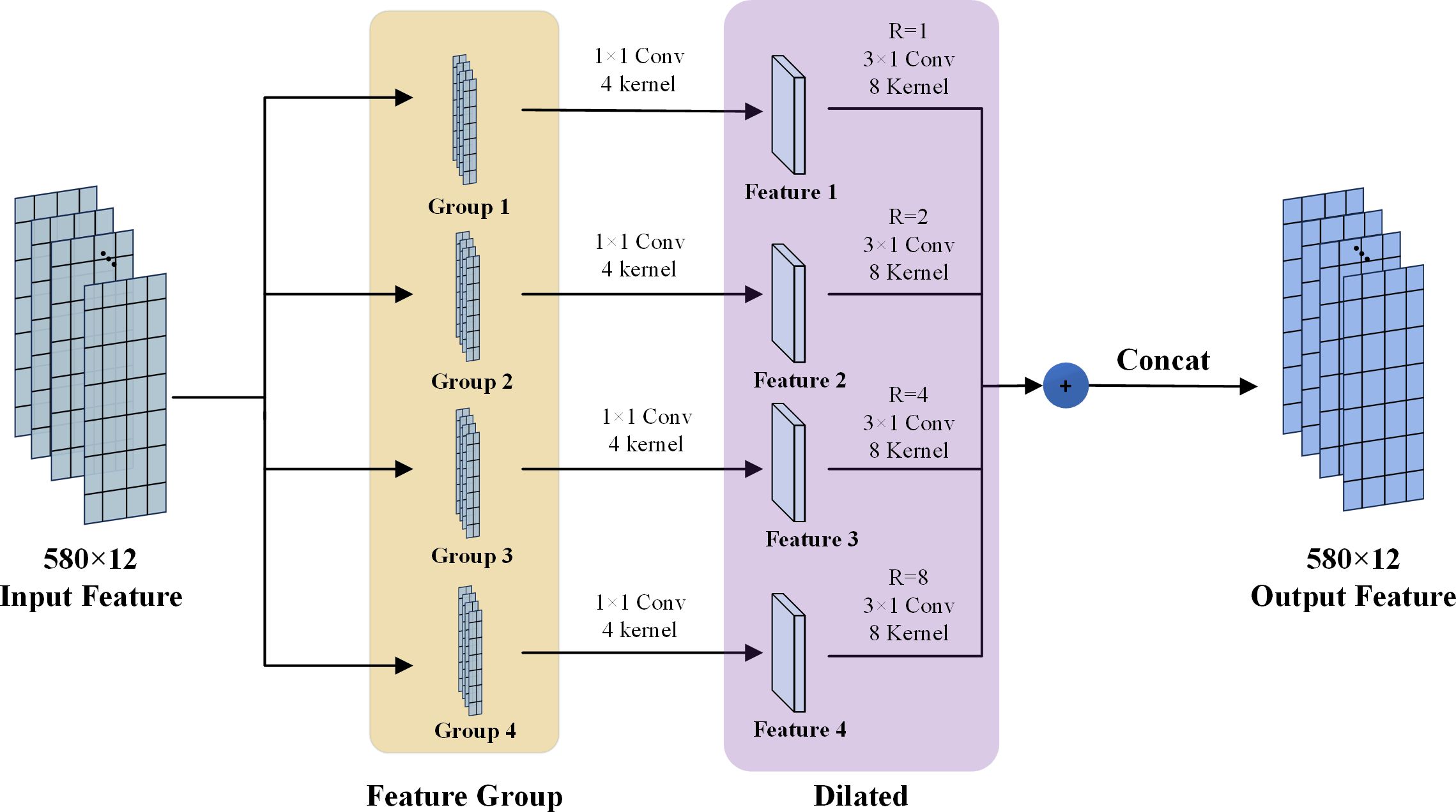
Figure 1. Group dilated convolutions process..

Step 1: The input feature map is partitioned into four feature groups, each measuring 580×3. Subsequently, these groups are processed through a convolutional layer characterized by a kernel size of 4 and a stride of 1, resulting in an output feature map of 580×3 for each group.

Step 2: The feature maps are subsequently processed through dilated convolution layers, utilizing kernel sizes of 8, a stride of 3, and dilation rates of 1, 2, 4, and 8. This process results in an output feature dimension of 580×3 for each group.

Step 3: The features obtained are concatenated across dimensions, yielding an output feature map of dimensions 580×12. To ensure the symmetry of the resulting output feature maps, the convolution kernels employed in the group of dilated convolutions are configured to be odd numbers. This configuration aids in the subsequent data stitching process. Extensive experimentation has shown that utilizing convolution kernels of odd numbers significantly enhances the capability for feature extraction.

2.3.2 Group dilated convolution informer model

The integration of ProbSparse self-attention with a convolutional module for feature map extraction, alongside the stacking of self-attention and one-dimensional convolution modules, is likely to lead to an increase in computational costs. This increase arises from a reduction in the perceptual field, which consequently results in redundant computations and a decrease in computational efficiency. This issue is particularly pronounced when handling long sequence data. To mitigate this challenge, this study proposes the implementation of grouped extended convolution as a substitute for the original convolution, with the objective of enhancing the model’s ability to identify features across a wider perceptual field.

Informer-GDC model consists of four primary components: the input layer, the encoding layer, the decoding layer, and the output layer. The input layer is primarily tasked with preprocessing SSP data, which includes calculating sound speed, selecting relevant sound speed feature quantities, and partitioning SSP dataset. The encoding and decoding layers form the core of the model, concentrating on the positional and temporal encoding of the input training data. The output layer is responsible for linking the model’s output, thereby facilitating the acquisition of inversion results and the evaluation of their accuracy.

The dataset is input into the model’s encoder and decoder, where the data undergoes an embedding process that produces modal features, depth features, and SSP features. These features are represented as follows:

$\begin{array}{ll}\begin{array}{c}\mathit{X}\mathbf{=}{\mathit{x}}_{\mathit{I}\mathit{m}\mathit{f}}\mathbf{+}{\mathit{x}}_{\mathit{T}\mathit{S}\mathit{D}}\mathbf{+}{\mathit{x}}_{\mathit{H}\mathit{S}\mathit{S}\mathit{P}}\mathbf{+}{\mathit{x}}_{\mathit{L}\mathit{o}\mathit{c}\mathit{a}\mathit{t}\mathit{i}\mathit{o}\mathit{n}}\mathbf{+}{\mathit{x}}_{\mathit{T}\mathit{i}\mathit{m}\mathit{e}}\end{array}& (7)\end{array}$

where ${\mathit{x}}_{\mathit{I}\mathit{m}\mathit{f}}$ represents the encoding of input modal data; ${\mathit{x}}_{\mathit{T}\mathit{S}\mathit{D}}$ represents the encoding of input temperature, salinity, and depth, with consideration of temperature and salinity at different depths; ${\mathit{x}}_{\mathit{H}\mathit{S}\mathit{S}\mathit{P}}$ represents the encoding of historical SSP; ${\mathit{x}}_{\mathit{L}\mathit{o}\mathit{c}\mathit{a}\mathit{t}\mathit{i}\mathit{o}\mathit{n}}$ encodes the geographical location of the SSP; and ${\mathit{x}}_{\mathit{T}\mathit{i}\mathit{m}\mathit{e}}$ represents the time at which SSP was recorded. The subsequent section illustrates the model workflow, as shown in Figure 2.

Figure 2

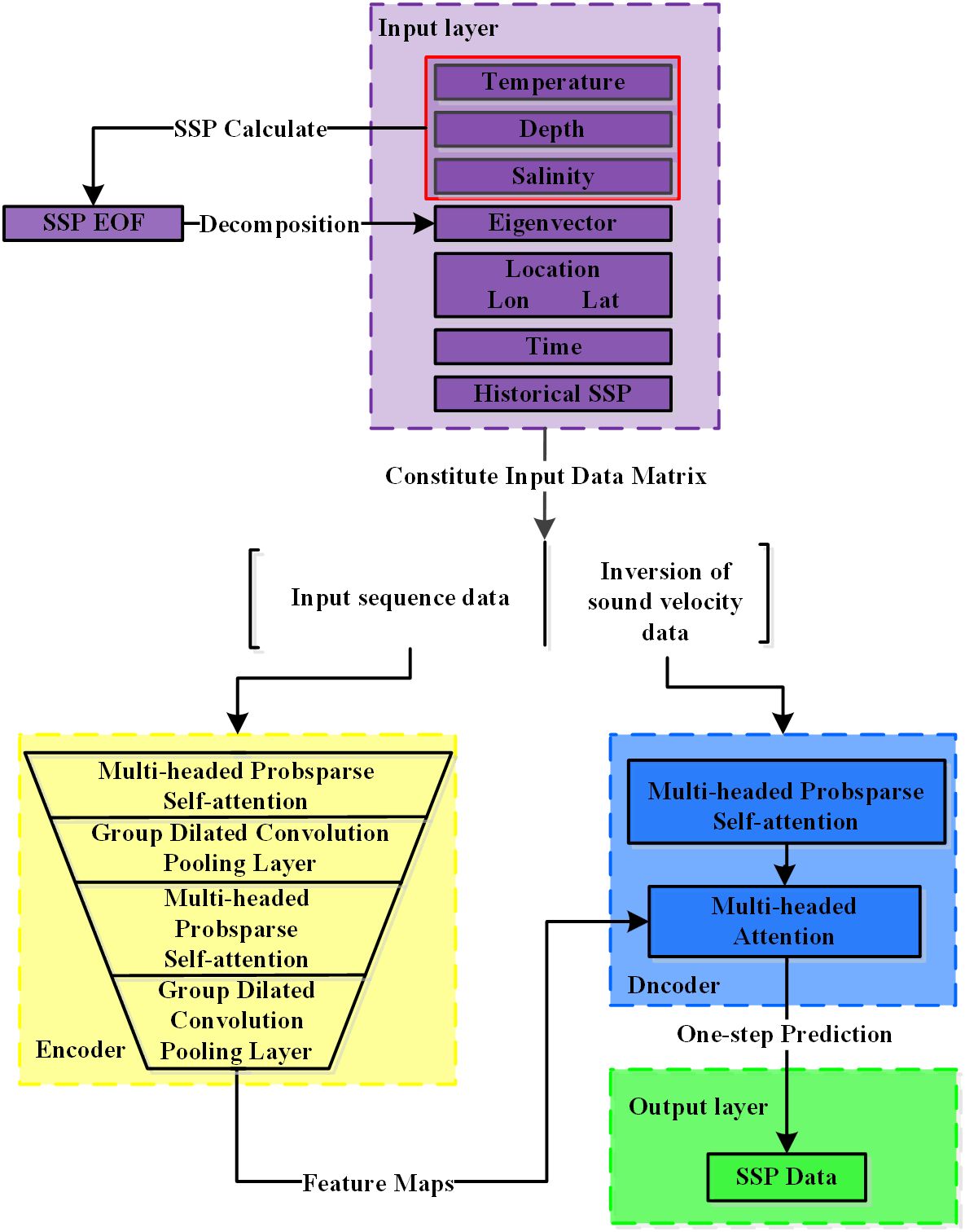
Figure 2. SSP Inversion Workflow with the Informer-GDC Model.

Step 1: Temperature, depth, and salinity data from a specific regional dataset are extracted and employed alongside an empirical formula to produce the corresponding SSP. Subsequently, SSP should be decomposed using EOF, with the resulting components incorporated as part of the input dataset.

Step 2: The temperature data, depth data, salinity data, features derived from EOF decomposition, geographical information (including latitude and longitude), temporal data, and historical SSP data must be integrated into a comprehensive input data matrix. This matrix is subsequently partitioned into two sections. Following this, the input sequence data is inverted to produce the sound velocity data.

Step 3: The input sequence data is subsequently processed by the encoder layer. Within this layer, the Multi-headed ProbSparse Self-attention module effectively filters the features of the input data. Additionally, the group dilated convolution, in conjunction with pooling layers, produces feature maps that are utilized by the Multi-headed self-attention mechanism in the decoder layer.

Step 4: The inverted sound velocity data is subsequently processed by the multi-headed ProbSparse self-attention module, after which it is further input into the multi-headed self-attention module.

Step 5: A one-step prediction is conducted to generate SSP data for the specified location.

3 Data and evaluation metrics

3.1 Argo data

Hangzhou Global Ocean Argo Scientific Observation Research Station (Li et al., 2017) provides global ocean temperature and salinity profile data with a spatial resolution of 1°×1°. The dataset includes different types of data files, such as annual averages, monthly averages, and monthly data files over several years. The vertical resolution spans 58 layers within the 0-2000 dbar range.Argo gridded dataset, covering the period from January 2008 to December 2018, was utilized as the experimental dataset (ftp://ftp.argo.org.cn/pub/ARGO/global/). The dataset from January 2008 to December 2017 served as the training dataset, while the dataset from 2018 was designated as the test dataset. SSP was calculated in accordance with the Mackenzie formula (Mackenzie, 1981). The Mackenzie formula is another commonly used empirical equation for sound speed calculation, applicable under general oceanic conditions, particularly when temperature and salinity variations are minimal (Mackenzie, 1966). The formula is expressed as follows:

$\begin{array}{ll}\begin{array}{c}C=1420.4+5.04T-0.056T^2+0.00029T^3\hfill \\ +(1.34+0.016T)(S-35)+0.016P\hfill \end{array}& (8)\end{array}$

Where C is the sound speed (m/s); T is the temperature (°C); S is the salinity (ppt); P is the pressure (dbar).

Four experimental regions were selected (Figure 3A). Region 1 corresponds to Bay of Bengal (84°-90°E, 10°-16°N), Region 2 pertains to South China Sea (113°-118°E, 8°-14°N), Region 3 encompasses Pacific Ocean (132°-138°E, 23°-29°N), and Region 4 is also located in Pacific Ocean (157°-163°E, 33°-39°N). The red boxes labeled a, b, c, and d indicate the locations of SSP inversion as determined by the model, specifically at coordinates 85°E, 15°N; 115°E, 12°N; 135°E, 25°N; and 160°E, 35°N, respectively. Figures 3B, C illustrates the annual mean temperature and salinity distributions across the longitudinal range of 85°E to 180°E and the latitudinal range of 0°N to 50°N.

Figure 3

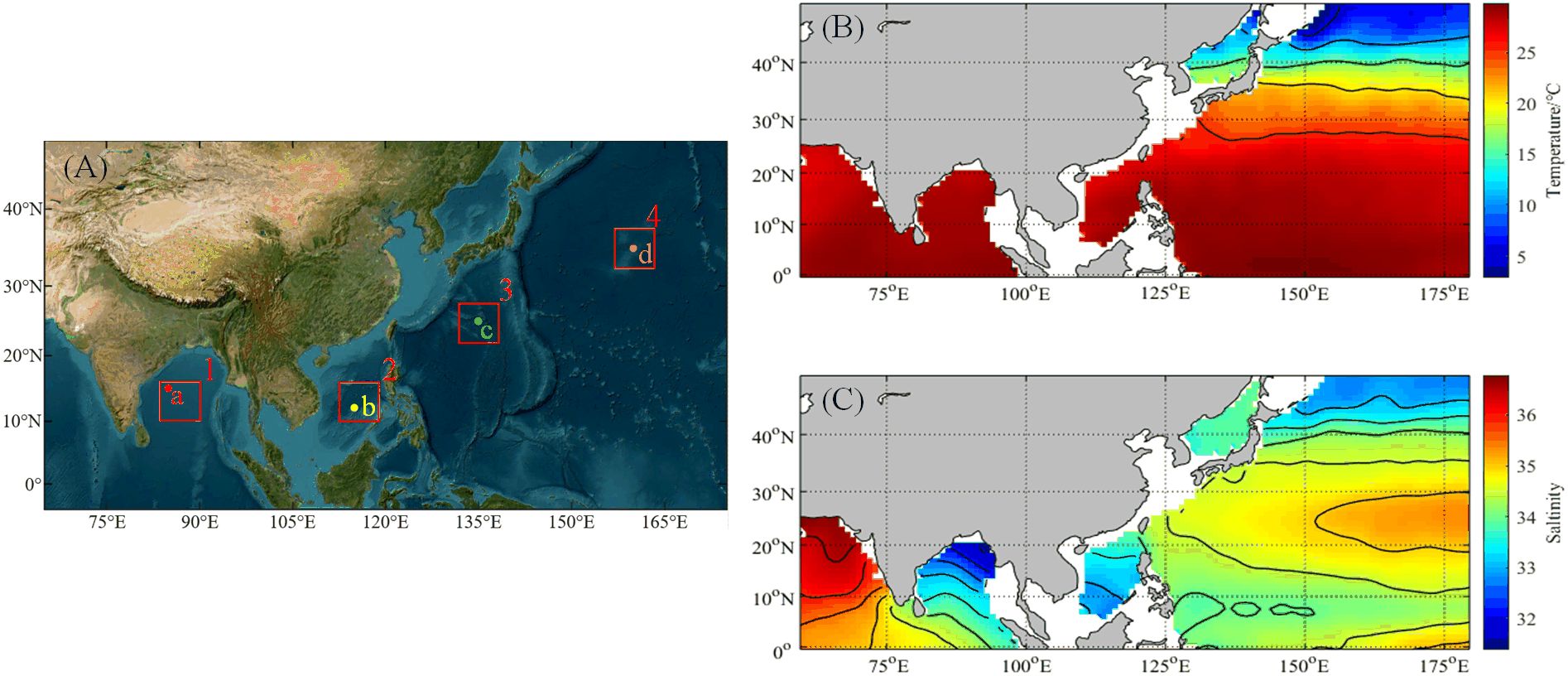
Figure 3. Distribution of experimental area locations.

3.2 EOF analysis

The historical SSP data from the training sample datasets across the four experimental regions were analyzed using EOF decomposition. The first five modes resulting from this analysis are depicted in Figure 3. The characteristic values of the first through fifth modes are predominantly concentrated within the depth range of 0 m to -800 m, with variations below -800 m approaching negligible levels. Figure 4A illustrates that sound speed perturbations are primarily concentrated between 0 m and -600 m, while (Figure 4B) indicates a concentration between 0 m and -1000 m. Figure 4C demonstrates that these perturbations are concentrated between 0 m and -1200 m, and (Figure 4D) further indicates a concentration between 0 m and -800 m. Table 1 presents the contribution rates of the first five eigenvectors derived from the EOF decomposition at various locations, revealing that the cumulative contribution rate of these five modes exceeds 95%. These initial five modal components are integrated into the training sample data.

Figure 4

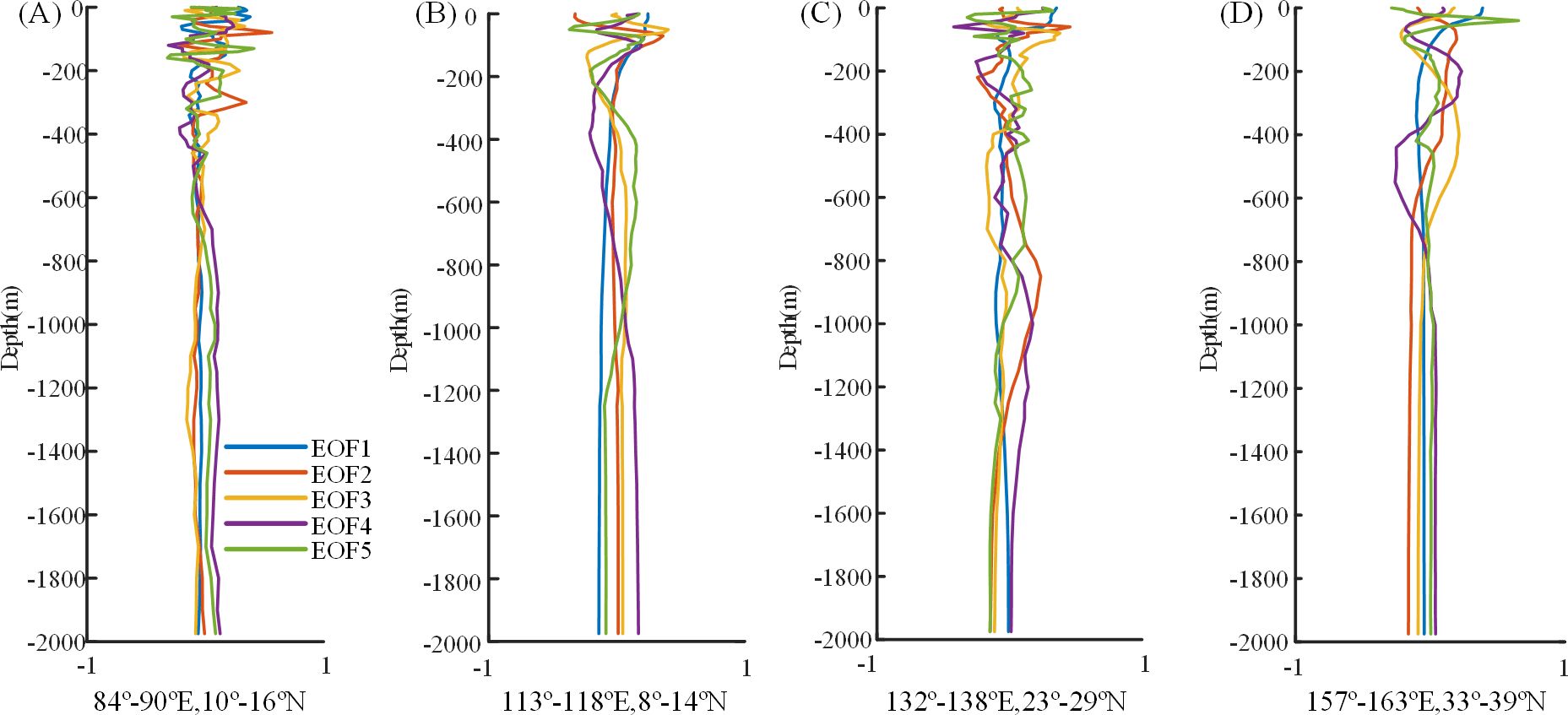
Figure 4. EOF modal features at each location.

Table 1

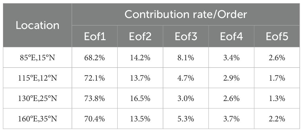
Table 1. Feature contribution rate and order.

3.3 Evaluation metrics

To assess the accuracy of the model’s inversion of SSP, three primary metrics have been established: mean absolute error (MAE), root mean square error (RMSE), and mean absolute percentage error (MAPE). These evaluation criteria have been specifically designed for sound speed inversion (Liu and Li, 2021; Liu and Qu, 2023; Qu et al., 2024). The corresponding equations are expressed as follows:

$\begin{array}{ll}\begin{array}{c}\mathit{M}\mathit{A}\mathit{E}\mathbf{=}\frac{{\mathbf{\sum }}_{\mathit{i}\mathbf{=}\mathbf{1}}^{\mathit{n}}\mathbf{|}{\mathit{y}}_{\mathit{t}\mathit{r}\mathit{u}\mathit{e}}\mathbf{-}{\mathit{y}}_{\mathit{i}\mathit{n}\mathit{v}\mathit{e}\mathit{r}}\mathbf{|}}{\mathit{n}}\end{array}& (9)\end{array}$

$\begin{array}{ll}\begin{array}{c}\mathit{M}\mathit{S}\mathit{E}\mathbf{=}\sqrt{\frac{{\mathbf{\sum }}_{\mathit{i}\mathbf{=}\mathbf{1}}^{\mathit{n}}{({\mathit{y}}_{\mathit{t}\mathit{r}\mathit{u}\mathit{e}}\mathbf{-}{\mathit{y}}_{\mathit{i}\mathit{n}\mathit{v}\mathit{e}\mathit{r}})}^{\mathbf{2}}}{\mathit{n}}}\end{array}& (10)\end{array}$

$\begin{array}{ll}\begin{array}{c}\mathit{M}\mathit{A}\mathit{P}\mathit{E}\mathbf{=}\frac{{\mathbf{\sum }}_{\mathit{i}\mathbf{=}\mathbf{1}}^{\mathit{n}}\left(\frac{\mathbf{|}{\mathit{y}}_{\mathit{t}\mathit{r}\mathit{u}\mathit{e}}\mathbf{-}{\mathit{y}}_{\mathit{i}\mathit{n}\mathit{v}\mathit{e}\mathit{r}}\mathbf{|}}{{\mathit{y}}_{\mathit{t}\mathit{r}\mathit{u}\mathit{e}}}\right)}{\mathit{n}}\mathbf{\times }\mathbf{100}\mathbf{\%}\end{array}& (11)\end{array}$

where ${\mathit{y}}_{\mathit{t}\mathit{r}\mathit{u}\mathit{e}}$ represents the measured value of SSP; ${\mathit{y}}_{\mathit{i}\mathit{n}\mathit{v}\mathit{e}\mathit{r}}$ represents the inverted value of the SSP; and n represents the number of data samples.

4 Results and discussion

In accordance with the calculation formula for SSP, the magnitude of SSP is influenced by both temperature and salinity. However, various factors can impact the temperature and salinity of seawater (Zhang et al., 2017). To ensure an accurate inversion of SSP at a specific location, it is crucial to consider several additional factors, including the geographical location of the inversion, temporal variations, oceanic activity, and the marine environment. This study involved two experiments designed to demonstrate the effectiveness and accuracy of Informer-GDC model in performing inversions. Subsequently, the performance of Informer-GDC model was compared with that of LSTM and Informer models to establish the superiority of the proposed model.

4.1 SSP inversion across different depths

To assess the accuracy of SSP inversion executed by Informer-GDC model, Region 2 was designated as the experimental site, and SSP inversion was performed at Location b(115°E, 12°N). SSP inversion results generated by the proposed model were subsequently compared with the actual SSP data collected in March (Figure 5).

Figure 5

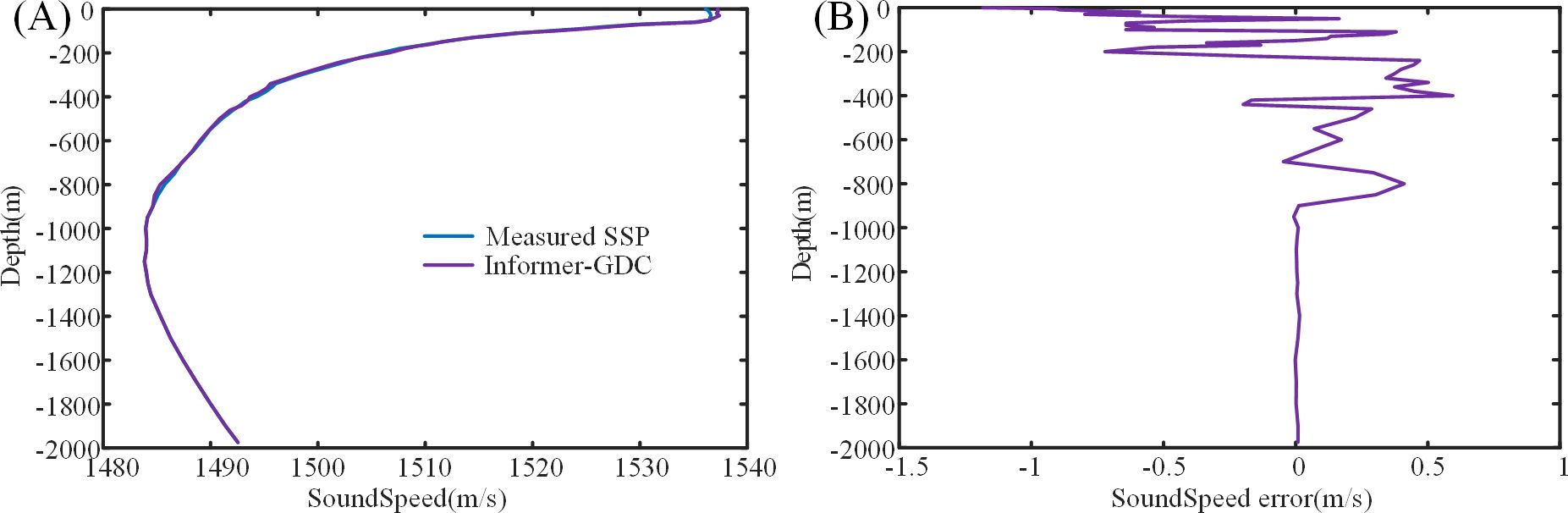
Figure 5. SSP inversion using the Informer-GDC Model.

In Figure 5, SSP inverted by Informer-GDC model exhibits a strong correlation with the measured SSP, with only minimal discrepancies in the values. The analysis of the inversion sound speed error data in Table 2 indicates that the most significant sound speed error in the model inversion occurs within the depth range of 0 m to 200 m, characterized by mean squared error (MSE) of 0.575 m/s, MAE of 0.527 m/s, and MAPE of 0.034%. The temperature at the inversion site displays marked seasonal variations, with the lowest temperatures recorded during the winter months, exhibiting minimal fluctuations. In contrast, a significant increase in the daily average temperature is observed in March. The temperature and salinity of the surface layer are notably affected by monsoons, solar radiation, and disturbances in seawater, leading to more pronounced variations. Additionally, the salinity at this location is influenced by seawater intrusion from the Luzon Strait and Mindoro Strait, resulting in a sustained increase in salinity levels (Zhang et al., 2016; Yi et al., 2020; Yang et al., 2023). However, during this period, the effect of rainfall on surface layer salinity is minimal, complicating the changes in seawater salinity. As depth increases, the influence of seawater salinity and temperature on sound speed inversion diminishes, leading to a reduction in all error metrics. Within the depth range of 0 m to 2000 m, the overall sound speed inversion errors of the model are as follows: MSE of 0.387 m/s, MAE of 0.527 m/s, and MAPE of 0.019%. The consistently low error rates in sound speed inversion indicate that the model is proficient in accurately inverting SSP.

Table 2

Table 2. Evaluation Metrics of Sound Speed Profiles Inverted by Informer-GDC at Different Depths.

4.2 SSP inversion across different times

Region 3 was designated as the experimental area, and SSP at Location C was inverted. The temperature and salinity at this location exhibit considerable seasonal variations across different time periods, which poses a challenge to the accuracy and stability of the model’s inversion. Figure 6 presents a comparison of SSP inversions generated by Informer-GDC model across four seasons alongside the measured SSP, indicating that the inversion errors in sound velocity predominantly fall within the range of 0 m to 400 m. Table 3 demonstrates that, although the inversion metrics of the model are relatively consistent in March and December, the sound velocity error is most pronounced in September, followed by June.

Figure 6

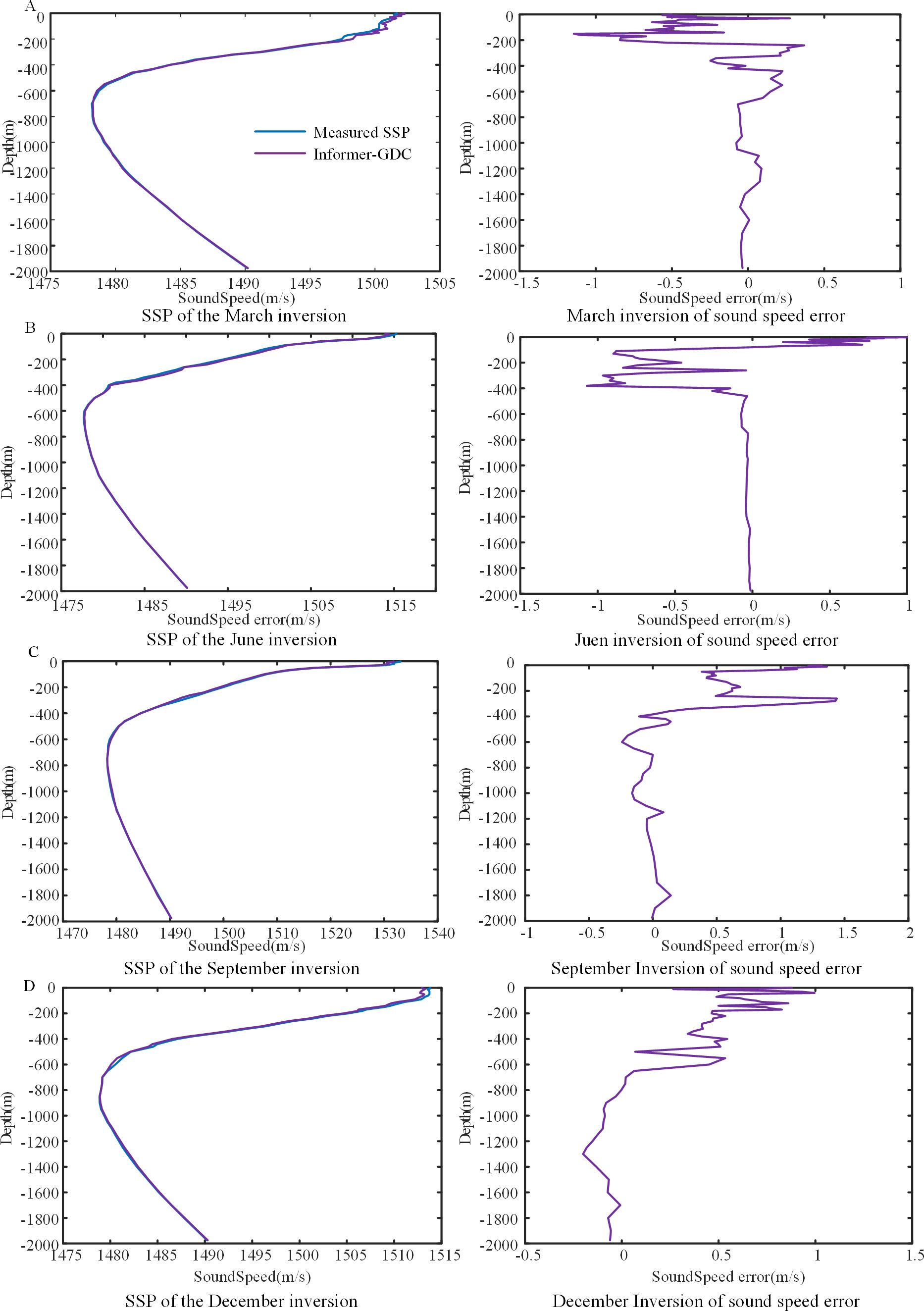
Figure 6. SSP inversion for different months.

Table 3

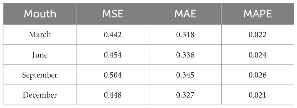
Table 3. Evaluation Metrics of Sound Velocity Profiles Inverted by Informer-GDC in Different Months.

In particular, the inversion error metrics for September are shown as follows: MSE = 0.504 m/s, MAE = 0.345 m/s, and MAPE = 0.022%. When compared to the results obtained in September, the metrics for the other two months (March and December) exhibit average reductions of 10.91%, 5.56%, and 16.7% for MSE, MAE, and MAPE, respectively. In both March and December, the concentration of sound velocity errors is observed at depths ranging from 0 m to 450 m, with a notable increase in the magnitude of errors occurring closer to the ocean surface. The maximum recorded errors were -1.344 m/s and 0.878 m/s, respectively. The larger errors in the surface layer may be attributed to the inversion location being situated within the highly dynamic Kuroshio Current region (Hsin et al., 2006), where intense oceanic mixing leads to significant alterations in surface salinity. While temperature fluctuations in March and December are relatively minor, the substantial variations in salinity result in more pronounced inversion errors. In June, sound velocity errors are concentrated between depths of 0 m and 820 m. During this period, solar radiation heats the seawater more uniformly. However, seasonal rainfall introduces a considerable volume of freshwater, leading to more significant changes in seawater temperature and salinity (Hackert and Ballabrera-Poy, 2011). Additionally, the region is affected by vortex transport. In September, the larger sound velocity errors are influenced not only by the aforementioned factors but also by seasonal rainfall, monsoons, and diurnal variations, which contribute to more pronounced changes in sound velocity. The results of Informer-GDC model across different months demonstrate consistent evaluation metrics, indicating that the model exhibits a high degree of accuracy.

4.3 Sound velocity profiles inverted across different models and locations

To demonstrate the superiority of the proposed model for inverting SSP, a comparative analysis was performed involving SSP inverted by LSTM model, Informer model, and Informer-GDC model, alongside the corresponding measured SSP. The experimental datasets were selected from Regions 1 and 4, with validation conducted at Locations A and D within these regions, as shown in Figures 7 and 8. To maintain the integrity of the experimental design, all inversion models were trained on the same dataset and employed identical parameters. The specific configurations for the model parameters are outlined in Table 4.

Figure 7

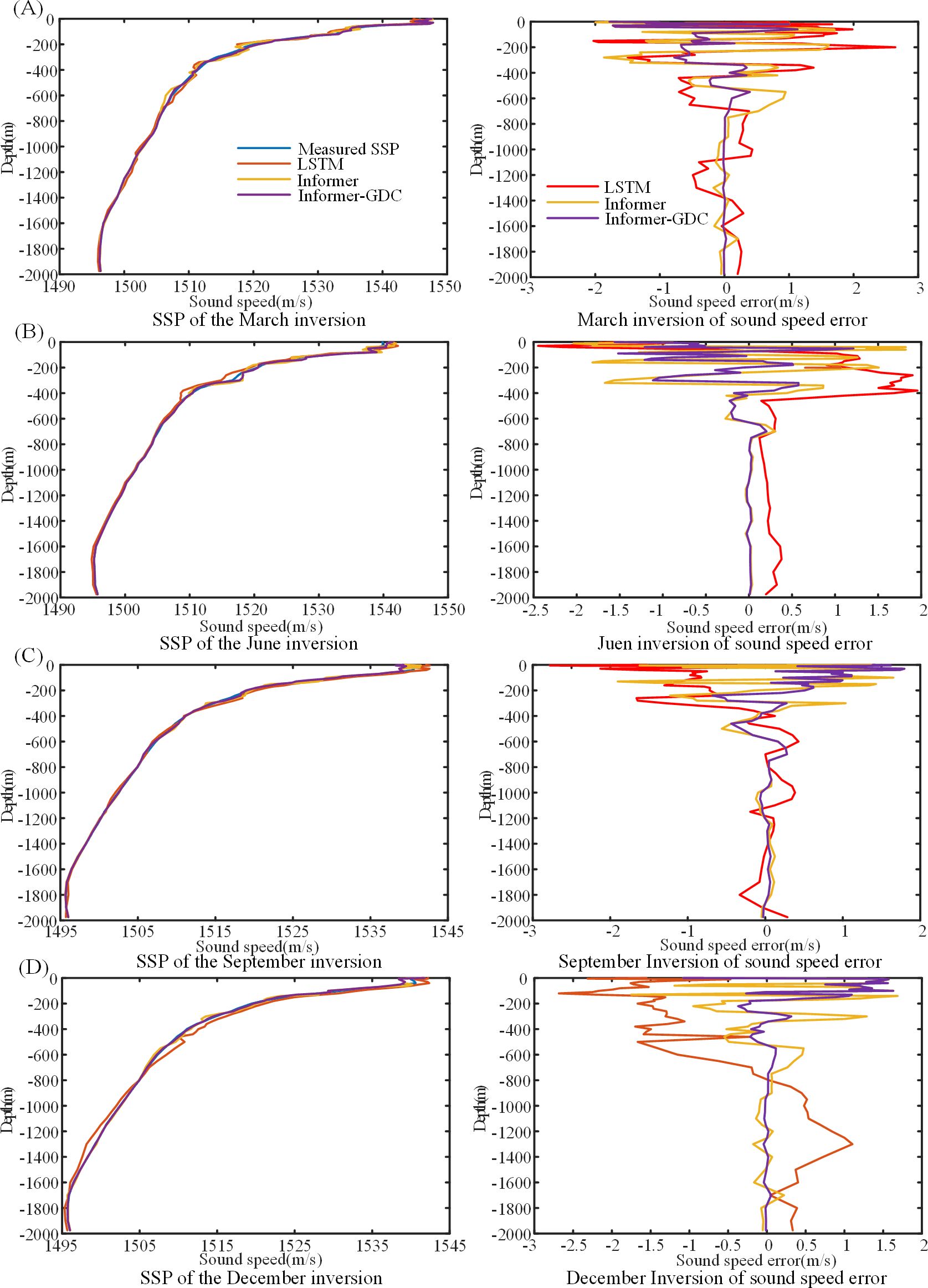
Figure 7. SSP Inversion by different models (Region 1).

Figure 8

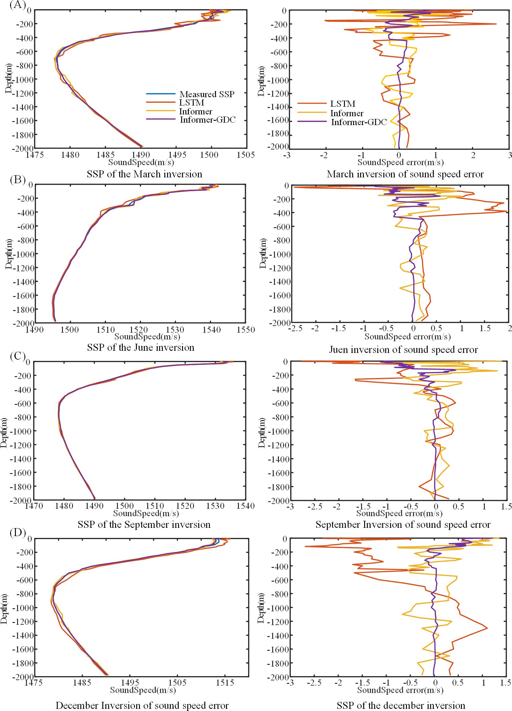
Figure 8. SSP Inversion by different models (Region 4).

Table 4

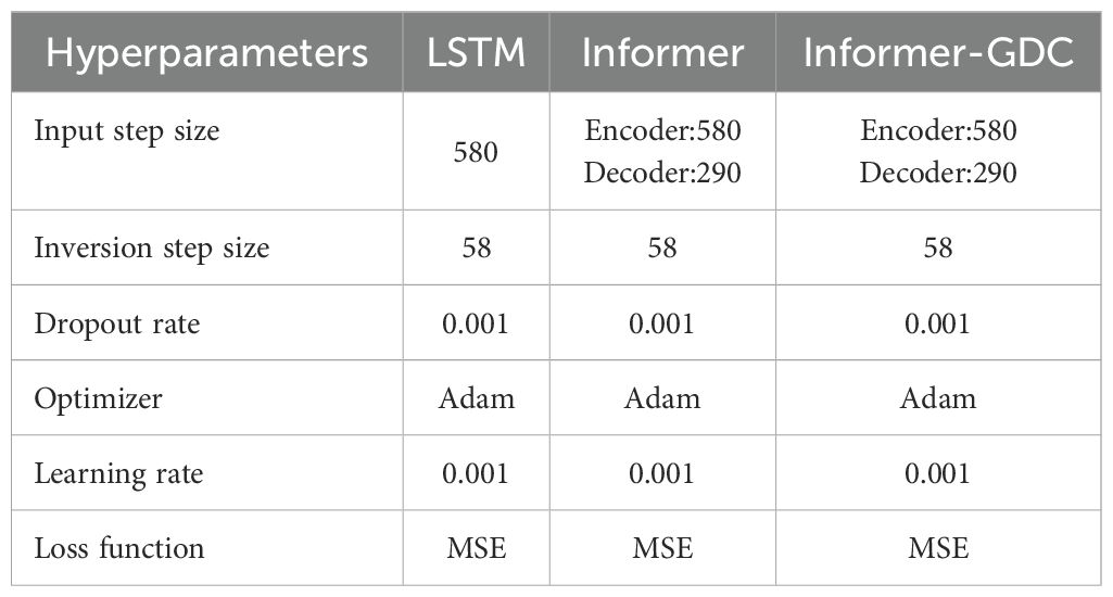
Table 4. Model parameter settings.

SSP inversion in Region 1 is located in proximity to the equator, where it experiences a relatively stable annual temperature range of 24°C to 30°C. The temperature profile exhibits a bimodal structure, characterized by minor fluctuations from June to November. Notably, in September, a significant diurnal temperature variation is observed, leading to considerable shifts in the surface layer temperature. Seasonal variations in salinity are pronounced and are primarily influenced by the equatorial current system, monsoons, and precipitation patterns (Gao et al., 2024). For instance, during the summer and autumn months, substantial runoff occurs from Brahmaputra and Ganges rivers, with the region’s average annual precipitation ranging from 1,000 mm to 3,000 mm. This influx of freshwater results in a dilution of seawater salinity, while the effects of the monsoon facilitate significant exchanges between seawater and the Indian Ocean, leading to notable changes in salinity.

The variability of seawater in Region 4 demonstrates similarities to that observed in Region 3. Therefore, it will not be examined in further detail. It is noteworthy that the seasonal variations in Region 4 exert a more significant influence compared to those in Region 3. Consequently, the inversion of sound velocity in the surface layer becomes a more complex process, imposing greater demands on the inversion model.

Tables 5, 6 demonstrate that Informer-GDC model exhibits superior accuracy in comparison to the other two models for SSP inversion at both locations. At Location A, all three models achieve high accuracy in SSP inversion. Specifically, the sound velocity error metrics for LSTM model over the four-month period are as follows: MSE = 1.102 m/s, MAE = 0.908 m/s, and MAPE = 0.058%. SSP inversion errors associated with Informer model show improvements of 51.23%, 52.18%, and 49.57% across the three evaluation standards when compared to LSTM model. Furthermore, Informer-GDC model enhances these metrics by 31.76%, 43.08%, and 36.18% relative to Informer model. At Location D, the accuracy of sound velocity inversion achieved by Informer-GDC model reflects improvements of 29.56%, 37.48%, and 37.98% when compared to Informer model, and 41.78%, 52.12%, and 52.85% when compared to LSTM model. The results of the experimental analysis conducted across four seasons at both locations indicate that SSP inversion utilizing the proposed Informer-GDC model is more closely aligned with the measured SSP values, thereby substantiating the superiority of the proposed method.

Table 5

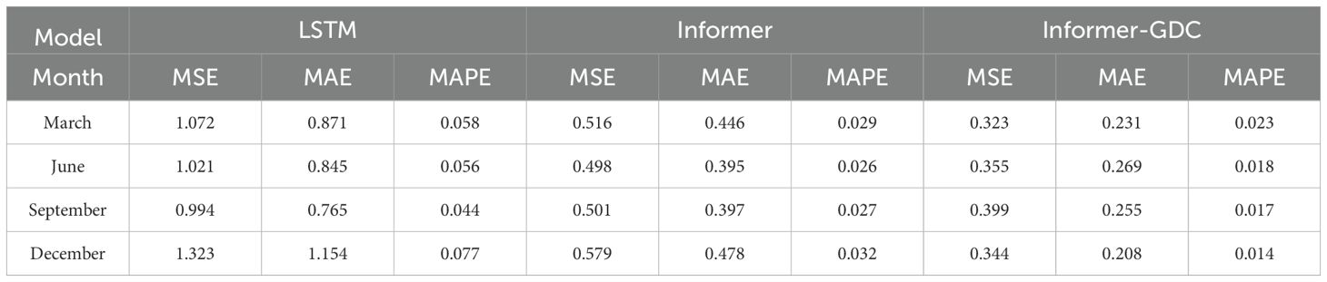
Table 5. Comparison of sound velocity profile errors inverted by different modes.

Table 6

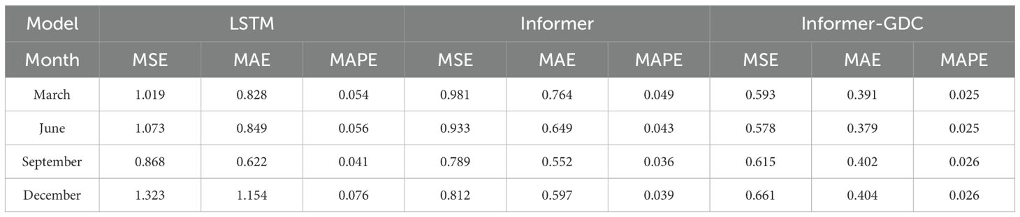
Table 6. Comparison of sound velocity profile errors inverted by different modes.

5 Conclusion

The complexity and dynamics of the oceanic environment lead to significant variations in SSP, particularly within the surface layer. Accurate and rapid acquisition of SSP data is crucial for marine research and engineering. While traditional machine learning approaches to SSP inversion have demonstrated sufficient accuracy for research purposes, the demand for higher precision SSP inversion is particularly relevant to the field of ocean engineering.

This study proposes a novel GDC optimization within the Informer model for SSP inversion. The model was trained using a comprehensive dataset from the Argo project, which included temperature, salinity, depth, EOF-decomposed eigenvectors, latitude, longitude, time, and historical SSP data from 2008 to 2017. The Informer-GDC model was validated through preliminary experiments conducted in the South China Sea, where it demonstrated high accuracy with an MSE of 0.387 m/s, MAE of 0.527 m/s, and MAPE of 0.019%. Additional validation using data from different months in the Pacific Ocean confirmed the model’s robustness, with an average MSE of 0.48 m/s, MAE of 0.31 m/s, and MAPE of 0.02%.

A comparative analysis was conducted to evaluate the inversion performance of the Informer-GDC model against the LSTM model and the standard Informer model across different regions and time periods. The results indicate that the Informer-GDC model significantly outperforms both models in SSP inversion accuracy. Specifically, the Informer-GDC model improved the MSE, MAE, and MAPE by an average of 46.51%, 29.66%, and 51.65%, respectively, compared to the LSTM model, and by 39.28% and 51.25% compared to the standard Informer model. These findings validate the Informer-GDC model as a robust and superior approach for SSP inversion.

Looking forward, future research will focus on incorporating additional factors that influence sound speed, such as meteorological conditions, monsoon patterns, and ocean currents. Integrating these variables is expected to enhance the model’s precision and applicability, ultimately contributing to advancements in oceanographic research while reducing associated costs and workloads.

Data availability statement

The original contributions presented in the study are included in the article/supplementary material. Further inquiries can be directed to the corresponding author.

Author contributions

SQ: Data curation, Investigation, Methodology, Project administration, Resources, Software, Validation, Writing – original draft, Writing – review & editing, Formal analysis. YZ: Data curation, Formal analysis, Investigation, Methodology, Project administration, Supervision, Validation, Writing – review & editing. ZC: Data curation, Funding acquisition, Investigation, Methodology, Resources, Supervision, Validation, Writing – review & editing, Formal analysis, Project administration.

Funding

The author(s) declare that no financial support was received for the research, authorship, and/or publication of this article.

Conflict of interest

The authors declare that the research was conducted in the absence of any commercial or financial relationships that could be construed as a potential conflict of interest.

Publisher’s note

All claims expressed in this article are solely those of the authors and do not necessarily represent those of their affiliated organizations, or those of the publisher, the editors and the reviewers. Any product that may be evaluated in this article, or claim that may be made by its manufacturer, is not guaranteed or endorsed by the publisher.

References

Ballard M. S., Frisk G. V., Becker K. M. (2014). Estimates of the temporal and spatial variability of ocean sound speed on the New Jersey shelf. J. Acoustical Soc. America 135, 3316–3326. doi: 10.1121/1.4875715

PubMed Abstract | Crossref Full Text | Google Scholar

Bianco M., Gerstoft P. (2017). Dictionary learning of sound speed profiles. J. Acoustical Soc. America 141, 1749–1758. doi: 10.1121/1.4977926

PubMed Abstract | Crossref Full Text | Google Scholar

Bianco M. J., Gerstoft P., Traer J., Ozanich E., Roch M. A., Gannot S., et al. (2019). Machine learning in acoustics: Theory and applications. J. Acoustical Soc. America 146, 3590–3628. doi: 10.1121/1.5133944

PubMed Abstract | Crossref Full Text | Google Scholar

Castro-Correa J., Arnett S., Neilsen T., Wan L., Badiey M. (2022). Supervised classification of sound speed profiles via dictionary learning. J. Atmospheric Oceanic Technol. 40, 99–112. doi: 10.1175/jtech-d-21-0090.1

Crossref Full Text | Google Scholar

Chen L.-C., Papandreou G., Kokkinos I., Murphy K., Yuille A. L. (2018). DeepLab: semantic image segmentation with deep convolutional nets, atrous convolution, and fully connected CRFs. IEEE Trans. Pattern Anal. Mach. Intell. 40, 834–848. doi: 10.1109/tpami.2017.2699184

PubMed Abstract | Crossref Full Text | Google Scholar

Chen T., Duan B., Sun Q., Zhang M., Li G., Geng H., et al. (2022). An efficient sharing grouped convolution via bayesian learning. IEEE Trans. Neural Networks Learn. Syst. 33, 7367–7379. doi: 10.1109/tnnls.2021.3084900

PubMed Abstract | Crossref Full Text | Google Scholar

Davis R. E. (1976). Predictability of sea surface temperature and sea level pressure anomalies over the north pacific ocean. J. Phys. Oceanography 6, 249–266. doi: 10.1175/1520-0485(1976)006<0249:possta>2.0.co;2

Crossref Full Text | Google Scholar

DeSanto J. (1984). Oceanic sound speed profile inversion. IEEE J. Oceanic Eng. 9, 12–17. doi: 10.1109/joe.1984.1145593

Crossref Full Text | Google Scholar

Feng X., Tian T., Zhou M., Sun H., Li D., Tian F., et al. (2024). Sound speed inversion based on multi-source ocean remote sensing observations and machine learning. Remote Sens. 16, 814. doi: 10.3390/rs16050814

Crossref Full Text | Google Scholar

Feng Y., Zhang T., Sah A. P., Han L., Zhang Z. (2021). Using appearance to predict pedestrian trajectories through disparity-guided attention and convolutional LSTM, in IEEE transactions on vehicular technology. 70 (8), 7480–7494. doi: 10.1109/TVT.2021.3094678

Crossref Full Text | Google Scholar

Gao G., Yao B., Li Z., Duan D., Zhang X. (2024). Forecasting of sea surface temperature in eastern tropical pacific by a hybrid multiscale spatial–temporal model combining error correction map. IEEE Trans. Geosci. Remote Sens. 62, 1–22, 4204722. doi: 10.1109/TGRS.2024.3353288

Crossref Full Text | Google Scholar

Hackert E., Ballabrera-Poy J. (2011). Impact of sea surface salinity assimilation on coupled forecasts in the tropical Pacific. J. Geophys Res: Oceans. 116, C05027. doi: 10.129/2010JC006708

Crossref Full Text | Google Scholar

Heidemann J., Stojanovic M., Zorzi M. (2012). Underwater sensor networks: applications, advances and challenges. Philos. Trans. R. Soc. A: Mathematical Phys. Eng. Sci. 370, pp.158–pp.175. doi: 10.1098/rsta.2011.0214

PubMed Abstract | Crossref Full Text | Google Scholar

Hou H., Xu Y., Chen M., Zhi L., Guo W., Gao M., et al. (2020). Hierarchical long short-term memory network for cyberattack detection. IEEE Access 8, pp.90907–90913. doi: 10.1109/access.2020.2983953

Crossref Full Text | Google Scholar

Huang W., Zhou J., Gao F., Wang J., Xu T. (2024). Experimental results of underwater sound speed profile inversion by few-shot multi-task learning. Remote Sens. 16 (1), 167. doi: 10.3390/rs16010167

Crossref Full Text | Google Scholar

Hsin Y. C., Wu C. R., Chao S. Y. (2006). Atmospheric sounding over the winter Kuroshio Extension: Effect of surface stability on atmospheric boundary layer structure. Geophys Res. Lett. 33, L12803. doi: 10.1029/2005GL025102

Crossref Full Text | Google Scholar

Huang Wu., Li D., Jiang P. (2018). “Underwater sound speed inversion by joint artificial neural network and ray theory,” in Proceedings of the 13th International Conference on Underwater Networks & Systems. (New York: ACM), 1–8. doi: 10.1145/3291940.3291972

Crossref Full Text | Google Scholar

Huang C., Wu M., Huang X. (2020). Reconstruction and evaluation of the full-depth sound speed profile with world ocean atlas 2018 for the hydrographic surveying in the deep sea waters. Appl. Ocean Res. 101, 102201–102201. doi: 10.1016/j.apor.2020.102201

Crossref Full Text | Google Scholar

Huang C.-F., Yang S.-F., Liu J.-Y. (2012). Inverting sediment sound speed profile using A parameterized geoacoustic model: numerical and statistical analysis. J. Mar. Sci. Technol. 20, 584–594. doi: 10.6119/jmst-012-0712-1

Crossref Full Text | Google Scholar

Jain S., Ali M. M. (2006). Estimation of sound speed profiles using artificial neural networks. IEEE Geosci. Remote Sens. Lett. 3, 467–470. doi: 10.1109/LGRS.2006.876221

Crossref Full Text | Google Scholar

Jeon Y., Kim J. (2021). Integrating multiple receptive fields through grouped active convolution. IEEE Trans. Pattern Anal. Mach. Intell. 43, 3892–3903. doi: 10.1109/tpami.2020.2995864

PubMed Abstract | Crossref Full Text | Google Scholar

Jiang G., He H., Yan J., Xie P. (2019). Multiscale convolutional neural networks for fault diagnosis of wind turbine gearbox. IEEE Trans. Ind. Electron. 66, 3196–3207. doi: 10.1109/tie.2018.2844805

Crossref Full Text | Google Scholar

LeBlanc L. R., Middleton F. H. (1980). An underwater acoustic sound velocity data model. J. Acoustical Soc. Am. 67 (6), 2055–2062. doi: 10.1121/1.384448

Crossref Full Text | Google Scholar

Leroy C. C., Robinson S. P., Goldsmith M. J. (2008). A new equation for the accurate calculation of sound speed in all oceans. J. Acoustical Soc. America 124, 2774–2782. doi: 10.1121/1.2988296

PubMed Abstract | Crossref Full Text | Google Scholar

Li H., Qu K., Zhou J. (2021). Reconstructing sound speed profile from remote sensing data: nonlinear inversion based on self-organizing map. IEEE Access 9, pp.109754–109762. doi: 10.1109/access.2021.3102608

Crossref Full Text | Google Scholar

Li J., Shi Y., Yang Y., Chen C. (2022). Comprehensive study of inversion methods for sound speed profiles in the south China sea. J. Ocean Univ. China 21, 1487–1494. doi: 10.1007/s11802-022-5001-7

Crossref Full Text | Google Scholar

Li H., Xu F., Zhou W., Wang D., Wright J. S., Liu Z., et al. (2017). Development of a global gridded Argo data set with Barnes successive corrections. J. Geophysical Research: Oceans 122, 866–889. doi: 10.1002/2016jc012285

Crossref Full Text | Google Scholar

Lin G., Wu Q., Qiu L., Huang X. (2018). Image super-resolution using a dilated convolutional neural network. Neurocomputing 275, 1219–1230. doi: 10.1016/j.neucom.2017.09.062

Crossref Full Text | Google Scholar

Liu B., Jiayu L. (2010). Hydroacoustics principle. 2th (Harbin: Harbin Engineering University Press).

Google Scholar

Liu R., Li Z. (2021). The effects of bubble scattering on sound propagation in shallow water. J. Mar. Sci. Eng. 9, 1441. doi: 10.3390/jmse9121441

Crossref Full Text | Google Scholar

Liu C., Qu K. (2023). Wide-area sound speed profile estimation based on a pre-classification scheme for sound speed perturbation modes. Front. Mar. Sci. 10. doi: 10.3389/fmars.2023.1130061

Crossref Full Text | Google Scholar

Mackenzie K. V. (1966). Precision in-situ measurements of relationship between temperature, salinity, pressure, and sound speed. J. Acoust. Soc Am. 40, 1244–1245. doi: 10.1121/1.1943000

Crossref Full Text | Google Scholar

Mackenzie K. V. (1981). Nine-term equation for sound speed in the oceans. J. Acoustical Soc. America 70, 807–812. doi: 10.1121/1.386920

Crossref Full Text | Google Scholar

Piao S., Yan X., Li Q., Li Z., Wang Z., Zhu J. (2023). Time series prediction of shallow water sound speed profile in the presence of internal solitary wave trains. Ocean Eng. 283, 115058. doi: 10.1016/j.oceaneng.2023.115058

Crossref Full Text | Google Scholar

Qu K., Yin W., Zhu F., Meng L. (2024). Modeling sound speed profile based on ocean normal mode. Front. Mar. Sci. 11. doi: 10.3389/fmars.2024.1378396

Crossref Full Text | Google Scholar

Smith T. M., Reynolds R. W., Livezey R. E., Stokes D. C. (1996). Reconstruction of historical sea surface temperatures using empirical orthogonal functions. J. Climate 9, 1403–1420. doi: 10.1175/1520-0442(1996)009%3C1403:rohsst%3E2.0.co;2

Crossref Full Text | Google Scholar

Talib K. H., Othman M. Y., Wazir M. A. M., Azizan A. (2011). “Determination of speed of sound using empirical equations and SVP,” in 2011 IEEE 7th International Colloquium on Signal Processing and its Applications. (Kuala Lumpur: IEEE), 1–4. doi: 10.1109/cspa.2011.5759882

Crossref Full Text | Google Scholar

Tong G., Ge Z., Peng D. (2024). RSMformer: an efficient multiscale transformer-based framework for long sequence time-series forecasting. Appl. Intell. 54, 1275–1296. doi: 10.1007/s10489-023-05250-8

Crossref Full Text | Google Scholar

Wang F., Liu R., Hu Q., Chen X. (2021). Cascade convolutional neural network with progressive optimization for motor fault diagnosis under nonstationary conditions. IEEE Trans. Ind. Inf. 17, 2511–2521. doi: 10.1109/tii.2020.3003353

Crossref Full Text | Google Scholar

Wang J., Xu T., Nie W., Yu X. (2020). The construction of sound speed field based on back propagation neural network in the global ocean. Mar. Geodesy 43 (6), 621–642. doi: 10.1080/01490419.2020.1815912

Crossref Full Text | Google Scholar

Xia H., Sun W., Song S., Mou X. (2020). Md-net: multi-scale dilated convolution network for CT images segmentation. Neural Process. Lett. 51, 2915–2927. doi: 10.1007/s11063-020-10230-x

Crossref Full Text | Google Scholar

Yang H., Lee K., Choo Y., Kim K. (2020). Underwater acoustic research trends with machine learning: ocean parameter inversion applications. J. Ocean Eng. Technol. 34, 371–376. doi: 10.26748/ksoe.2020.016

Crossref Full Text | Google Scholar

Yang Z., Liu L., Li N., Tian J. (2022). Time series forecasting of motor bearing vibration based on informer. Sensors 22, 5858. doi: 10.3390/s22155858

PubMed Abstract | Crossref Full Text | Google Scholar

Yang B., Ma T., Huang X. (2023). ATFSAD: enhancing long sequence time-series forecasting on air temperature prediction. IEEE Access 11, 92080–92091. doi: 10.1109/access.2023.3308693

Crossref Full Text | Google Scholar

Yi D. L., Melnichenko O., Hacker P., Potemra J. (2020). Remote sensing of sea surface salinity variability in the South China Sea. J. Geophys Res: Oceans. 125, e2020JC016827. doi: 10.1029/2020JC016827

Crossref Full Text | Google Scholar

Yuan H., Shuaidong J., Shaohua J., Lihua Z., Hua W. (2023). Correction for crowd sourced bathymetry data using GA-NN model to inverse sound velocity profiles. Geomatics Inf. Sci. Wuhan Univ. 48, 377–385. doi: 10.13203/j.whugis20200515

Crossref Full Text | Google Scholar

Zhang Q., Guo X., Ma L. (2017). The research of the characteristics of the ocean ambient noise under varying environment. J. Comput. Acoustics 25, 1750021–1750021. doi: 10.1142/s0218396x17500217

Crossref Full Text | Google Scholar

Zhang W. Z., Wang H., Chai F., Qiu G (2016). Physical drivers of chlorophyll variability in the open South China Sea. J. Geophys Res: Oceans. 121, 7123–7140. doi: 10.1002/2016JC011983

Crossref Full Text | Google Scholar

Zhou H., Zhang S., Peng J., Zhang S., Li J., Xiong H., et al. (2021). Informer: beyond efficient transformer for long sequence time-series forecasting. Proc. AAAI Conf. Artif. Intell. 35, 11106–11115. doi: 10.1609/aaai.v35i12.17325

Crossref Full Text | Google Scholar

Zhu W., Li H., Cheng X., Jiang Y. (2023). A multi-task road feature extraction network with grouped convolution and attention mechanisms. Sensors 23, 8182–8182. doi: 10.3390/s23198182

PubMed Abstract | Crossref Full Text | Google Scholar