Calculating 3D rugosity maps for complex habitat scans

Advances in 3D scanning and reconstruction techniques, such as structure-from-motion, have resulted in an abundance of increasingly-detailed 3D habitat models. However, many existing methods for calculating structural complexity of these models use 2.5D techniques that fail to capture the details of truly 3D models with overlapping features. This paper presents novel algorithms that extend traditional rugosity metrics to generate multi-scale rugosity maps for complex 3D models. Models are repeatedly subdivided for local analysis using multiple 3D grids, which are jittered to smooth results and suppress extreme values from edge cases and poorly-fit reference planes. A rugosity-minimizing technique is introduced to find optimal reference planes for the arbitrary sections of the model within each grid cell. These algorithms are implemented in an open-source analysis software package, HabiCAT 3D (Habitat Complexity Analysis Tool), that calculates and visualizes high-quality 3D rugosity maps for large and complex models. It also extends fractal dimension and vector dispersion complexity metrics, and is used in this paper to evaluate and discuss the appropriateness of each metric to various coral reef datasets.

1 Introduction

Habitat structural complexity is a critical feature shaping a range of ecosystem functions, including predator-prey interactions, food web structure and biodiversity (Smith et al., 2014). One of the more widely-used and supported measures of structural complexity is rugosity (R), the amount of surface area within the same planar area (Loke and Chisholm, 2022). Rugosity is frequently measured in kelp and terrestrial forests (Gough et al., 2022), intertidal reefs (Mazzuco et al., 2020), and coral reefs (Young et al., 2017; Pascoe et al., 2021). The traditional measurements of rugosity are those collected in-situ using the surface area (ratio of the actual surface area to that of a plane with the same dimensions) (Roberts and Ormond, 1987) and the chain-and-tape index (ratio of the apparent distance to the linear distance) (Stoner and Lewis, 1985; Warfe et al., 2008). With the advent of 3D modeling and mapping, digital rugosity measurements have gained a strong foothold in measuring complexity (Loke and Chisholm, 2022). With an accurate model, digital measurement accuracy surpasses that of the foundational, in-situ methods in rugosity measurements (Young et al., 2017; Bayley et al., 2019), as continuous measurements across the model more accurately reflect complexity of an area rather than just an estimation. Though complexity measurements from LiDAR generated models are finely detailed and accurate (Vierling et al., 2008), measurements from Structure-from-Motion (SfM) photogrammetry are often comparably accurate at a fraction of the cost (Jackson et al., 2020).

Rugosity values from in-situ measurements or those extracted from 3D models are often reported as one value that reflects the entire landscape or model. Yet, the scale at which rugosity should be measured varies with the system or organism of interest (McCoy and Bell, 1991; Wilson et al., 2007; Yanovski et al., 2017; Loke and Chisholm, 2022). Being able to compute maps of local rugosity values across large and complex 3D models is needed more than ever, as commercial SfM tools (e.g. AgiSoft MetaShape Professional, 2020) are being widely used to generate such models.

An important distinction should be made between the complex 3D models that SfM techniques can generate, and the more-traditional 2.5D raster height maps, also known as Digital Elevation Models (DEM), commonly encountered in geosciences and remote sensing. The latter are referred to as 2.5D because they are a 2D grid of height values, where each 2D grid cell contains only one height value; thus it can represent only a single surface. This is in contrast to a 3D model, in which multiple overlapping surfaces can be represented as a (usually triangular) mesh of connected 3D (x,y,z) vertices. We define complex 3D models as triangulated meshes that may have multiple connected or disconnected parts, holes from gaps/missing data, and overlapping features (such as vegetation/corals above a seafloor, or the multiple floors/ceilings of caves or tunnels). Many existing rugosity algorithms are limited to 2.5D models or perform inadequately on complex 3D models.

When discussing dimensionality (1D, 2D, 2.5D, 3D), it is crucial to distinguish between data dimensionality and analysis dimensionality. We may have three-dimensional data in the form of a 3D model produced by SfM, yet apply a one-dimensional analysis; E.g., Young et al. (2017) used Rhino to measure linear rugosity on a 3D model. Another example of dimensional reduction during analysis appears in the same paper, where a Rhino script effectively converts a 3D model to a 2.5D Digital Elevation Model (DEM) before calculating fractal dimension.

Pascoe et al. (2021) frequently reference 3D in their paper, and while their models were created as full 3D structures using SfM, the analysis in CoralNet and R required conversion to a DEM (2.5D). In their discussion, the authors noted that “the habitat created under the [corals] would not be effectively captured in the DEMs”, highlighting how 2.5D representations lead to data loss in reef models. While this loss might be minimal and irrelevant for some models, it becomes significant for complex 3D models with overlapping features or caves.

To address the limitations of existing techniques identified above, we developed novel algorithms to calculate rugosity across multiple scales, fully accounting for the three-dimensional complexity of real-world environments. We developed, and freely provide to the community, an easy-to-use application, HabiCAT 3D, that effectively implements the proposed algorithms to analyze 3D models and visualize the results (see Figure 1). HabiCAT 3D also calculates fractal dimension and vector dispersion metrics. We evaluated the performance of the three complexity metrics (rugosity, fractal dimension, and vector dispersion), and discuss the appropriateness of each metric for analyzing various coral reef datasets.

Figure 1

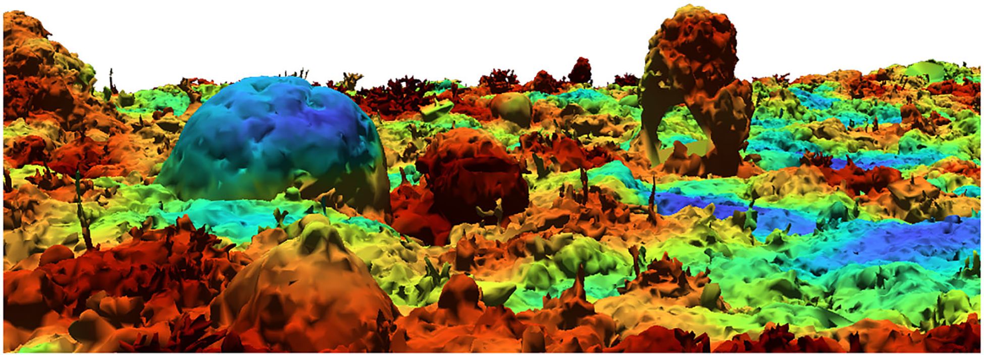
Figure 1. Heatmap of rugosity values on a complex 3D coral reef model.

2 Method

2.1 Algorithm design

Rugosity calculations are generally based on the ratio of triangle area to projected triangle area. Techniques differ in how these calculations are applied (e.g. once globally or multiple times locally), and how the projection vectors, or reference planes, are determined.

To produce rugosity maps, it is necessary to split up models into smaller regions, within which rugosity calculations can be performed locally, and to determine appropriate reference planes for each region. Most existing techniques assume input models are similar to 2.5D height maps and use 2D grids to subdivide them for local rugosity calculations. 2D gridding does not extend well to complex 3D models, where surfaces can be above or below each other.

To handle such multiple surfaces, and the many other edge cases encountered in arbitrary 3D models, we subdivide models into a regular 3D grid of voxels (volume elements), through a process called voxelization: Each triangle of the model is checked to see which voxel(s) it intersects, and each voxel stores a list of triangles that fall at least partially inside. Rugosity is then calculated locally for each voxel.

2.1.1 Reference plane fitting

For projected-area rugosity calculations, an appropriate reference plane must be chosen for each voxel. Slope fitting approaches have been suggested, e.g. the arc–chord ratio (ACR) rugosity index (Du Preez, 2015). However, such methods use 2.5D elevation grids, and thus cannot accommodate complex 3D models with overlaps/overhangs, which are typical in coral reef models and areas with macroalgae.

A straightforward (and fast) method for choosing a reference plane is to use the average surface normal of the voxel’s triangles. The surface normal is a vector extending outwards from, and perpendicular to the surface. While SfM models often have fairly consistent triangle size, filled-holes and peripheral areas can have inconsistently large triangles. To account for this, and to accommodate the widest range of possible 3D models, it is important to weight the normal of each triangle by that triangle’s area. (Likewise, a triangle’s area is also used to weight its contribution to the final value of a voxel.)

Testing with various 3D models revealed occasional instances of unreasonably high rugosity values, due to a variety of edge-cases where reference planes determined by average surface normal were a poor fit for projecting the triangles in a voxel. An example edge case is shown in Figure 2, where a voxel contains part of an object with large horizontal surfaces connected by a small vertical edge. In calculating the average surface normal, the upward and downward normals cancel each other out, causing the reference plane to be based on the sideways normals of the relatively small edge surface. Thus, the largest surfaces are projected almost perpendicularly, resulting in exceedingly-high rugosity values that do not accurately represent the roughness of the surfaces in the voxel.

Figure 2

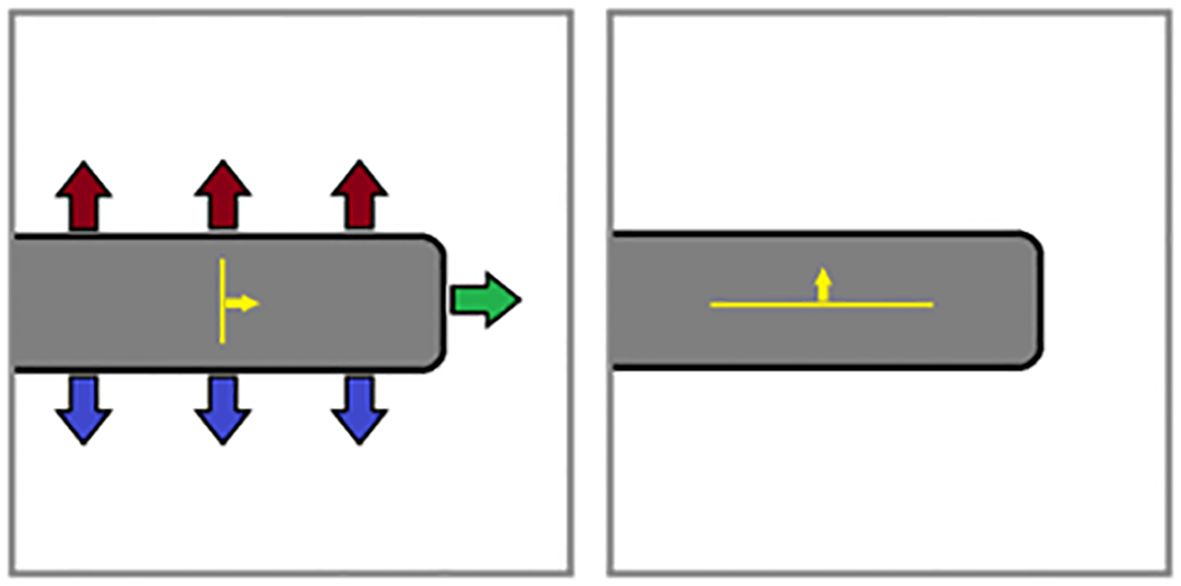
Figure 2. Example problematic edge case; (left) poorly-fit reference plane (yellow) based on average surface normal; (right) more-appropriate reference plane generated using least squares fitting.

In pursuit of more reliably appropriate reference planes, we experimented with alternatives to average surface normal. For example, our software includes an option to calculate reference planes using linear least squares fitting, which computes the best fitting plane for a set of triangles by minimizing the sum of squared distances from triangle vertices to the plane. While this method does generate more-appropriate reference planes in many of the situations in which average normal fails (e.g. Figure 2), our testing showed there were still occasional instances of unreasonably-high rugosity values. Given the relative rarity of these cases within an entire model, we provide the option to automatically remove egregious outlier (>99^th percentile) per-triangle rugosity values when calculating per-voxel rugosity values.

Additional experimentation with using mesh simplification algorithms to determine reference planes is described in the Supplementary Materials.

2.1.2 Rugosity-minimizing technique

Our rugosity minimizing technique finds the optimal reference plane for a voxel by projecting the area of the triangles in that voxel onto many possible reference planes, in every orientation, and choosing the reference plane that produces the lowest total rugosity value. (Complete algorithm available in Supplementary Material B.1, and C++ implementation available on GitHub [https://github.com/Azzinoth/HabiCAT3D]).

This approach was taken because dividing complex 3D models into an arbitrary 3D grid can result in a variety of unpredictable problematic edge-cases, in which triangles are not cleanly arranged in such a way that a single plane can be easily fit. Further, the lowest rugosity value presents as an appropriate reference plane as it produces reasonable rugosity values that are in the range of traditional methods (e.g. tape-and-chain), and scale with increasing surface complexity. Inappropriate reference planes result in rugosity values that are too high. It follows then, that the optimal reference plane for an arbitrary set of triangles is that which minimizes the rugosity value and maximizes the projected area.

Though this method is more computationally intensive than fitting and calculating rugosity for a single plane, it virtually eliminates unreasonably high rugosity values, and produces a tighter, more natural distribution of values. Computational cost (time required), however, can easily be tuned by adjusting the number of possible reference plane orientations, which we generate by uniformly distributing the desired number of points on a unit hemisphere.

As models increase in complexity with multiple overlapping surfaces, traditional projected triangle area rugosity calculation becomes less effective at properly capturing the increased complexity. This is because the projected triangles begin to overlap on the reference plane. To correctly calculate rugosity on such complex models, instead of dividing the total area of the triangles by the total projected area of the triangles, it should be divided by the total unique projected area of the triangles. Our software implements this using CPU-intensive polygon set operations that significantly increase calculation time. Thus, “unique projected area” is provided as an optional feature to be used for very complex models with many overlapping features. (Detailed algorithm available in Supplementary Material B.2.) Relative performance of these options is evaluated in Section 3.1.

2.1.3 Voxel size

Voxel (grid cell) size has a significant impact on 3D gridded rugosity calculations (see Figure 3). Selection of voxel size is further complicated by the fact that there is no single correct size to use for a particular model. Voxel size should be decided based on model resolution and the model’s contents, specifically the size of the features of interest. For large models, voxel size may be limited by computing resources (system memory).

Figure 3

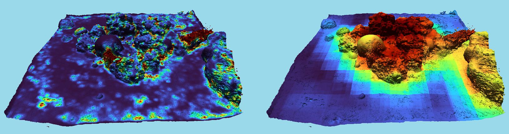
Figure 3. Rugosity maps for the same model, calculated using small (left) and large (right) voxels.

A good guideline is to use a voxel size at least 3x the width of the features of interest. For example, on a model with bumpy features around 10cm wide, try a voxel size around 30cm. Too small of a value will analyze pieces of those bumps, which might individually be smooth; too large of a value will blend larger regions together, reducing the resolution of the resulting rugosity map, and may result in voxels too large to be well-fit by a single reference plane.

It can be helpful to run rugosity calculations more than once, at different voxel sizes, to determine which size best captures your features of interest and reveals the desired level of detail. A multiple-layering system is provided to help switch between and compare the results of different settings. When comparing multiple sites/models to each other, it is best to use a consistent voxel size.

With larger voxel sizes, boundaries between high- and low-rugosity regions will rarely match voxel boundaries, and thus there can be “edge” voxels containing both, resulting in medium-rugosity values. We minimize these unpredictable effects by performing the voxelization and analysis process many times, jittering the voxel grid a small distance in various directions each time. (Detailed jittering algorithm available in Supplementary Material B.3, and C++ implementation available on GitHub.) Each triangle’s final rugosity value is calculated based on the values of all these separate analysis runs. This suppresses problematic edge cases and provides smoother heat maps (see Figure 4).

Figure 4

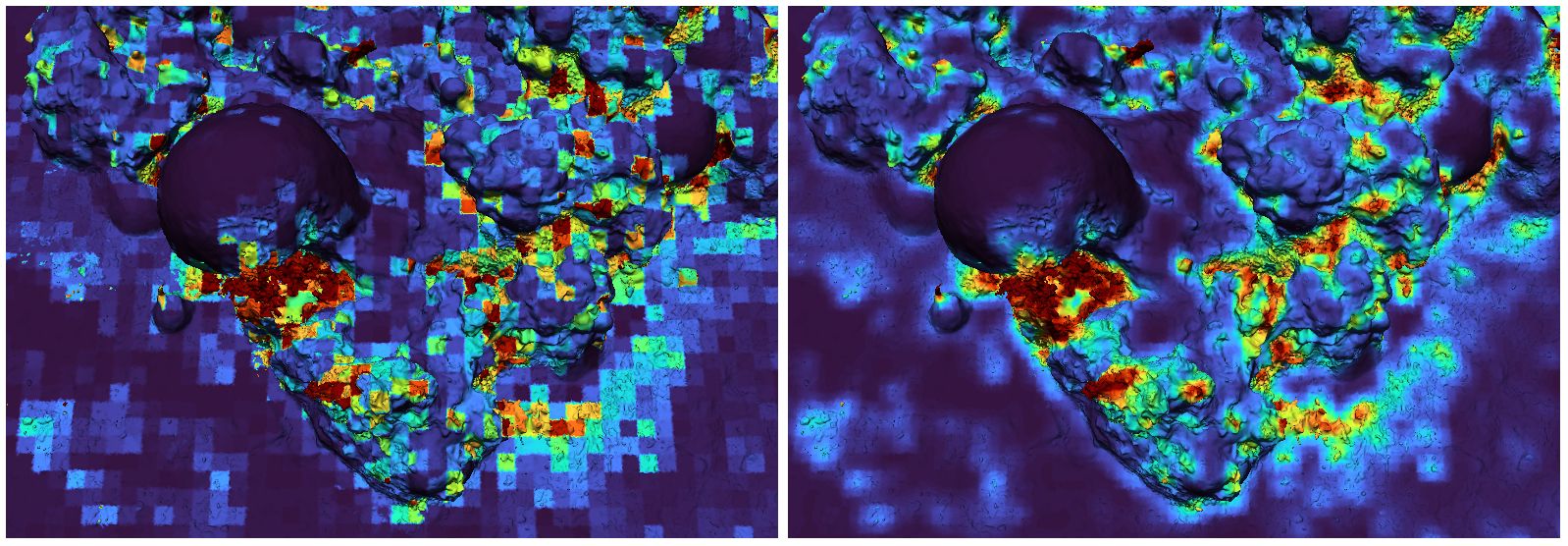
Figure 4. Rugosity heatmaps, showing the blocky results of a single analysis run (left) and the smoother results obtained with multiple analysis runs on jittered grids (right).

2.1.4 Fractal dimension

Beyond rugosity, our voxelization approach can be similarly applied to extend to other complexity metrics. For example, fractal dimension (FD) has long been used, in various forms, to analyze corals and reefscapes. Initially, FD measurements were conducted in 1D (along a line) over a reefscapes (Bradbury and Reichelt, 1983). This progressed to measurements on 2D slices of individual corals (Martin-Garin et al., 2007). More recent approaches calculate FD using a 2.5D rasterized grid of height values derived from a 3D model (Young et al., 2017; Fukunaga et al., 2019). However, as illustrated in Figure 5, collapsing a complex 3D model with overlapping surfaces to 2.5D causes a loss of information and inaccurate results.

Figure 5

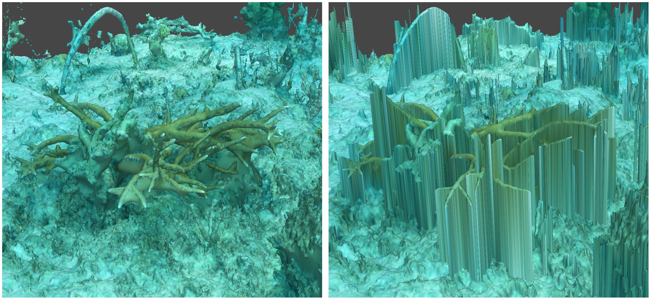
Figure 5. (left) complex 3D coral model, (right) same model collapsed to 2.5D, losing internal details.

Our software calculates local FD values separately for each voxel, using the box counting method (Liebovitch and Toth, 1989). Like the previous rugosity calculations, FD results from each jittered voxel are applied to the associated individual triangles to produce 3D heatmaps.

In addition to properly handling arbitrary complex 3D models, our voxelization approach also provides flexibility in terms of scale: Most existing FD approaches calculate a single FD value for an input model. Thus, they can either generally characterize an entire reef, or individual corals must be extracted and processed separately. Our algorithm can localize FD calculations across the entire model to produce heatmaps illustrating the distribution of FD values at various locations (see Figure 6). Most notably, it decouples the scale of FD calculations from the scale of the input model.

Figure 6

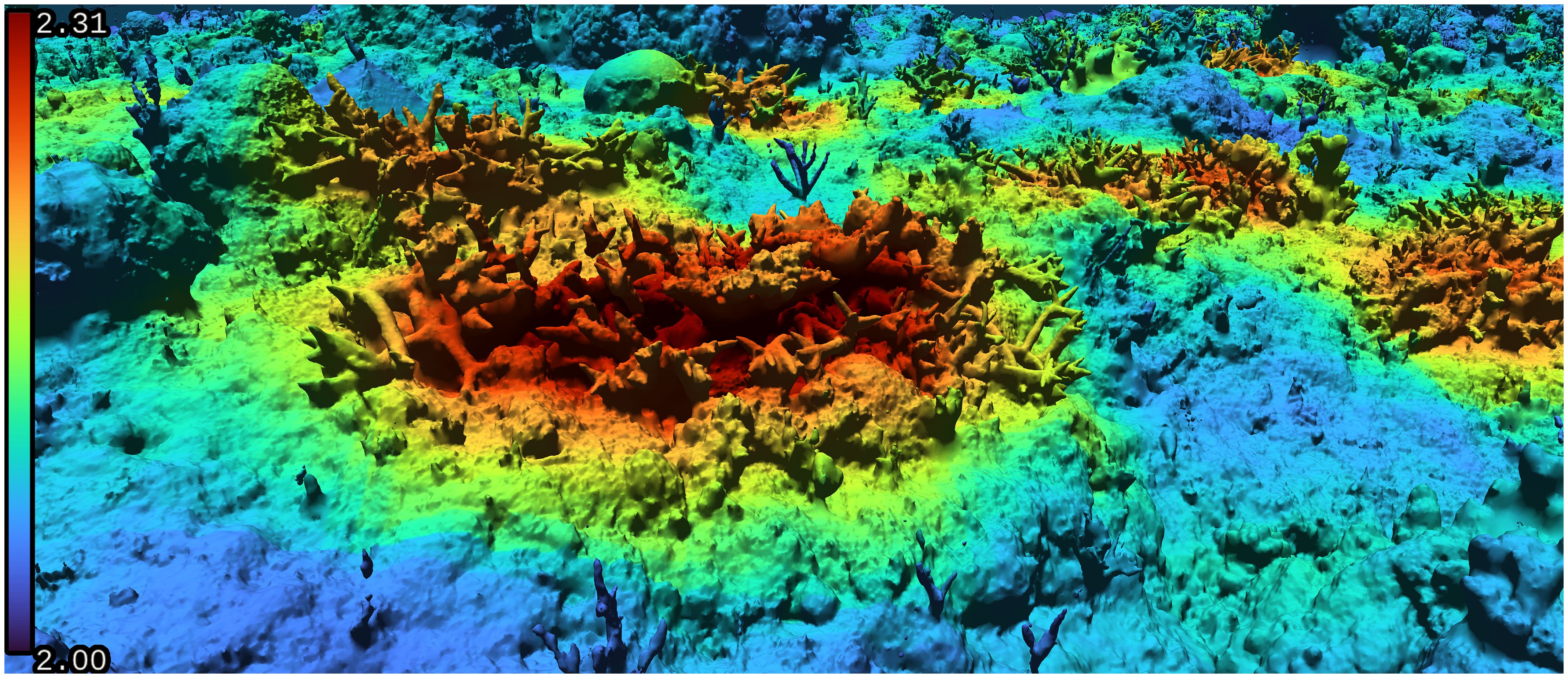
Figure 6. Heatmap of fractal dimension values on a coral reef model. Note the high values inside the staghorn corals, which cannot be adequately captured by 2.5D methods.

Researchers using FD for coral analysis sometimes assert that FD values should fall between two and three (Young et al., 2017). Conceptually, this range is logical, with a value of two representing a plane, and three, a solid cube. However, this assumes input models with surfaces that fully cover grid cells (in x/y), without holes or ragged boundary edges. While this can be assumed for models collapsed to 2.5D heightmaps, real-world SfM models are rarely so clean. Additionally, jittering the analysis grid guarantees that it will not always align with the edges of the model. Consequently, FD values slightly lower than two may occasionally be seen, most often around boundary edges. Our application provides an option to exclude individual values under two when calculating the final FD values of triangles. Tests indicate this affects only very small portions of most models (~0.1% - 0.7%), primarily around boundary edges.

2.2 Application

The algorithms described in this paper have been implemented in an open source, user-friendly (HabiCAT 3D) application, provided for free through GitHub [https://github.com/Azzinoth/HabiCAT3D]. The repository contains the complete source code, along with documentation, build instructions, and dependencies required to compile and run the application. Also, it offers a release section, allowing users to easily download a fully functional version of the application without the need for compilation.

The application provides both a graphical user interface (GUI) and a command-line interface (CLI) with script execution, facilitating integration into existing research workflows. This section outlines the major features of the GUI version; examples and guidelines on how to use the CLI and scripting features can be found in the GitHub repository’s documentation.

The GUI uses a layer system, which enables comparison of results obtained with different techniques and settings. Similar to web-browser tabs, users can switch between, visually compare, and calculate differences between analysis runs.

Analysis results (and other data layers) are visualized as heatmaps on the model. The Turbo colormap (Mikhailov, 2019) provides the look of a traditional rainbow colormap, but with modifications to address perceptual issues (e.g. introduction of false detail).

The application supports loading 3D models in the common Wavefront (.OBJ) format, and can save/load entire workspaces using a custom format. Upon loading, orientation is estimated and a height layer generated. Analysis layers (rugosity, FD, etc.) can then be added, with desired settings. Rugosity settings include voxel size, reference plane determination method, outlier removal, and jitter count.

2.2.1 Recommended settings

The most important setting for rugosity calculations is voxel size (see Section 2.1.3). Based on model size, “small” and “large” options are suggested, or users can specify a custom value. To quickly experiment with a range of sizes, calculate multiple times using “average normal” and the lowest jitter count (7) until features of interest are revealed; then re-run with “rugosity minimizing” and more jitters to achieve results that are smoother and more accurate.

The most significant performance impacts (time and memory required) are from the minimizing function and jittering, as each perform calculations repeatedly. The minimizing function evaluates rugosity using a number of potential reference planes, and is that many times slower than “average normal”, which calculates rugosity once with a single reference plane.

Figure 7 shows the results of testing the minimizing function with different settings on a variety of coral models (some made by Pierce, 2020). A significant, steep drop in rugosity values can be seen between using a single reference plane (average normal) and minimizing using just nine reference planes, indicating the minimizing technique effectively suppresses extreme values resulting from poorly-fit reference planes (see Section 2.1.1). Testing additional reference planes showed diminishing returns, with rugosity values largely stabilizing beyond ~91 planes (our default recommended setting).

Figure 7

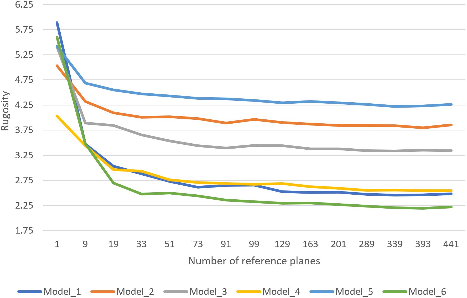
Figure 7. Average rugosity values for various coral models, using the minimizing technique with increasing numbers of possible reference planes.

Similarly, we evaluated the number of jitters required to suppress poor results and produce smooth results. For various coral models, rugosity was calculated using a range of jitters, from 1 (no jittering) to 73 jitters. Figure 8 shows the resulting average rugosity values, revealing that only a few (7) jitters are required to effectively suppress unreasonably high rugosity values from problematic grid cell placement. However, to produce smoother results, a much higher number of jitters is required (we recommend 55). Figure 9 illustrates the visual quality obtained by increasing number of jitters. Models that were used to create graphs can be downloaded from: https://ccom.unh.edu/vislab/downloads/RugosityModels.zip

Figure 8

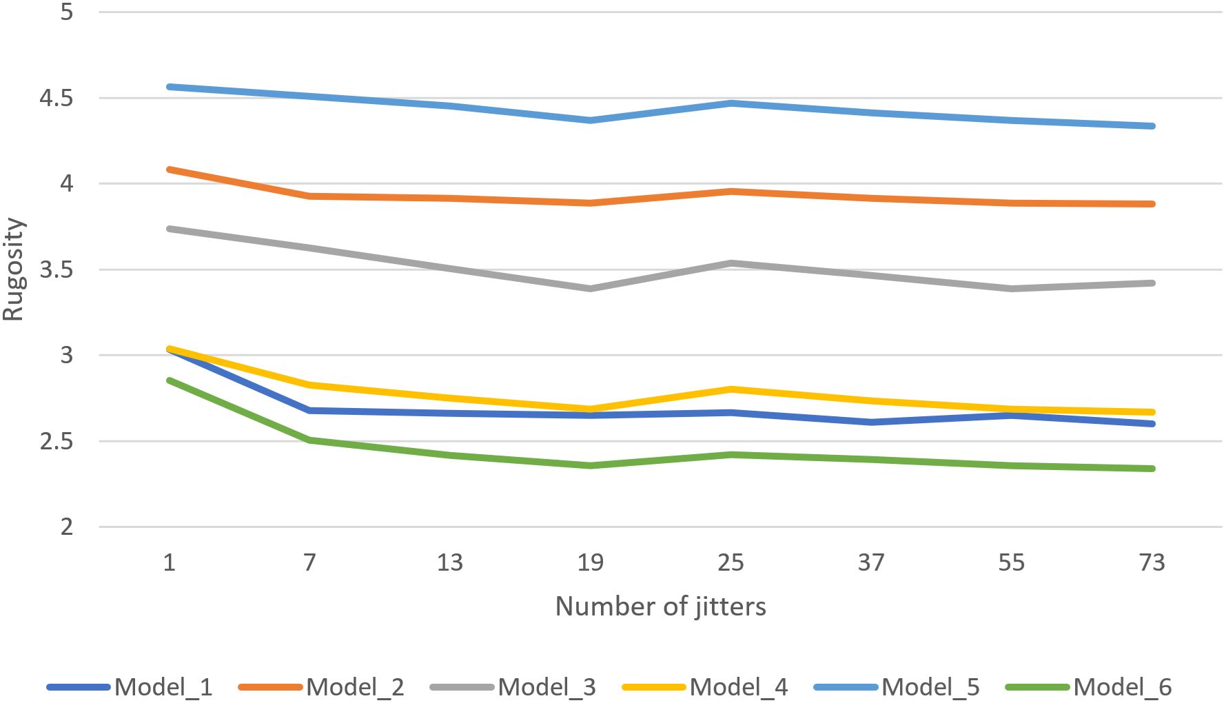
Figure 8. Effect of jitter count on average rugosity values for various coral models.

Figure 9

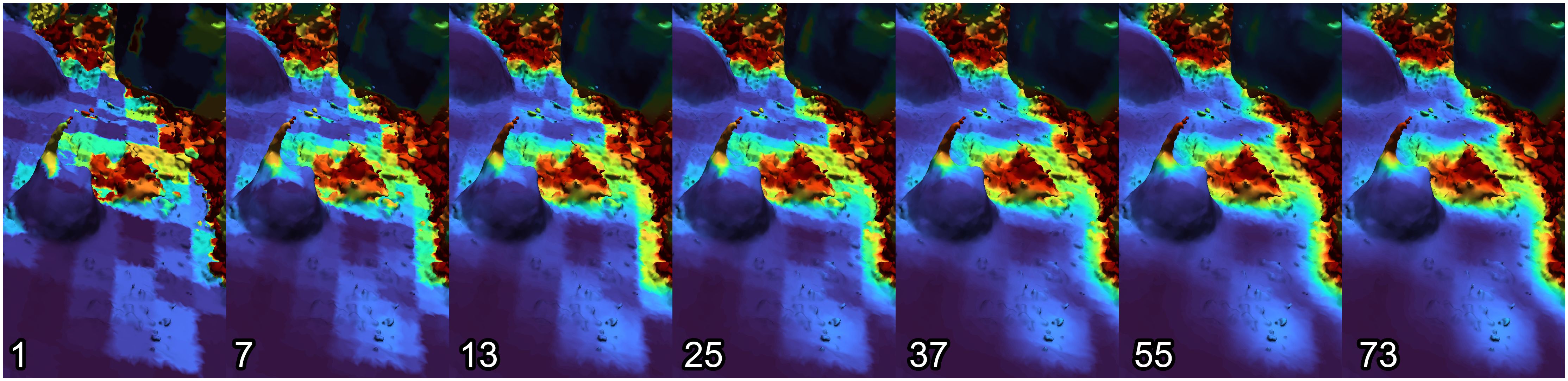
Figure 9. Rugosity heatmap quality improvements with increased jitter counts (1-73).

2.2.2 Additional tools

Interactive histograms (shown in Figure 10) provide deeper insight into the distribution of complexity metrics across the model. At a glance, it is possible to quickly evaluate the uniformity or concentration of complexity in a model. Histogram granularity can be adjusted by setting the number of bins, and interpolation can be toggled between “bar-chart” style and continuous line graph.

Figure 10

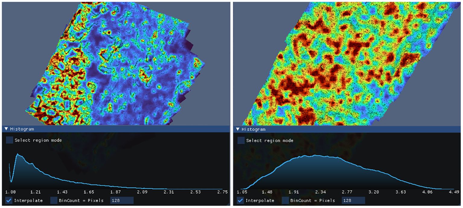
Figure 10. Histograms showing unique rugosity distributions between two models.

Histograms can be queried by mouse to calculate how much surface area falls within a complexity range. As shown in Figure 11, regions corresponding to selected ranges are highlighted to aid correlating the histogram to the model.

Figure 11

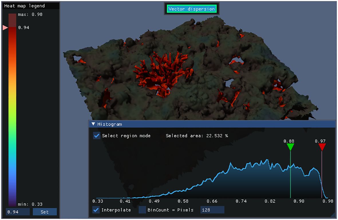
Figure 11. Calculating the surface area within a selected complexity range.

Export tools help extract and save the results of calculations: Selection tools query rugosity (or other values) of a single triangle, or within a radius of a point. Export to File automatically saves coordinates and results of queries to a text file. Screenshot generates figures (PNG) of the model view along with the current color scale.

While the results of our techniques are best viewed and analyzed in 3D, many existing ecological analysis workflows rely on 2D/2.5D representations. HabiCAT 3D can export any data layer to a 2D image representation (e.g. GeoTIFF) suitable for these workflows. This export feature projects 3D data layers along a chosen axis, effectively creating meaningful 2D representations of the layer contents, which can bridge the gap between the advanced 3D capabilities of our software and traditional 2D approaches.

Exports can be PNG or GeoTIFF format, with the latter supporting 32-bit float format for outputting raw complexity values instead of color-scaled heatmaps.

When projecting values on a 3D model to a 2D image, multiple triangles may project to the same pixel. Four options are provided to resolve this: min, max, mean, or cumulative. The first three are self-explanatory, while the cumulative option accumulates the complexity metric of all triangles along the projection axis. The resulting image can be thought of as an “X-ray” of the 3D model, which preserves information about the complexity of multiple overlapping surfaces in a 2D representation. This mode is particularly useful for complex models with overhangs and caves.

3 Results

3.1 Relative metric performance

We can extend rugosity calculations to complex 3D models, but is this traditional metric the most appropriate for such datasets? We implemented two competing complexity metrics, fractal dimension and vector dispersion to evaluate how each performs with increasingly complex 3D coral models.

Three test models are shown in Figure 12. The first is a snippet of a larger reef model, containing a staghorn coral and seafloor. The second is the same model, with the coral cloned twice (and rotated) to create a larger, denser coral (3x branches). The third model has the coral cloned four times (5x branches), creating an extremely dense coral with complex internal detail.

Figure 12

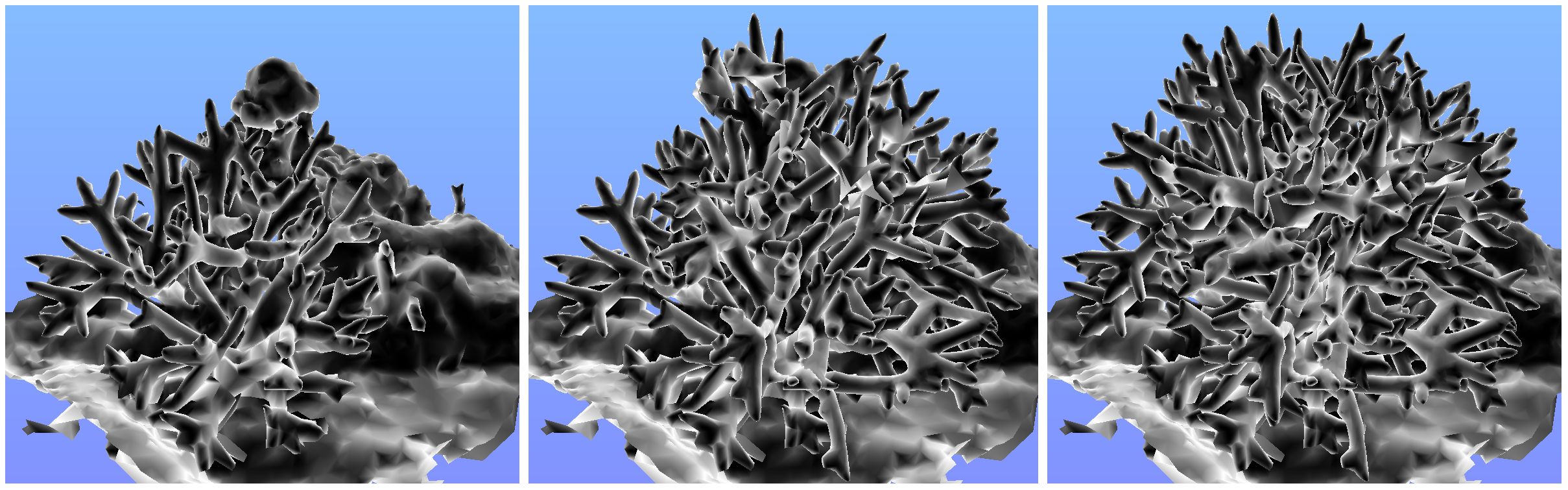
Figure 12. The test models: (left) one coral, (middle) 3x corals superimposed, (right) 5x corals superimposed.

Figure 13 shows the results of each complexity metric calculated on each model as a whole, mirroring how such analysis is often done on single corals. Rugosity, calculated using minimizing and “unique projected area” (slow, but recommended for models with many overlapping features), exhibited the highest correlation with the linearly increasing model complexity (number of superimposed corals). Rugosity, calculated using the (much faster) non-unique minimizing technique did not increase at the same linear rate, but still adequately captured the increasing complexity.

Figure 13

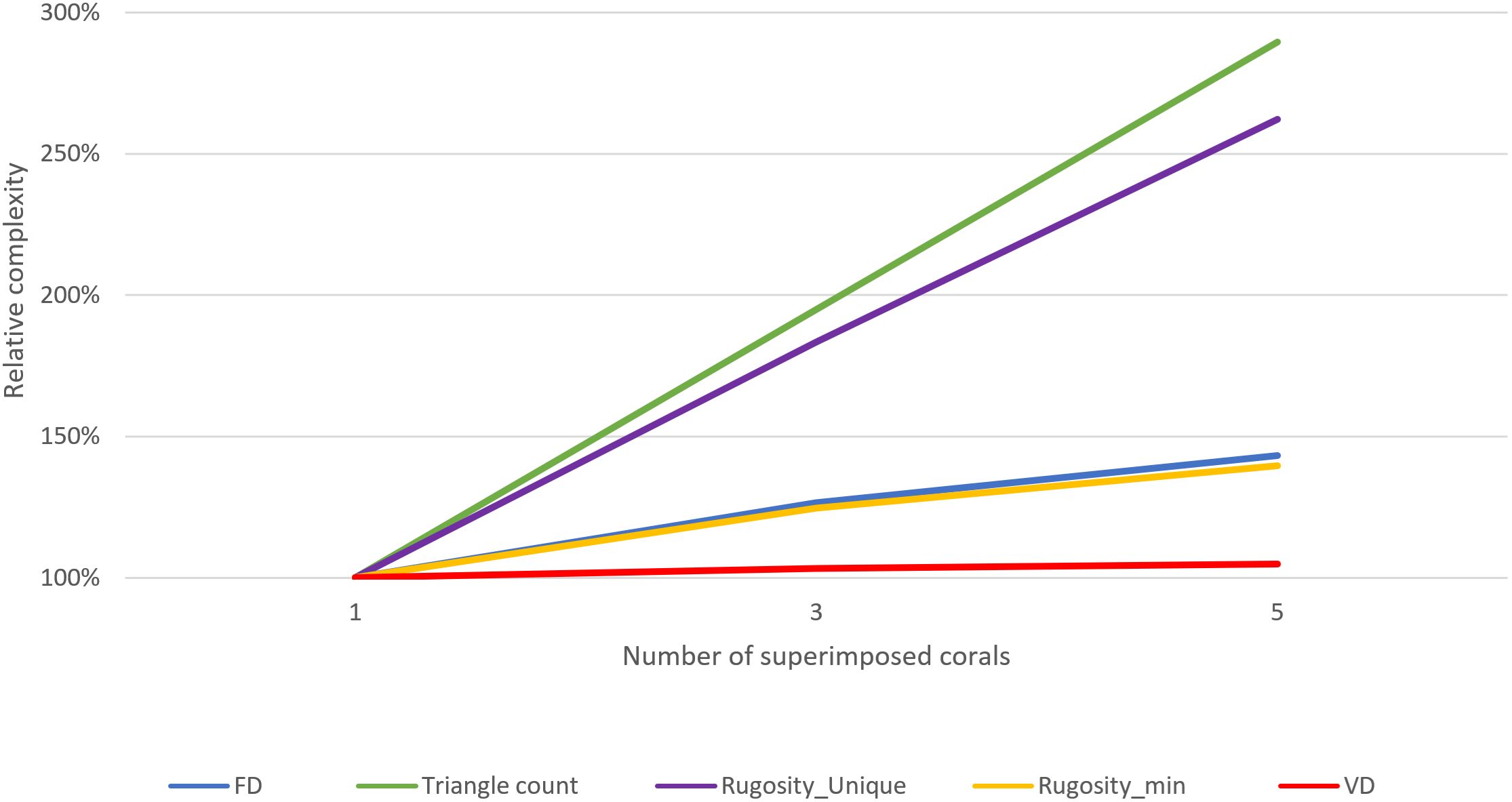
Figure 13. Results of various complexity metrics on increasingly complex coral models.

Fractal dimension performed almost identically to non-unique rugosity-minimizing rugosity, effectively capturing the increase in complexity, but not linearly; which is to be expected, as FD has a maximum value of three that it asymptotically approaches (whereas rugosity has no upper bound).

Vector dispersion predictably failed to capture the increasing complexity, having already almost reached its maximum value (1.0) with the original model, leaving little room to increase along with model complexity. This low dynamic range of vector dispersion makes it ill-suited for even mildly complex models, and we do not recommend its use.

How do these techniques perform on the same models when performed across the model at a finer scale (~16x16x16 grid) using our voxelization technique? Figure 14 shows the resulting mean values of the different complexity metrics when performed across models with a finer scale (16x16x16 grid).

Figure 14

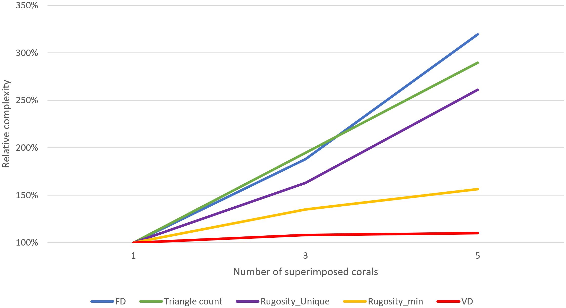
Figure 14. Results of various complexity metrics using our voxel grid approach.

Fractal dimension values increased significantly faster than the previous analysis; while overshooting slightly, they more effectively captured the true increase in complexity, now that the FD analysis window is smaller than the entire model. Smaller analysis windows translate to smaller scales in the underlying FD box-counting calculations, which more tightly fit the contents of the model (ignoring more empty space) and better match the small, detailed branches in the models.

Rugosity, calculated with unique projected area, again increases linearly along with model complexity. However, values are now lower, as multiple analysis cells generate better-fitting reference planes for each local area. Minimizing rugosity without unique projected area lagged below the increase in model complexity, which is expected for such a complex model with many overlapping surfaces.

Our evaluations of the various complexity metrics suggest that both rugosity and fractal dimension are useful metrics for quantifying the relative complexity within 3D models. When used with our jittered voxelization technique, both can be extended to produce 3D heatmaps of values across complex 3D models. Fractal Dimension in particular benefits greatly from being performed locally at smaller scales, where box counting sizes can more closely match the features in the model, irrespective of the overall scale of the model itself. This means a large model with multiple corals can be analyzed all at once, without having to cut individual corals out for separate analysis. For extremely complex models, FD can provide faster results than the costly unique projected area algorithm required to get accurate rugosity values on such models.

3.2 Practical application

We explored the practical benefits of applying our techniques to an ecological study, in which Dyson (Dyson, 2023) used fine-scale seafloor data and advanced digital modeling to identify optimal locations for staghorn coral outplanting, with specific emphasis on using fine-scale metrics. Dyson digitized previously outplanted sites into raster height maps (DEMs) and orthomosaics using photogrammetry, and the outlines of corals of interest were hand-traced into vector (shapefile) region masks. These outlines were dilated to create region masks of the seafloor immediately surrounding, but not within, each coral (see Figure 15A). Metrics, including complexity, were calculated on a DEM of the entire site, and the masks were used to extract subsets of resulting values immediately surrounding (but not within) each coral. These values were evaluated to discover correlations with observed health of each coral. Of the various 2.5D complexity metrics evaluated in Dyson’s study, arc–chord ratio (ACR) rugosity index (Du Preez, 2015) showed the highest correlation with coral health. Thus, we used the results of arc–chord rugosity on DEM as a baseline.

Figure 15

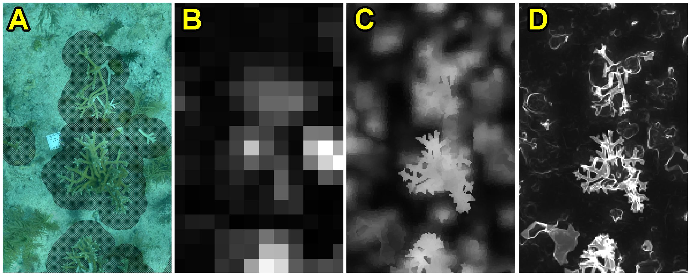
Figure 15. (A) Orthomosaic with region masks around corals; (B) ArcMap arc–chord rugosity map; (C) our rugosity map, exported using max; (D) our rugosity map, exported using cumulative; (B–D) all use the same 10cm analysis window size, but jittering and per-triangle results provide finer detail in (C) and (D).

To our knowledge, there is currently no available one-button solution to calculate arc-chord rugosity. We used ArcMap with an extension.

We loaded a 3D model generated from the same photogrammetry data as the DEM, and applied our rugosity-minimizing technique with a 10cm voxel size (matching the 10cm window size of the arc-chord analysis), and 55 jitters. The results were output as a 32-bit GeoTIFF, a 2D data product that could be inserted into the existing GIS-based workflow.

In addition to properly accounting for the significant 3D details that were lost when collapsing the photogrammetry data to a 2D DEM, there is finer detail in the rugosity maps generated using our software. See Figure 15 for a visual comparison of the data products, all calculated using the same 10cm analysis window size. The blocky vs smooth appearance of the seafloor between Figures 15B, C results from the multiple, jittered runs. (Arc-chord results could potentially be similarly improved if run multiple times with jittering, but no software to do this currently exists.) However, an important distinction is the sharp outlines of the staghorn corals themselves. Because our software stores the results of the 3D analysis per-triangle, it can preserve 3D details even in 2D exports. It is important to note that export resolution is independent of analysis voxel size, i.e. while the analysis voxel size was 10cm, results can be output in much finer detail (e.g. cm scale).

The rugosity maps generated using our application provide finer details, and a clear separation between corals and seafloor. This has significant impact on the effectiveness of the existing research workflow: Though the corals were carefully traced to exclude them from their surrounding regions, the height values within coral outlines still had an effect on the arc-chord results outside those outlines. Because our method analyzes the model in 3D, the protruding corals are processed separately from the seafloor, and this separation can be maintained in the results. Furthermore, our software was able to account for the complex 3D details present in the photogrammetry data/model, which were lost when collapsing it to a DEM.

3.3 Mesh quality and processing considerations

The sensitivity of complexity metrics to mesh quality and post-processing operations is an important consideration for practical applications. We evaluated these effects using 17 test models, focusing primarily on rugosity analysis. While our findings should generally apply to other complexity metrics, some specific considerations for FD calculations are discussed below.

Our software was designed to handle uncleaned meshes with various topological issues, but to quantify the impact of common mesh cleaning operations, we used MeshLab v2023.12 (Cignoni et al., 2008) to test the impact of removing: duplicate faces, duplicate vertices, zero-area faces, and T-vertices, as well as repair of non-manifold edges and vertices.

Results showed that mesh cleaning operations had minimal impact on rugosity calculations, with values ranging from 98.8% to 100.3% of the original uncleaned model. This suggests that users can reliably apply our analysis tool to both cleaned and uncleaned meshes, though more extensive testing with other processing tools could further validate these findings. (See Supplementary Material B.4 for a comprehensive breakdown of cleaning operations and their impacts.)

In contrast, remeshing operations showed more substantial effects. Using MeshLab’s Isotropic Explicit Remeshing (Hoppe et al., 1993), rugosity values varied from 86.9% to 114.6% of original values, with visually apparent differences in results exported as images (see Supplementary Material B.5). Based on these findings, we recommend not remeshing models prior to analysis, and caution that results cannot be meaningfully compared between remeshed and original models.

Our algorithms handle incomplete surfaces robustly, so hole-filling operations are not necessary; Furthermore, hole-filling can locally impact complexity measurements, typically reducing both rugosity and fractal dimension values.

Though mesh quality issues from poor photogrammetric reconstruction are not directly related to our analysis methods, our tool can generate a triangle area layer that can be helpful in identification of potentially problematic regions (Supplementary Material B.6), enabling informed decisions about which areas to include in analyses. To help users assess computational requirements, we provide benchmark data in Supplementary Material B.7, including model triangle counts and processing times.

4 Discussion

The popularity of structure-from-motion has led to a proliferation of complex 3D models that traditional habitat complexity metrics struggle to handle properly. Most existing techniques flatten 3D models into 2.5D raster height grids, discarding important structural information. We have presented algorithms for extending the traditional rugosity metric to properly handle complex 3D models with arbitrary orientations, overlapping surfaces, holes, and other complicated features.

By breaking 3D models up into a voxel grid, we can localize rugosity (and other) calculations throughout the model, such that they match local surface orientations, with scales matching features of interest. By performing calculations multiple times while jittering the voxel grid, we can produce smoother results and reduce the impact of rare edge-cases that result in spurious values. Our novel rugosity-minimizing technique avoids the pitfalls of trying to calculate a single representative reference plane for an arbitrary collection of triangles, and instead tests many potential reference planes, selecting the one that results in the lowest rugosity value. This virtually eliminates extreme rugosity values arising from edge cases involving near-perpendicular projection onto poorly fit reference planes generated using traditional methods such as average surface normal.

As both the jittering and rugosity-minimizing techniques involve running calculations multiple times, it is important to understand the cost-benefit tradeoffs. We evaluated the effects different settings had on coral reef rugosity calculations, and identified recommended values that provide sufficient accuracy without wasting computation time on diminishing returns.

We demonstrate how our method can be applied to other complexity metrics, such as fractal dimension (FD) and vector dispersion, to properly handle complex 3D models and produce results in the form of heatmaps covering such models. For FD, localizing and jittering the calculations can separate the scale of the FD calculations from the scale of the model, and provide per-triangle FD values that better represent the distribution of complexity.

Finally, we implemented these techniques in an easy-to-use application that is freely provided via GitHub [https://github.com/Azzinoth/HabiCAT3D]. It provides useful tools for visual analysis of rugosity and FD calculations, and can export results for publication and further analysis. It is our hope that the benthic ecology community will find HabiCAT 3D useful for characterizing the complexity and habitat value of the models they are generating.

Data availability statement

The original contributions presented in the study are included in the article/Supplementary Material. Further inquiries can be directed to the corresponding author/s.

Author contributions

KB: Investigation, Software, Visualization, Writing – original draft, Writing – review & editing, Conceptualization, Methodology, Validation, Data curation, Formal analysis. JD: Conceptualization, Data curation, Writing – review & editing, Writing – original draft, Funding acquisition, Investigation, Methodology, Resources. TB: Conceptualization, Supervision, Visualization, Writing – original draft, Writing – review & editing, Methodology, Funding acquisition, Investigation, Project administration, Resources.

Funding

The author(s) declare financial support was received for the research, authorship, and/or publication of this article. This research was made possible through the support of NOAA Grant NA20NOS4000196.

Conflict of interest

The authors declare that the research was conducted in the absence of any commercial or financial relationships that could be construed as a potential conflict of interest.

Publisher’s note

All claims expressed in this article are solely those of the authors and do not necessarily represent those of their affiliated organizations, or those of the publisher, the editors and the reviewers. Any product that may be evaluated in this article, or claim that may be made by its manufacturer, is not guaranteed or endorsed by the publisher.

Supplementary material

The Supplementary Material for this article can be found online at: https://www.frontiersin.org/articles/10.3389/fmars.2025.1449332/full#supplementary-material

References

AgiSoft MetaShape Professional (2020). AgiSoft MetaShape Professional (Version 1.6) (Software). Available online at: http://www.agisoft.com/downloads/installer/ (Accessed December 15, 2023).

Google Scholar

Bayley D. T., Mogg A. O., Koldewey H., Purvis A. (2019). Capturing complexity: field-testing the use of structure from motion derived virtual models to replicate standard measures of reef physical structure. PeerJ. doi: 10.7717/peerj.6540

PubMed Abstract | Crossref Full Text | Google Scholar

Bradbury R. R., Reichelt R. R. (1983). Fractal dimension of a coral reef at ecological scales. Mar. Ecol. Prog. Ser. 10, 169–171. doi: 10.3354/meps010169

Crossref Full Text | Google Scholar

Cignoni P., Callieri M., Corsini M., Dellepiane M., Ganovelli F., Ranzuglia G. (2008). Meshlab: an open-source mesh processing tool. Eurogr. Ital. chapter Conf. 2008, 129–136. doi: 10.2312/LocalChapterEvents/ItalChap/ItalianChapConf2008/129-136

Crossref Full Text | Google Scholar

Du Preez C. (2015). A new arc–chord ratio (ACR) rugosity index for quantifying three-dimensional landscape structural complexity. Landscape Ecol. 30, 181–192. doi: 10.1007/s10980-014-0118-8

Crossref Full Text | Google Scholar

Dyson G. (2023). Habitat suitability modeling long-term growth and healthy cover trends of staghorn coral (acropora cervicornis) outplants in the lower florida keys. Durham, NH, USA: University of New Hampshire.

Google Scholar

Fukunaga A., Burns J. H., Craig B. K., Kosaki R. K. (2019). Integrating three-dimensional benthic habitat characterization techniques into ecological monitoring of coral reefs. J. Mar. Sci. Eng. 7, 27. doi: 10.3390/jmse7020027

Crossref Full Text | Google Scholar

Gough C. M., Atkins J. W., Fahey R. T., Curtis P. S., Bohrer G., Hardiman B. S., et al. (2022). Disturbance has variable effects on the structural complexity of a temperate forest landscape. Ecol. Indic. 140. doi: 10.1016/j.ecolind.2022.109004

Crossref Full Text | Google Scholar

Hoppe H., DeRose T., Duchamp T., McDonald J., Stuetzle W. (1993). “Mesh optimization,” in Proceedings of the 20th annual conference on Computer graphics and interactive techniques. 19–26. (New York, NY, United States: Association for Computing Machinery) doi: 10.1145/166117.166119

Crossref Full Text | Google Scholar

Jackson T. D., Williams G. J., Walker-Springett G., Davies A. J. (2020). Three-dimensional digital mapping of ecosystems: a new era in spatial ecology. Proc. R. Soc. B 287. doi: 10.1098/rspb.2019.2383

PubMed Abstract | Crossref Full Text | Google Scholar

Liebovitch L. S., Toth T. (1989). A fast algorithm to determine fractal dimensions by box counting. Phys. Lett. A 141, 386–390. doi: 10.1016/0375-9601(89)90854-2

Crossref Full Text | Google Scholar

Loke L. H., Chisholm R. A. (2022). Measuring habitat complexity and spatial heterogeneity in ecology. Ecol. Lett. 25, 2269–2288. doi: 10.1111/ele.14084

PubMed Abstract | Crossref Full Text | Google Scholar

Martin-Garin B., Lathuilière B., Verrecchia E. P., Geister J. (2007). Use of fractal dimensions to quantify coral shape. Coral Reefs 26, 541–550. doi: 10.1007/s00338-007-0256-4

Crossref Full Text | Google Scholar

Mazzuco A. C. D. A., Stelzer P. S., Bernardino A. F. (2020). Substrate rugosity and temperature matters: patterns of benthic diversity at tropical intertidal reefs in the SW Atlantic. PeerJ. doi: 10.7717/peerj.8289

PubMed Abstract | Crossref Full Text | Google Scholar

McCoy E. D., Bell S. S. (1991). Habitat structure: the evolution and diversification of a complex topic. Habitat struct.: Phys. arrange. objects space. 8, 3–27. doi: 10.1007/978-94-011-3076-9_1

Crossref Full Text | Google Scholar

Mikhailov A. (2019). Turbo, an improved rainbow colormap for visualization. Google AI Blog. Available at: https://blog.research.google/2019/08/turbo-improved-rainbow-colormap-for.html (Accessed June 13, 2023).

Google Scholar

Pascoe K. H., Fukunaga A., Kosaki R. K., Burns J. H. (2021). 3D assessment of a coral reef at Lalo Atoll reveals varying responses of habitat metrics following a catastrophic hurricane. Sci. Rep. 11, 12050. doi: 10.1038/s41598-021-91509-4

PubMed Abstract | Crossref Full Text | Google Scholar

Pierce J. P. (2020). Automating the boring stuff: a deep learning and computer vision workflow for coral reef habitat mapping. University of New Hampshire.

Google Scholar

Roberts C. M., Ormond R. F. (1987). Habitat complexity and coral reef fish diversity and abundance on Red Sea fringing reefs. Mar. Ecol. Prog. Ser. 41, 1–8. doi: 10.3354/meps041001

Crossref Full Text | Google Scholar

Smith T. B., Kinnison M. T., Strauss S. Y., Fuller T. L., Carroll S. P. (2014). Prescriptive evolution to conserve and manage biodiversity. Annu. Rev. Ecol. Evol. System. 45, 1–22. doi: 10.1146/annurev-ecolsys-120213-091747

Crossref Full Text | Google Scholar

Stoner A. W., Lewis F. G. III (1985). The influence of quantitative and qualitative aspects of habitat complexity in tropical sea-grass meadows. J. Exp. Mar. Biol. Ecol. 94, 19–40. doi: 10.1016/0022-0981(85)90048-6

Crossref Full Text | Google Scholar

Vierling K. T., Vierling L. A., Gould W. A., Martinuzzi S., Clawges R. M. (2008). Lidar: shedding new light on habitat characterization and modeling. Front. Ecol. Environ. 6, 90–98. doi: 10.1890/070001

Crossref Full Text | Google Scholar

Warfe D. M., Barmuta L. A., Wotherspoon S. (2008). Quantifying habitat structure: surface convolution and living space for species in complex environments. Oikos 117, 1764–1773. doi: 10.1111/j.1600-0706.2008.16836.x

Crossref Full Text | Google Scholar

Wilson S. K., Graham N. A. J., Polunin N. V. (2007). Appraisal of visual assessments of habitat complexity and benthic composition on coral reefs. Mar. Biol. 151, 1069–1076. doi: 10.1007/s00227-006-0538-3

Crossref Full Text | Google Scholar

Yanovski R., Nelson P. A., Abelson A. (2017). Structural complexity in coral reefs: examination of a novel evaluation tool on different spatial scales. Front. Ecol. Evol. 5. doi: 10.3389/fevo.2017.00027

Crossref Full Text | Google Scholar

Young G. C., Dey S., Rogers A. D., Exton D. (2017). Cost and time-effective method for multi-scale measures of rugosity, fractal dimension, and vector dispersion from coral reef 3D models. PloS One 12. doi: 10.1371/journal.pone.0175341

PubMed Abstract | Crossref Full Text | Google Scholar