Enhancing bathymetric prediction by integrating gravity and gravity gradient data with deep learning

This study aims to enhance the spatial resolution and accuracy of bathymetric prediction by integrating Gravity Anomaly (GA) and Vertical Gravity Gradient Anomaly (VGG) data with a dual-channel Backpropagation Neural Network (BPNN). The seafloor topography of the Izu-Ogasawara Trench in the Western Pacific will be constructed and evaluated using depth models and single-beam data. The BPNN improved the accuracy of seafloor topography prediction by 0.17% and 0.35% using the 1 arc-minute SIO and GEBCO depth models, respectively, in areas without in-situ data. When single-beam data was utilized, the BPNN improved prediction accuracy by 64.93%, 70.29%, and 68.78% compared to the Gravity Geological Method (GGM), SIO v25.1, and GEBCO 2023, respectively. When single-beam, GA, and VGG data were all combined, the root mean square error (RMSE) was reduced to 19.12 m, representing an improvement of 60.92% and 61.13% compared to using only GA or VGG data, respectively. Comparing bathymetric predictions at different depths, the BPNN achieved a mean relative error (MRE) as low as 0.5%. Across various terrains—such as trench areas, seamounts, and deep-sea plains—the accuracy of seafloor topography predicted by the BPNN improved by 88.36%, 87.42%, and 84.39% compared to GGM, SIO and GEBCO depth models, respectively. These findings demonstrate that BPNN can integrate GA and VGG data to enhance both the accuracy and spatial resolution of seafloor topography in regions with and without in-situ data, and across various depths and terrains. This study provides new data and methodological support for constructing high-precision global seafloor topography.

1 Introduction

Seafloor topography holds significant value in economic, military, and scientific research. High-precision, high-resolution mapping of the seafloor aids in drilling and extraction activities, reducing risks and costs (Wegner and Campbell, 2014). It helps identify fishing grounds and fish habitats (Sutton et al., 2008), optimizing fisheries management and promoting sustainable development (Lehodey and Grandperrin, 1996). Additionally, it supports submarine navigation, undersea communication cable laying, and the construction of underwater military facilities. Understanding seafloor topography is crucial for clarifying tectonic plate movements, volcanic activity, and seismic mechanisms, revealing Earth’s history and evolutionary processes. Moreover, it affects physical processes such as ocean circulation (Noei et al., 2018), tides (Schorghofer, 2010), and waves, thereby influencing global climate and weather patterns. Thus, high-precision, high-resolution seafloor topography is vital for understanding Earth’s evolution, global climate change, and the structure and function of marine ecosystems, while also playing a crucial role in economic development and national security.

The Earth’s oceans cover approximately 360 million square kilometers, accounting for about 71% of the Earth’s surface. Traditional seafloor mapping primarily relies on single-beam and multi-beam sonar technologies. While these methods provide precise measurements, they have limited coverage and are costly (Smith, 2004). Additionally, the varying ocean depths—from shallow to deep waters—and the complex and diverse topographies increase the difficulty of measurements. Consequently, obtaining high-resolution global seafloor topography using traditional methods is challenging. With the continuous advancement of satellite altimetry, the accuracy and density of altimetric data have improved, prompting researchers to explore altimetry-derived gravity inversion for seafloor topography studies. Parker presented the first accurate theory for calculating gravity anomalies due to seafloor topography using the Fast Fourier Transform, which takes into account the non-linear effects of topographic roughness (Parker, 1973). Watts analyzed the gravity and bathymetry relationship for 14 profiles of the Emperor Hawaiian Seamount chain using cross-spectral techniques to obtain a derivative function between gravity and bathymetry (Watts, 1978). Currently, traditional methods for gravity inversion of seafloor topography include the Smith and Sandwell method (Smith and Sandwell, 1994, 1997), least squares collocation (Calmant, 1994; Fan et al., 2021; Tscherning, 1994),and the gravity-geological method (GGM) (Hsiao et al., 2011; Kim et al., 2010; Xiang et al., 2017).

Artificial intelligence (AI) technologies have emerged. AI’s massive data processing algorithms have been widely applied in fields such as seismology, geophysics, and geochemistry, achieving significant results. Researchers have attempted to use AI for altimetry-derived ocean gravity data inversion and to integrate multi-source bathymetric data to construct global bathymetric models. For example, Jena et al. used artificial neural networks to invert the bathymetry of the Arabian Sea, achieving depth inversion accuracy better than 150m for 94% of the area and better than 50m for 2% of the area (Jena et al., 2012). Yang et al. compared fully connected deep neural networks and convolutional neural networks with the GGM to determine if deep learning could provide better seafloor topography predictions. They used short-wavelength gravity and geological models as training parameters and evaluated the performance of different models and parameter combinations. The results indicated that the fully connected deep neural networks method had the highest accuracy (Yang et al., 2023). Zhang et al. applied machine learning techniques based on the Smith and Sandwell method to establish new mathematical relationships. The improved SAS method combined the Genetic Algorithm-back propagation algorithm to invert the topography of the Scarborough Seamount Chain in the South China Sea. The results showed that the Genetic Algorithm-back propagation algorithm method significantly reduced residuals and improved the accuracy of the Smith and Sandwell method inversion method (Zhang et al., 2024). Harper et al. designed and trained a neural network using a dataset of 50 million depth measurements to predict global bathymetry (Harper and Sandwell, 2024).

Many scholars believe that vertical gravity gradient (VGG) contain more short-wavelength information about seafloor topography, supporting the feasibility of using these anomalies to predict bathymetry. Wang explored an alternative technique using VGG, based on the observation that these anomalies primarily originate from localized mass concentrations on the seafloor, with negligible influence from the mass compensation of the oceanic crust. This approach generates bathymetric predictions independent of isostatic modeling assumptions, providing constraints for lithospheric compensation models and other geodetic and geophysical applications (Wang, 2000). Wan et al. studied the sensitivity of gravity anomalies (GA) and VGG in bathymetric inversion. Their results showed that VGG are more sensitive to short-wavelength signals than gravity anomalies, especially in the 0-20 km wavelength range (Wan et al., 2019). Therefore, combining GA and VGG can improve seafloor topography prediction.

A dual-channel Backpropagation neural network (BPNN) has strong nonlinear mapping capabilities, effectively modeling various geophysical transfer functions, such as the relationship between gravity anomalies and bathymetry. BPNN can integrate GA and VGG for depth inversion without mutual interference. Sun et al. introduced dual-channel BPNN into bathymetric prediction, proposing a method based on GA and VGG for depth estimation. By comparing neural networks with gravity-geological methods, they found that the neural network approach offered higher accuracy, confirming the feasibility and effectiveness of the BPNN method (Sun et al., 2022). Most of these studies focus on areas with dense ship-measured bathymetric data. This paper addresses how to improve the accuracy of seafloor topography in regions lacking such data.

The Izu-Ogasawara Trench (26°N–34°N, 140°E–148°E) is located in the western Pacific Ocean, connecting to the Japan Trench in the north and the Mariana Trench in the south (Figure 1). This region features complex and rapidly changing topography, including abyssal plains, seamounts, and trenches, with depths reaching up to 9,780 meters. It provides an ideal setting to evaluate the performance of neural network models for bathymetric inversion under various depth and terrain conditions.

Figure 1

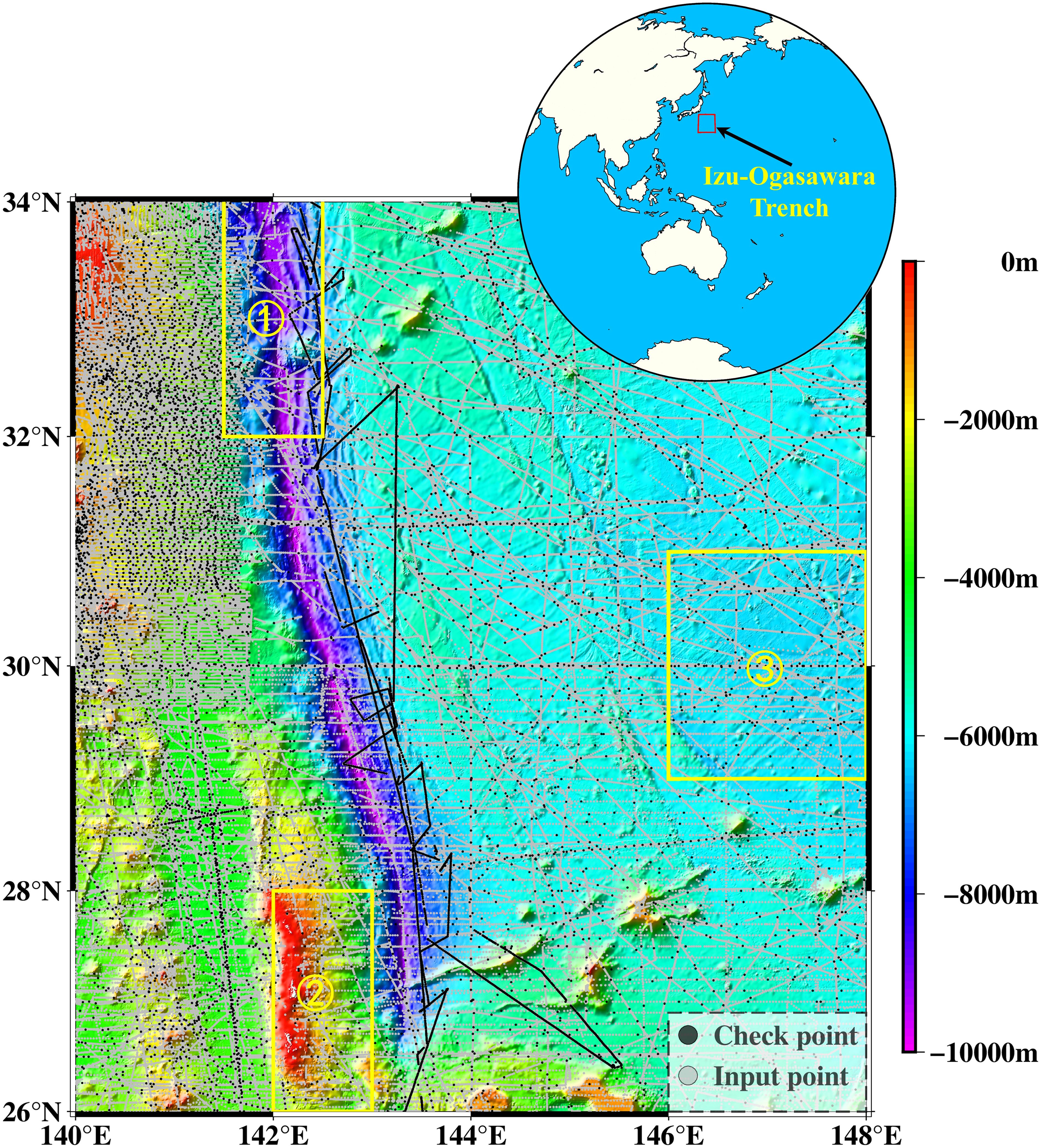
Figure 1. Study area and distribution of shipboard data. Black dots represent checkpoints, and gray dots represent input points. The regions include: ①Trench Area, ②Seamount Area, ③Abyssal Plain Area.

This study uses the BPNN to integrate GA and VGG for predicting the seafloor topography of the Izu-Ogasawara Trench. The performance of this method in bathymetric inversion is evaluated through the following: 1) To evaluate the performance of the model in inverting seafloor topography by using bathymetric models with different spatial resolutions and single-beam data; 2) To verify the effectiveness of gravity data integration, three input data scenarios are designed: GA, VGG, and combined GA and VGG; 3) To assess the adaptability of the model, its performance in predicting bathymetry is compared with the GGM and other bathymetric models under various depth and terrain conditions.

2 Data and methods

2.1 Data

The data used in this study includes:

1. GA and VGG are the 1 arc-minute resolution data from version 32.1, downloaded from the Scripps Institution of Oceanography website (SIO, https://topex.ucsd.edu/pub/);

2. Single-Beam Bathymetric Data are obtained from the National Centers for Environmental Information (https://www.ncei.noaa.gov/maps/iho_dcdb/), comprising 269,869 single-beam bathymetric points;

3. Bathymetric Models are SIO v25.1 (https://topex.ucsd.edu/pub/) and GEBCO 2023 (https://www.gebco.net/data_and_products/gridded_bathymetry_data/).

2.2 Methods

2.2.1 Processing of shipboard bathymetric data

Given the large time span and varying measurement accuracy across different voyages, the following preprocessing steps were applied to improve data quality. The GEBCO 2023 was used as a priori model for quality control. Bathymetric points with differences greater than twice the root mean square error or a relative error greater than 0.5 were removed.

2.2.2 BPNN

The BPNN is a type of multilayer feedforward neural network that is primarily trained using the error backpropagation algorithm. BPNN is capable of handling complex nonlinear relationships and possess strong generalization abilities, making it widely applicable to various tasks.

The BPNN is typically composed of the following three layers. 1) Input Layer: Used to receive external input data, with each node representing an input feature; 2) Hidden Layer: Located between the input layer and the output layer, containing several neurons (nodes) responsible for extracting features from the input data. The hidden layer can consist of multiple layers; 3) Output Layer: Used to output the final prediction results, with each node representing one output.

In the hidden layer, feature data is extracted to obtain a feature vector. Mathematically, this process can be explained as

$\begin{array}{ll}\{\begin{array}{l}F(G\mathbf{A})=w_{G\mathbf{A}{f}_1{f}_2}(w_{G\mathbf{A}i{f}_1}GA+b_{G\mathbf{A}i{f}_1})+b_{G\mathbf{A}{f}_1{f}_2}\hfill \\ F(VG)=w_{VG{f}_1{f}_2}(w_{VGi{f}_1}VG+b_{VGi{f}_1})+b_{VG{f}_1{f}_2}\hfill \end{array}& (1)\end{array}$

Among them, $G\mathbf{A}$ represents GA and residual GA, $VG$ represents VGG and residual VGG, $F(G\mathbf{A})$ is the GA feature vector, and $F(VG)$ is the VGG feature vector. A feature vector is a numeric array that represents a key feature or attribute of the data. $w$ and $b$ are the weight vector and the bias of the neural network, respectively. The weight vector and the bias of the neural network are parameters that the network learns during training. The weight vector determines the strength and direction of the influence of input features on the output, while the bias allows the model to fit the data better by providing an offset. Their subscripts indicate the corresponding parameters’ position in the neural network.

The principle of the neural network method used in this study is:

$\begin{array}{ll}d=w_{f_{2}o}\mathbf{L}(F(G\mathbf{A})\oplus F(VG))+b_{f_{2}0}& (2)\end{array}$

Where $d$ is the depth predicted by the neural network, $\mathbf{L}$ is the Rectified Linear Unit activation function, a commonly used activation function, and $\oplus$ represents the connection operation across given dimensions.

The above describes the forward computation of the neural network. The backward computation in the neural network is primarily used to adjust the weights of the network. The weights and biases of the neural network are initialized with initial values, and after training, the weights of each neuron are adjusted based on the prediction error. The weight adjustment process can be expressed as:

$\begin{array}{ll}{w}^{\prime }=w-\alpha \frac{\partial \text{loss}(d,d_0)}{\partial w}& (3)\end{array}$

Where $w^{\prime }$ is the adjusted weight, $\alpha$ represents the learning rate, is an important hyperparameter used to control the model weight update step size. It determines the speed at which the model parameters move in the direction of minimizing the loss at each iteration. $\text{loss}$ refers to the L2 loss function based on the mean squared error, and $d_0$ is the shipborne depth (Sun et al., 2022).

In this study, a dual-channel BPNN is used to predict depth by leveraging GA and VGG data, as illustrated in Figure 2. Each channel consists of an input layer, two hidden layers, and an output layer. The first hidden layer contains 16 neurons, while the second hidden layer has 256 neurons. The hidden layers of the two channels respectively extract GA feature vectors and VGG feature vectors. Finally, these vectors are concatenated into a gravity feature vector for depth prediction.

Figure 2

Figure 2. Structure of the dual-channel BPNN.

2.2.3 Training and prediction

2.2.3.1 Feature data processing

Feature data is a prerequisite for neural network training and prediction. The relationship between gravity data and depth data is nonlinear, but nonlinear problems can be linearized by using an appropriate reference field. The principle is to decompose a field into a reference field and a residual field. The GA field is decomposed into a reference GA field and a residual GA field, and the same process is applied to the VGG field. Finally, the results are combined to obtain the feature data. The steps for feature data processing are as follows: First, the depth and gravity data are detrended to establish the optimal relationship between them. This is achieved by fitting a polynomial trend surface using the least squares method and subtracting this trend from the original data (Supplementary Material 1.1). Second, a coherence analysis is performed on the detrended data (Supplementary Material 1.2). Based on the coherence results, the data is filtered to retain long-wave components with coherence greater than 0.5, which represents the correlation between datasets in the frequency domain. Third, for the wavelength range with coherence exceeding 0.5, a scaling factor between the gravity and depth data is determined through linear regression. This scaling factor is applied to the shipborne depth to derive the reference GA data, from which the residual GA data is obtained by subtraction.

2.2.3.2 Training

The purpose of neural network training is to obtain a model that can predict the outcome most accurately. The dual-channel structure of BPNN can independently update the weight and bias in each channel during the training process, so that GA and VGG do not affect each other. After determining the training data, prediction data, and neural network structure, the neural network is trained following these steps: 1) Simultaneously normalize the training feature data by removing the mean and dividing by the median error to reduce the differences between input variables. 2) Initialize the neural network model (including randomly generating initial weights and biases). 3) the training feature data is fed into the input layer. The weighted sum for each layer is computed and an activation function is applied, propagating the data layer by layer to the output layer. The error between the predicted values and the actual values is then calculated using a loss function. 4) The gradient of the loss function with respect to the output layer is computed, and the error is backpropagated from the output layer to the hidden layers and the input layer using the chain rule. Gradients for each layer are calculated, and the weights and biases are updated using a gradient descent algorithm. 5)Repeat steps 3) and 4) until the predetermined number of iterations is reached.

2.2.3.3 Prediction

The prediction feature data is input into the trained neural network to predict the depth.

3 Results and discussion

To evaluate the performance of BPNN-based seafloor topography inversion, this study compared different types of training data, including various bathymetric models (SIO v25.1 and GEBCO 2023), single-beam bathymetric data, and predicted data at different spatial resolutions with 15 arc-seconds, 30 arc-seconds, and 1 arc-minute.

3.1 Seafloor topography prediction from depth models

3.1.1 SIO v25.1

3.1.1.1 Coherence analysis results

To select the optimal detrending operation, a first to third-order detrending was performed, and coherence was used to evaluate the effectiveness of each detrending process. After detrending, the coherence between gravity and depth data in the medium to long wavelengths (wavelengths greater than 28 km) showed a significant improvement compared to the original coherence (Figures 3A, 4A).

Figure 3

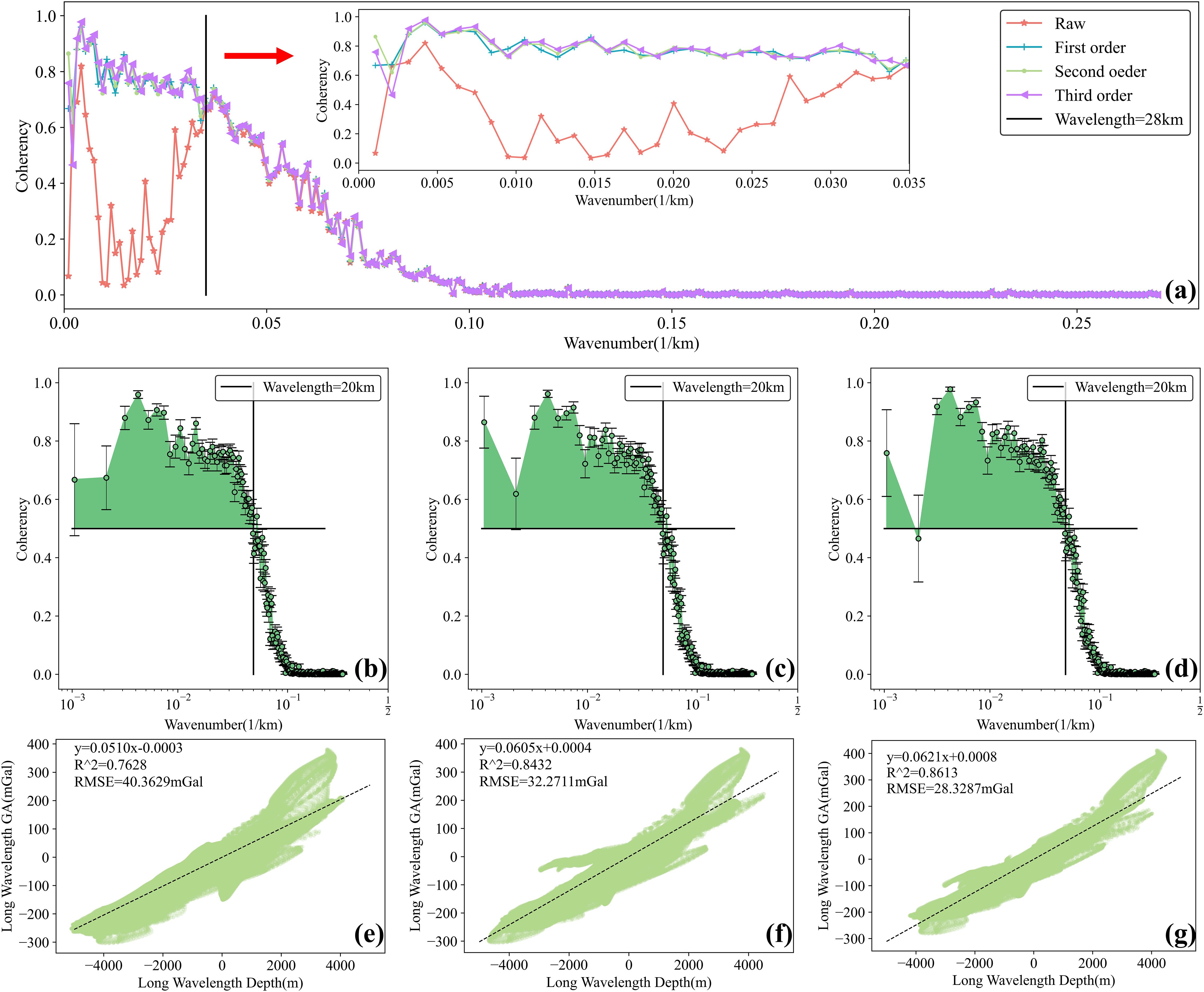
Figure 3. Comparison of the first to third-order detrending results for gravity anomaly and depth data (SIO v25.1). (A) Coherence between gravity anomaly and depth data after first to third-order detrending; (B) Coherence between gravity anomaly and depth data after first to third-order detrending for wavelengths greater than 28 km; (C–E) Coherence between gravity anomaly and depth data after first, second, and third-order detrending, respectively; (F–H) Linear regression between long-wavelength depth and long-wavelength gravity anomaly (wavelengths greater than 20 km) after first, second, and third-order detrending, respectively.

Figure 4

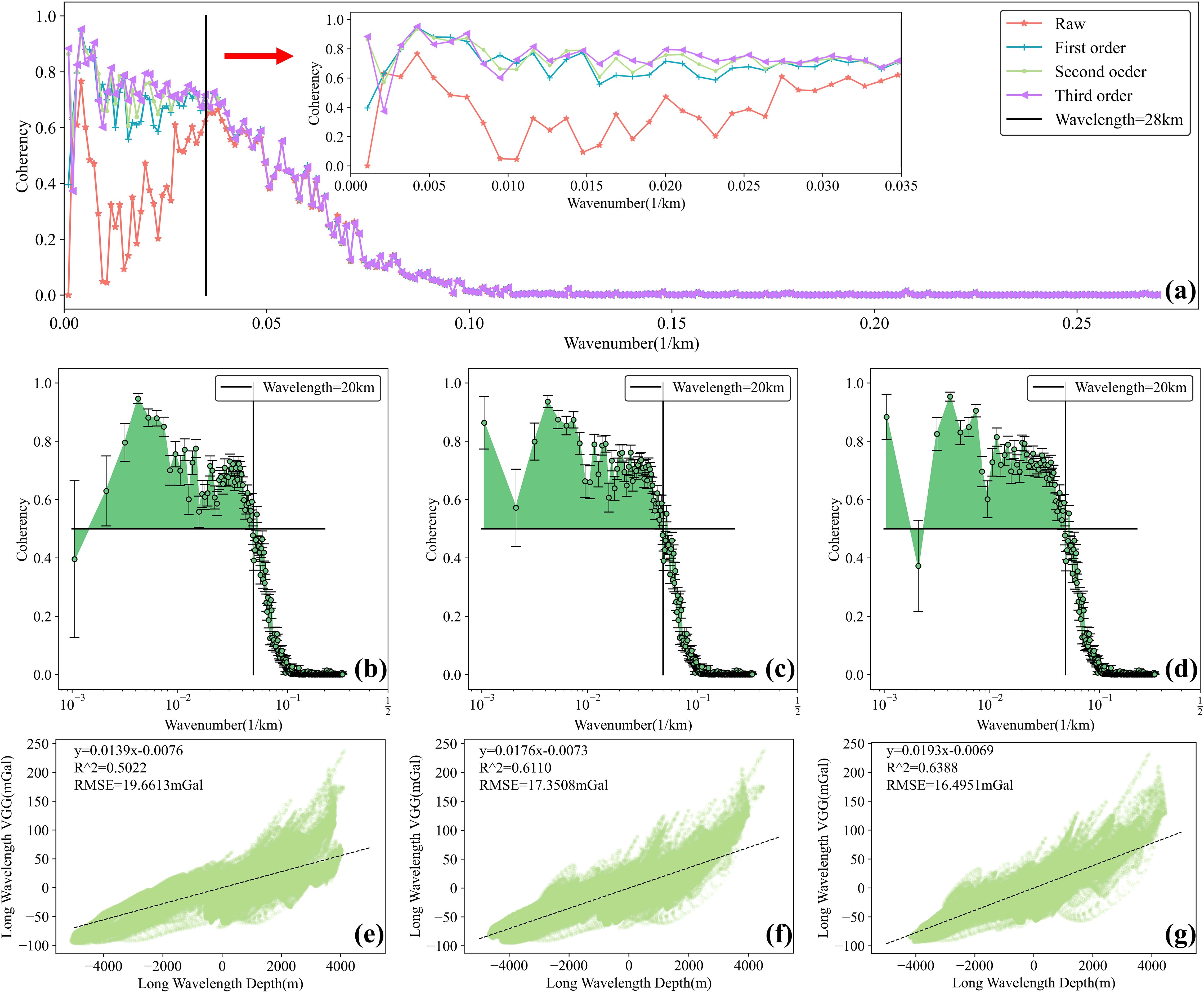
Figure 4. Comparison of the first to third-order detrending results for vertical gravity gradient anomaly and depth data (SIO v25.1). (A) Coherence between vertical gravity gradient anomaly and depth data after first to third-order detrending; (B) Coherence between vertical gravity gradient anomaly and depth data after first to third-order detrending for wavelengths greater than 28 km; (C–E) Coherence between vertical gravity gradient anomaly and depth data after first, second, and third-order detrending, respectively; (F–H) Linear regression between long-wavelength depth and long-wavelength vertical gravity gradient anomaly (wavelengths greater than 20 km) after first, second, and third-order detrending, respectively.

Figures 3B–D, 4B–D show the coherence of the gravity and depth data after first to third-order detrending. To select the most effective detrending method, linear regression was applied to the bands with coherence greater than 0.5 for each detrending, corresponding to long-wave components with wavelengths greater than 20 km. The goodness of fit (R²) and root mean square error (RMSE) were used to evaluate the linear regression results. An R² value close to 1 indicates the linear regression is effective, and an RMSE close to zero is optimal.

Figures 3E–G, 4E–G show the linear regression results after first to third-order detrending. The results indicate that third-order detrending produced the best linear regression outcomes. The R² for the linear regression between long-wavelength depth and GA data was 0.86, with an RMSE of 28.33mGal. The R² for the linear regression between long-wavelength depth and VGG data was 0.64, with an RMSE of 16.50mGal. Therefore, this paper selects third-order detrending. The scaling factor between long-wavelength depth and long-wavelength GA data is 0.06mGal/m, and the scaling factor between long-wavelength depth and long-wavelength VGG data is 0.02 E/m.

3.1.1.2 BPNN inversion results

Figure 5 shows the difference between the bathymetry model obtained from the BPNN (using the SIO bathymetry model as training data) and the single-beam data grid. Figure 6 shows the difference between the SIO bathymetry model and the single-beam data grid. The results indicate that the areas with more significant differences are concentrated in deep trench regions. Figure 7 demonstrates that when the SIO bathymetry model is used as the training data, the BPNN method achieves the optimal seafloor topography inversion at a spatial resolution of 15 arc-seconds. The RMSE is improved by 0.17 compared to the SIO model resampled to 15 arc-seconds.

Figure 5

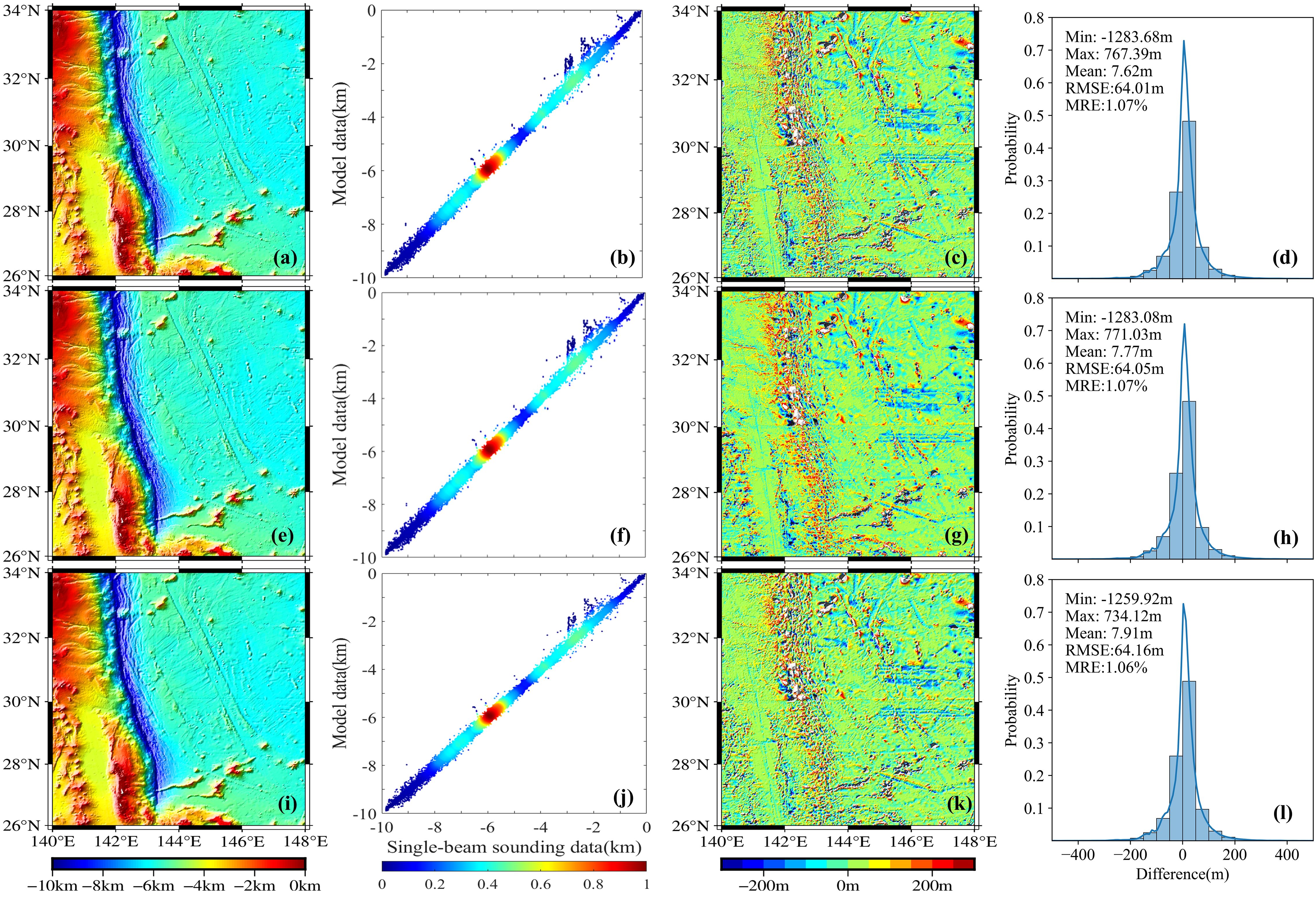
Figure 5. Differences between the bathymetry model from the BPNN (with 1 arc-minute SIO bathymetry model as the training data) and the single-beam data grid. (A, E, I) BPNN for 15 arc-seconds, 30 arc-seconds, and 1 arc-minute resolutions, respectively; (C, G, K) Spatial distribution of the differences between the BPNN at 15 arc-seconds, 30 arc-seconds, and 1 arc-minute resolutions and the corresponding single-beam data; (B, F, J) Scatter density plots comparing the BPNN at 15 arc-seconds, 30 arc-seconds, and 1 arc-minute resolutions with the corresponding single-beam data; (D, H, L) Distribution histograms of the differences between the BPNN at 15 arc-seconds, 30 arc-seconds, and 1 arc-minute resolutions and the corresponding single-beam data.

Figure 6

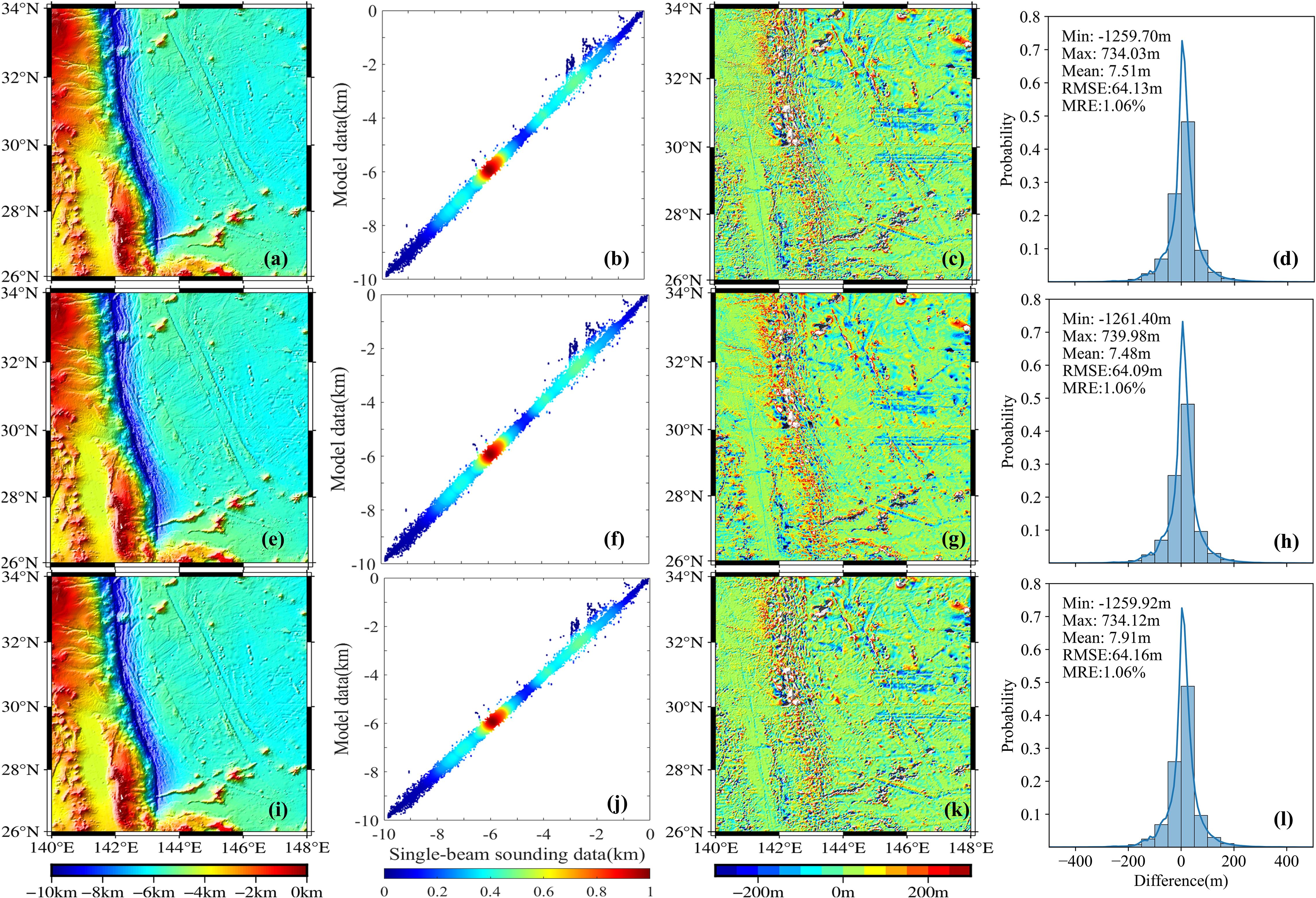
Figure 6. Differences between the inversion results using the 1 arc-minute SIO bathymetry model as the training data and the single-beam data grid. (A, E, I) SIO model at 15 arc-seconds, 30 arc-seconds, and 1 arc-minute resolutions, respectively; (C, G, K) Spatial distribution of the differences between the 15 arc-seconds, 30 arc-seconds, and 1 arc-minute SIO models and the corresponding single-beam data; (B, F, J) Scatter density plots comparing the 15 arc-seconds, 30 arc-seconds, and 1 arc-minute SIO models with the corresponding single-beam data; (D, H, L) Distribution histograms of the differences between the 15 arc-seconds, 30 arc-seconds, and 1 arc-minute SIO models and the corresponding single-beam data.

Figure 7

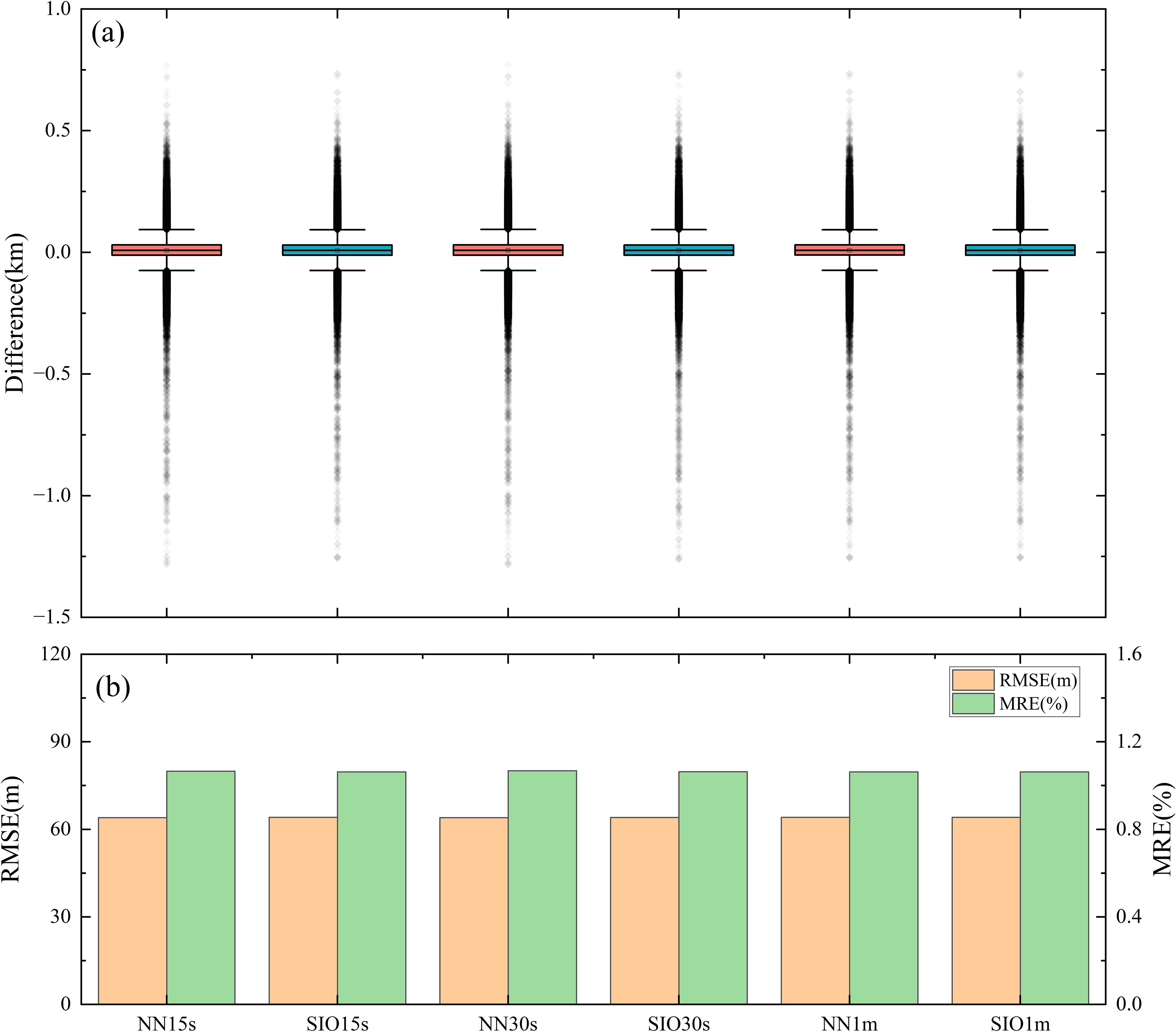
Figure 7. Differences between the bathymetry model (using the 1 arc-minute SIO model as the training data) and the single-beam data. (A) Box plot of the differences between the bathymetry model and the single-beam data; (B) Histogram of the differences between the bathymetry model and the single-beam data. “NN” denotes “BPNN”.

3.1.2 GEBCO 2023

Using GEBCO 2023 as the training data, coherence was similarly used to evaluate the effectiveness of various detrending operations. The relevant results can be found in Supplementary Material 2.1. Additionally, coherence analysis was conducted as with the GEBCO training data, and the results also indicated that third-order detrending achieved the best linear regression performance. Supplementary Figure 5 shows the differences between the BPNN bathymetry model, GEBCO model, and single-beam data grid. It can be observed that the areas with more significant differences are similarly concentrated in the deep trench regions. From Figure 8, it can be seen that when the resolution is 1 arc-minute, the BPNN method produces the best results, with the RMSE improved by 0.35% compared to the resampling results.

Figure 8

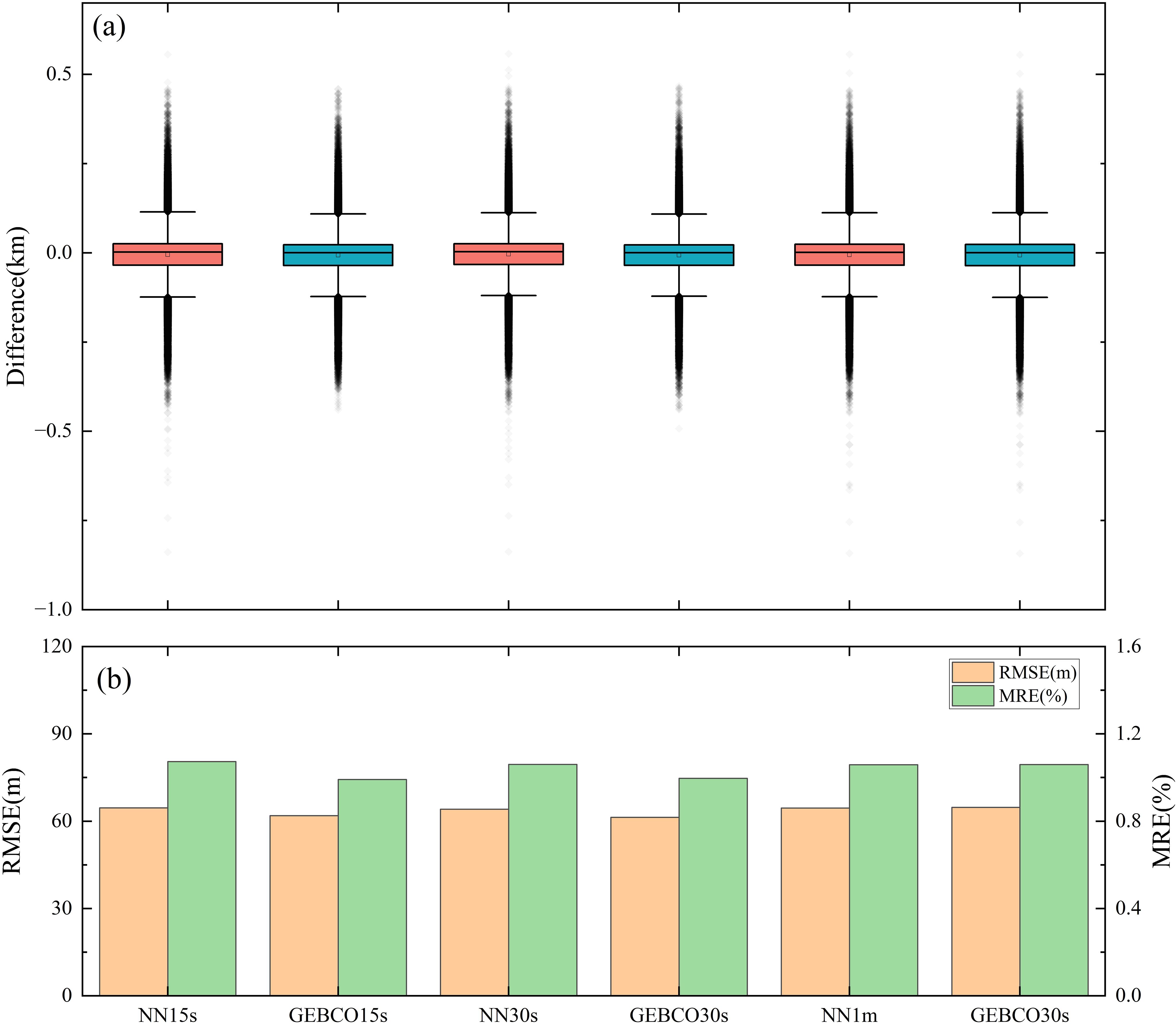
Figure 8. Differences between the bathymetry model (using the 1 arc-minute GEBCO model as the training data) and the single-beam data. (A) Box plot of the differences between the bathymetry model and the single-beam data; (B) Histogram of the differences between the bathymetry model and the single-beam data. “NN” denotes “BPNN”.

3.2 Seafloor topography prediction from the single-beam data

After data preprocessing, 220,276 single-beam bathymetry points were obtained, and 10,000 points were selected as checkpoints, with the remaining points used as input to construct the bathymetry model. Coherence was similarly used to evaluate the effectiveness of various detrending operations, with relevant results provided in Supplementary Material 2.2.

To assess the performance of the BPNN for seafloor topography inversion, the bathymetry model constructed using the BPNN method was compared with other bathymetry models.GGM is a commonly used high-precision bathymetry inversion method, while SIO and GEBCO are recognized as highly accurate global topography models. Both the GGM and BPNN bathymetry models were constructed using the same GA data. The GGM bathymetry model, based on the optimal density difference, as well as the SIO and GEBCO models, are shown in Supplementary Figure 6.

Supplementary Figure 7 shows the differences between the BPNN bathymetry model and other bathymetry models. The absolute difference statistics between the bathymetry model and the 10,000 checkpoints are presented in Figure 9. The results indicate that the BPNN model performs better. Specifically, when the spatial resolution is 15 arc-seconds, the RMS of the absolute difference between the BPNN bathymetry model and the checkpoints is 19.12m, which represents a 64.93% improvement over the GGM bathymetry model, a 70.29% improvement over the SIO model, and a 68.78% improvement over the GEBCO model. The mean relative error (MRE) of the absolute difference between the BPNN bathymetry model and the checkpoints is 0.18%, which is a 78.25% improvement over the GGM model, an 82.62% improvement over SIO, and an 81.74% improvement over GEBCO.

Figure 9

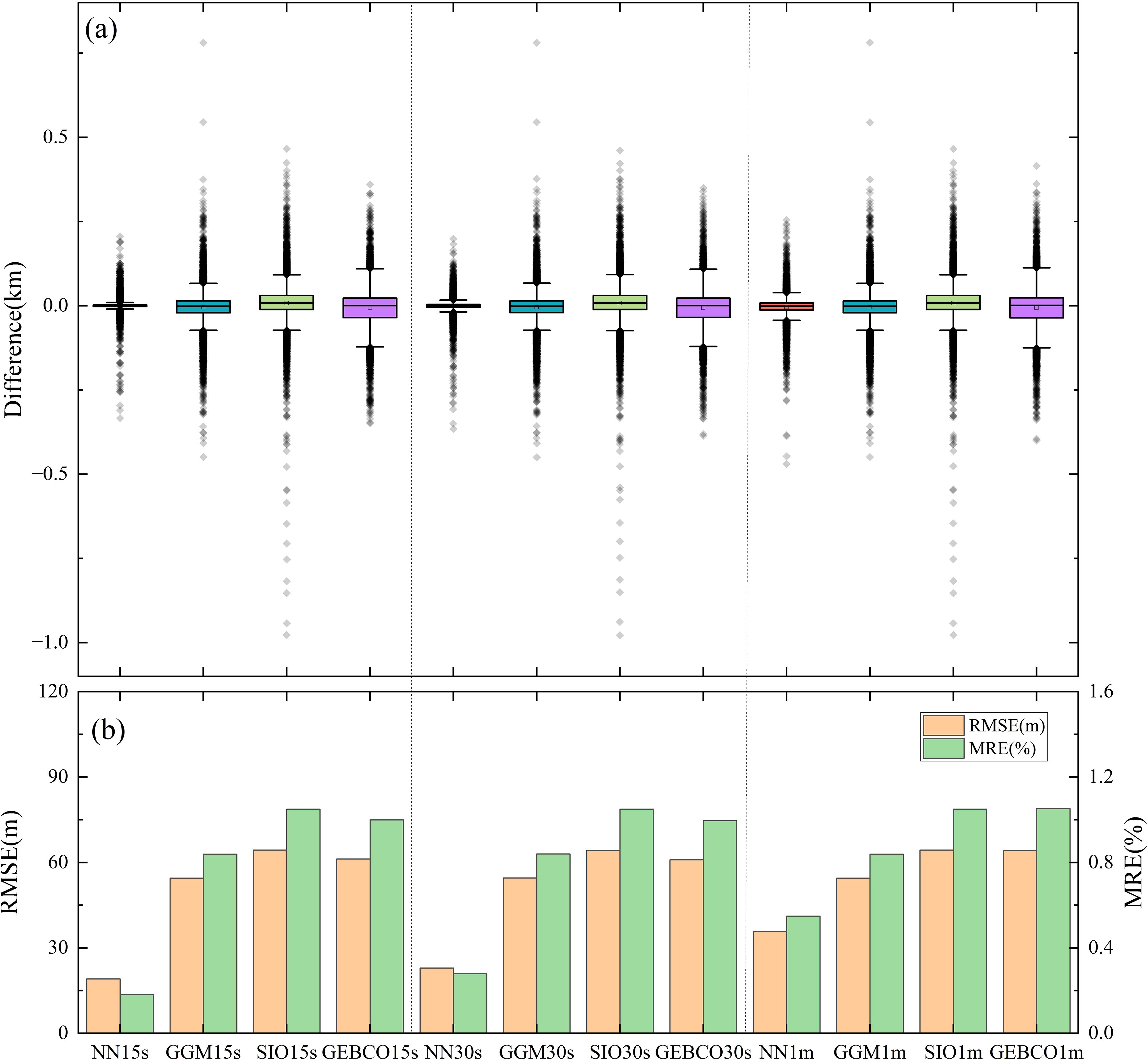
Figure 9. Differences between the bathymetry model (using single-beam data as the training data) and the checkpoints. (A) Box plot of the differences between the bathymetry model and the checkpoints; (B) Histogram of the differences between the bathymetry model and the checkpoints. “NN” denotes “BPNN”.

3.3 Effectiveness of gravity data fusion

This study designed three types of gravity data inputs for BPNN depth prediction to verify the effectiveness of gravity data fusion:1) Using both GA and VGG as input data; 2) Using only GA as input data; 3) Using only VGG as input data.

When single-beam data were used as training data, the inversion results for the three types of gravity data inputs are shown in Supplementary Figure 8. Figure 10 shows that when the resolution is 15 arc-seconds, the model using both GA and VGG data together has the smallest RMSE with the checkpoints, at 19.12m. This represents a 60.92% improvement compared to the model using only GA and a 61.13% improvement compared to the model using only VGG.

Figure 10

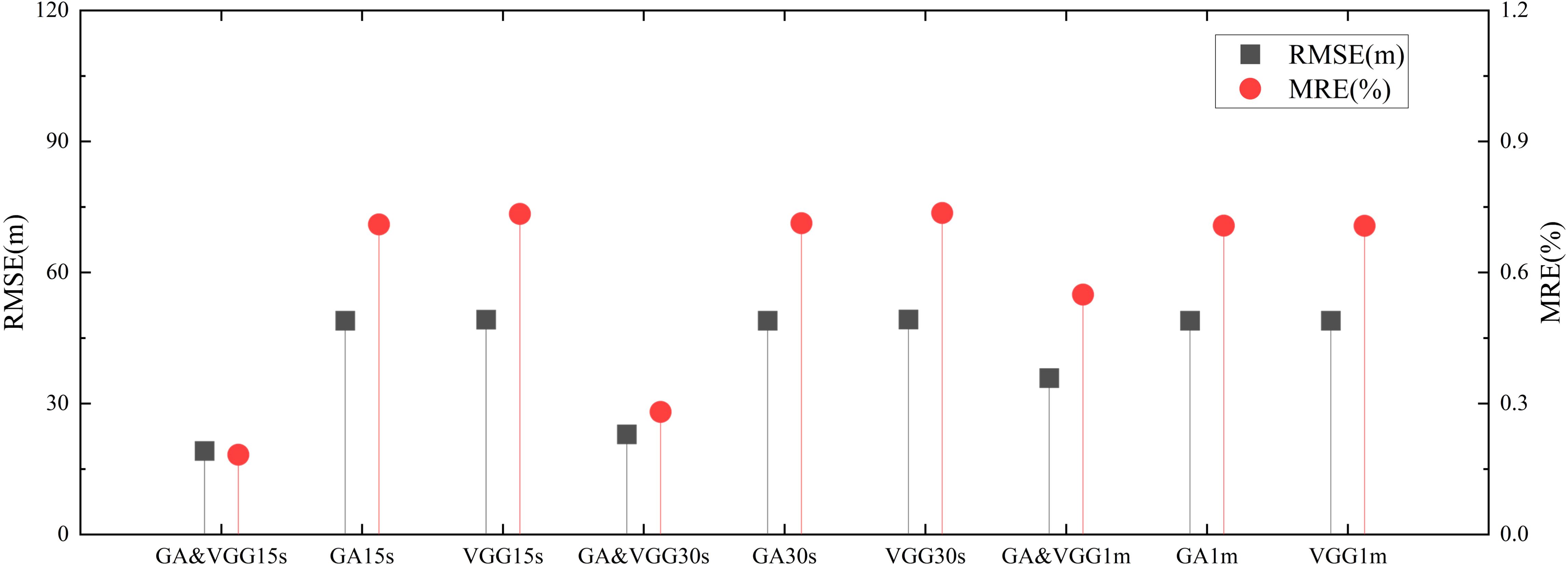
Figure 10. Differences between the seafloor topography results (using single-beam and gravity data fusion as input data) and the checkpoints.

3.4 Adaptability of the BPNN

By comparing the absolute differences between different bathymetry models and the checkpoints, the adaptability of the BPNN bathymetry model to various depths and topographies was verified. Seafloor topography is complex and diverse, so to validate whether the BPNN can adapt to complex terrain, three sub-regions were selected: a trench area (Area 1), a seamount area (Area 2), and a deep-sea plain area (Area 3) (as shown in Figure 1). These sub-regions were used to evaluate the performance of the BPNN in inverting seafloor topography.

The MRE between different bathymetry models and the checkpoints gradually decreases as depth increases, reaching a higher value at depths less than 1 km (Figure 11). In regions deeper than 5 km, the MRE stabilizes around 0.5%. At different depths, the MRE of the BPNN model is significantly lower than that of other bathymetry models, indicating that the BPNN is more effective at varying depths. From Figure 12, it can be observed that the RMS and MRE of the BPNN model are lower than those of other bathymetry models, and its inversion results are the best across all areas. The GGM underperforms in Area 2, the SIO models in Area 1, and the GEBCO models in Area 3, suggesting that the BPNN inversion method is universal and effective across various terrains.

Figure 11

Figure 11. MRE between the bathymetry model (using single-beam data as training data) and the checkpoints at different depths.

Figure 12

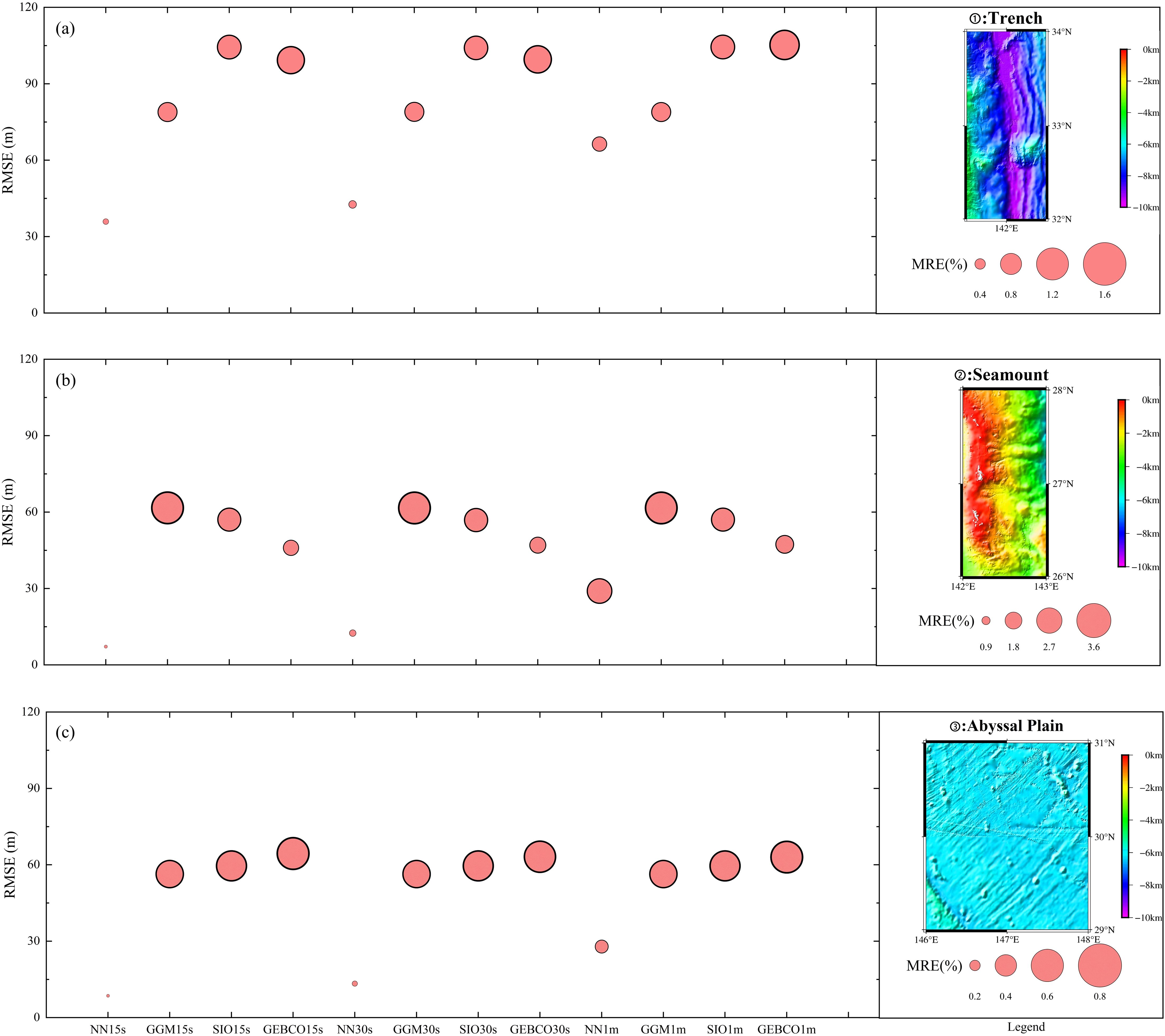
Figure 12. (A–C) Differences in the inversion bathymetry results (using single-beam data as the training data) for the three regions: ①Trench Area, ②Seamount Area, ③Abyssal Plain Area.

4 Conclusions

This study utilized gravity and gravity gradient data to predict seafloor topography in the Izu-Ogasawara Trench of the Western Pacific, using a dual-channel BPNN. Seafloor topography models and single-beam data were employed as training data. The performance of the BPNN for depth inversion was evaluated under different gravity data inputs, water depths, and terrain conditions. The main conclusions are as follows:

1. The BPNN method improves the accuracy and spatial resolution of depth inversion. When a 1 arc-minute model is used as training data, the BPNN method improves by 0.17% compared to the SIO model and by 0.35% compared to the GEBCO model. When single-beam data is used as training data, the BPNN method is closer to shipborne data than the GGM method, SIO model, and GEBCO model. Specifically, when the spatial resolution is 15 arc-seconds, the RMS of the absolute difference between the BPNN bathymetry model and the checkpoints is 19.12 meters, representing improvements of 64.93%, 70.29%, and 68.78% over the GGM, SIO, and GEBCO models, respectively. The MRE of the absolute difference between the BPNN bathymetry model and the checkpoints is 0.18%, representing improvements of 78.25%, 82.62%, and 81.74% over the GGM, SIO, and GEBCO models, respectively.

2. Fusion of gravity and gravity gradient data improves inversion accuracy. By comparing models using different gravity data, it was found that when the spatial resolution is 15 arc-seconds and single-beam data is used as training data, the model using both GA and VGG data had the smallest RMSE with the checkpoints, at 19.12 meters. This represents a 60.92% improvement compared to the model using only GA and a 61.13% improvement compared to the model using only VGG.

3. The BPNN method can adapt to different depths and terrain conditions. By comparing the BPNN bathymetry model with other bathymetry models at different depths, it was found that the MRE between the BPNN model and the checkpoint data is significantly lower at all depths than the other models, stabilizing around 0.5%. In different terrain conditions, the BPNN model consistently performed better than other models. When the spatial resolution is 15 arc-seconds and single-beam data is used as the target variable input, the BPNN method achieved an RMS error of 7.18 meters in Area 2, representing improvements of 88.36%, 87.42%, and 84.39% compared to the GGM, SIO, and GEBCO bathymetry models, respectively.

This study demonstrates the potential of BPNN in enhancing the resolution of seafloor topography. Using gravity data with a resolution of 1 arc-minute as input, increasing the resolution of the training data significantly improves the accuracy of the results. Although this study verified the accuracy of using the BPNN for seafloor topography inversion with different input data and target variables, it was only conducted in the Izu-Ogasawara Trench of the Western Pacific. In future research, this deep learning method will be applied to invert seafloor topography in different ocean regions and even globally. Furthermore, this study focused solely on the BPNN method, which does not account for specific physical mechanisms. Future work will further explore BPNN methods based on physical mechanisms for the global seafloor topography prediction.

Data availability statement

The datasets presented in this study can be found in online repositories. The names of the repository/repositories and accession number(s) can be found below: https://doi.org/10.7910/DVN/LKE2XY.

Author contributions

JL: Conceptualization, Data curation, Formal analysis, Writing – original draft, Writing – review & editing. NC: Conceptualization, Methodology, Visualization, Writing – review & editing. HL: Conceptualization, Methodology, Writing – review & editing. GC: Formal analysis, Writing – review & editing. SB: Supervision, Writing – review & editing. ZW: Visualization, Writing – review & editing. AM: Formal analysis, Writing – review & editing.

Funding

The author(s) declare financial support was received for the research, authorship, and/or publication of this article. This study is supported by the National Science Foundation for Outstanding Young Scholars (No.42122025), NSFC (China) under Grants 42274115, 42430101, and 42274003, the Opening Fund of Key Laboratory of Geological Survey and Evaluation of Ministry of Education (Grant No. GLAB2023ZR04) and the Fundamental Research Funds for the Central Universities.

Acknowledgments

The authors thank the following data providers for making the data available: shipborne single-beam data from NCEI, Gravity Anomalies and Vertical Gravity Gradient Anomalies data, Bathymetry model SIO v25.1 from SIO, and Bathymetry model GEBCO 2023 from GEBCO.

Conflict of interest

The authors declare that the research was conducted in the absence of any commercial or financial relationships that could be construed as a potential conflict of interest.

Publisher’s note

All claims expressed in this article are solely those of the authors and do not necessarily represent those of their affiliated organizations, or those of the publisher, the editors and the reviewers. Any product that may be evaluated in this article, or claim that may be made by its manufacturer, is not guaranteed or endorsed by the publisher.

Supplementary material

The Supplementary Material for this article can be found online at: https://www.frontiersin.org/articles/10.3389/fmars.2024.1520401/full#supplementary-material

References

Calmant S. (1994). Seamount topography by least-squares inversion of altimetric geoid heights and shipborne profiles of bathymetry and/or gravity anomalies. Geophysical J. Int. 119, 428–452. doi: 10.1111/j.1365-246X.1994.tb00133.x

Crossref Full Text | Google Scholar

Fan D., Li S. S., Li X. X., Yang J. J., Wan X. Y. (2021). Seafloor topography estimation from gravity anomaly and vertical gravity gradient using nonlinear iterative least square method. Remote Sens. 13, 19. doi: 10.3390/rs13010064

Crossref Full Text | Google Scholar

Harper H., Sandwell D. T. (2024). Global predicted bathymetry using neural networks. Earth Space Sci. 11, 9. doi: 10.1029/2023EA003199

Crossref Full Text | Google Scholar

Hsiao Y. S., Kim J. W., Kim K. B., Lee B. Y., Hwang C. (2011). Bathymetry estimation using the gravity-geologic method: an investigation of density contrast predicted by the downward continuation method. Terrestrial Atmospheric Oceanic Sci. 22, 347–358. doi: 10.3319/TAO.2010.10.13.01(Oc)

Crossref Full Text | Google Scholar

Jena B., Kurian P. J., Swain D., Tyagi A., Ravindra R. (2012). Prediction of bathymetry from satellite altimeter based gravity in the Arabian Sea: Mapping of two unnamed deep seamounts. Int. J. Appl. Earth Observation Geoinformation 16, 1–4. doi: 10.1016/j.jag.2011.11.008

Crossref Full Text | Google Scholar

Kim K. B., Hsiao Y. S., Kim J. W., Lee B. Y., Kwon Y. K., Kim C. H. (2010). Bathymetry enhancement by altimetry-derived gravity anomalies in the East Sea (Sea of Japan). Mar. Geophysical Res. 31, 285–298. doi: 10.1007/s11001-010-9110-0

Crossref Full Text | Google Scholar

Lehodey P., Grandperrin R. (1996). Swath mapping of the seafloor and its application to deep-bottom fisheries in New Caledonia. Mar. Geophysical Res. 18, 449–458. doi: 10.1007/BF00286089

Crossref Full Text | Google Scholar

Noei E. G., Hasanlou M., Sharifi M. A. (2018). Investigating effects of seafloor topography on sea surface currents in the Caspian Sea and northern Indian Ocean. J. Indian Soc. Remote Sens. 46, 2093–2106. doi: 10.1007/s12524-018-0886-8

Crossref Full Text | Google Scholar

Parker R. L. (1973). The rapid calculation of potential anomalies. Geophysical J. R. Astronomical Soc. 31, 447–455. doi: 10.1111/j.1365-246X.1973.tb06513.x

Crossref Full Text | Google Scholar

Schorghofer N. (2010). Expressions for tidal conversion at seafloor topography using physical space integrals. Fluid Dynamics Res. 42, 24. doi: 10.1088/0169-5983/42/6/065503

Crossref Full Text | Google Scholar

Smith W. H. F. (2004). Introduction to this special issue on bathymetry from space. Oceanography 17, 6–7. doi: 10.5670/oceanog.2004.62

Crossref Full Text | Google Scholar

Smith W. H. F., Sandwell D. T. (1994). Bathymetric prediction from dense satellite altimetry and sparse shipboard bathymetry. J. Geophysical Research-Solid Earth 99, 21803–21824. doi: 10.1029/94JB00988

Crossref Full Text | Google Scholar

Smith W. H. F., Sandwell D. T. (1997). Global sea floor topography from satellite altimetry and ship depth soundings. Science 277, 1956–1962. doi: 10.1126/science.277.5334.1956

Crossref Full Text | Google Scholar

Sun H. Y., Feng Y. K., Fu Y. G., Sun W. K., Peng C., Zhou X. H., et al. (2022). Bathymetric prediction using multisource gravity data derived from a parallel linked BP neural network. J. Geophysical Research-Solid Earth 127, 13. doi: 10.1029/2022JB024428

Crossref Full Text | Google Scholar

Sutton T. T., Porteiro F. M., Heino M., Byrkjedal I., Langhelle G., Anderson C. I. H., et al. (2008). Vertical structure, biomass and topographic association of deep-pelagic fishes in relation to a mid-ocean ridge system. Deep Sea Res. Part II: Topical Stud. Oceanography 55, 161–184. doi: 10.1016/j.dsr2.2007.09.013

Crossref Full Text | Google Scholar

Tscherning C. (1994). Geoid Determination by Least-square Collocation Using GRAVSOFT. International School for Determination and Use of the Geoid: Lecture notes; International Geoid Service, DIIAR, Politecnico di Milano: Milan, Italy.

Google Scholar

Wan X. Y., Ran J. J., Jin S. G. (2019). Sensitivity analysis of gravity anomalies and vertical gravity gradient data for bathymetry inversion. Mar. Geophysical Res. 40, 87–96. doi: 10.1007/s11001-018-9361-8

Crossref Full Text | Google Scholar

Wang Y. M. (2000). Predicting bathymetry from the earth's gravity gradient anomalies. Mar. Geodesy 23, 251–258. doi: 10.1080/01490410050210508

Crossref Full Text | Google Scholar

Watts A. B. (1978). An analysis of isostasy in the world's oceans 1. Hawaiian-Emperor Seamount Chain. J. Geophysical Research: Solid Earth 83, 5989–6004. doi: 10.1029/JB083iB12p05989

Crossref Full Text | Google Scholar

Wegner S. A., Campbell K. J. (2014). Drilling hazard assessment for hydrate bearing sediments including drilling through the bottom-simulating reflectors. Mar. Petroleum Geology 58, 382–405. doi: 10.1016/j.marpetgeo.2014.08.007

Crossref Full Text | Google Scholar

Xiang X. S., Wan X. Y., Zhang R. N., Li Y., Sui X. H., Wang W. B. (2017). Bathymetry inversion with the gravity-geologic method: A study of long-wavelength gravity modeling based on adaptive mesh. Mar. Geodesy 40, 329–340. doi: 10.1080/01490419.2017.1335257

Crossref Full Text | Google Scholar

Yang L., Liu M., Liu N., Guo J. Y., Lin L. A., Zhang Y. Y., et al. (2023). Recovering bathymetry from satellite altimetry-derived gravity by fully connected deep neural network. IEEE Geosci. Remote Sens. Lett. 20, 5. doi: 10.1109/LGRS.2023.3302992

Crossref Full Text | Google Scholar

Zhang F., Jin S., El Rhadiouini C. (2024). Seafloor topography of Huangyan seamount chain based on GA-BP algorithm from ship survey and gravity anomaly data. Mar. Geodesy 47, 269–288. doi: 10.1080/01490419.2024.2347877

Crossref Full Text | Google Scholar