Global surface eddy mixing ellipses: spatio-temporal variability and machine learning prediction

Mesoscale eddy mixing significantly influences ocean circulation and climate system. Coarse-resolution climate models are sensitive to the specification of eddy diffusivity tensor. Mixing ellipses, derived from eddy diffusivity tensor, illustrate mixing geometry, i.e., the magnitude, anisotropy, and dominant direction of eddy mixing. Using satellite altimetry data and the Lagrangian single-particle method, we estimate eddy mixing ellipses across the global surface ocean, revealing substantial spatio-temporal variability. Notably, large mixing ellipses predominantly occur in eddy-rich and energetic ocean regions. We also assessed the predictability of global mixing ellipses using machine learning algorithms, including Spatial Transformer Networks (STN), Convolutional Neural Network (CNN) and Random Forest (RF), with mean-flow and eddy- properties as features. All three models effectively represent and predict spatiotemporal variations, with the STN model, which incorporates an adaptive spatial attention mechanism, outperforming RF and CNN models in predicting mixing anisotropy. Feature importance rankings indicate that eddy velocity magnitude and eddy size are the most significant factors in predicting the major axis and anisotropy. Furthermore, training the models with a 2-year temporal duration, aligned with the El Niño Southern Oscillation (ENSO) timescale, improved predictions in the northern equatorial central Pacific region compared to models trained with a 12-year duration. This resulted in a spatially averaged correlation increase of over 0.5 for predicting the minor axis and anisotropy, along with a reduction of more than 0.15 in the Normalized Root Mean Square Error. These findings highlight the considerable potential of machine learning algorithms in predicting mixing ellipses and parameterizing eddy mixing processes within climate models.

1 Introduction

Mesoscale eddies play a critical role in large-scale ocean circulation and climate system by stirring and mixing crucial tracers. However, due to computational constraints, coarse-resolution climate models struggle to fully resolve subgrid eddy mixing processes, necessitating effective parameterization of eddy diffusivity. Climate model results are sensitive to both the magnitude and spatio-temporal structure of eddy diffusivity (Simmons et al., 2004; Danabasoglu and Marshall, 2007; Liu et al., 2012; Busecke and Abernathey, 2019). For example, Holmes et al. (2022) found that incorporating horizontal variations in eddy diffusivity, rather than constant values or scaling with grid resolution, along with the effects of mixing suppression by mean flows improves model agreement with observations of overturning circulation and tracer transport. While most studies have focused on estimating global cross-stream and along-stream components of the eddy diffusivity tensor (Ferrari and Nikurashin, 2010; Zhang et al., 2023c), shear dispersion often results in ubiquitous anisotropic eddy-induced transport (Berloff et al., 2002; Bachman et al., 2020; Haigh et al., 2021). Consequently, employing the full diffusivity tensor, rather than scalar coefficients, provides a more accurate representation of eddy mixing transport. Bovenschen (2021) demonstrated that incorporating anisotropic diffusivities enhances model performance, particularly in tidal regions and areas with strong shear gradients. Unlike previous studies that primarily emphasize cross-stream diffusivity, we focus on characterizing and predicting mixing ellipses, which depict the magnitude, anisotropy, and orientation of the eddy diffusivity tensor.

Although eddy mixing ellipses have been studied in idealized scenarios, their realistic depiction on a global scale, which is essential for developing plausible parameterizations, remains limited. Most existing research has focused on specific regions or used idealized models (Kamenkovich et al., 2009; Abernathey et al., 2013; Kamenkovich et al., 2015; Wolfram et al., 2015; Haigh et al., 2021; Wei and Wang, 2021; Zhang and Wolfe, 2022). For instance, Chen and Waterman (2017) applied a highly simplified barotropic quasi-geostrophic model to study mixing ellipses in a western boundary current jet. Their findings revealed that properties of mixing ellipses vary with flow regime, such that regions dominated by wave radiation exhibiting pronounced anisotropy, while mixing ellipses inside recirculation zones are nearly isotropic. Bachman et al. (2020) estimated mixing ellipses and anisotropy through a multiple-tracer inversion method and idealized mesoscale eddy-resolving simulations. Their results showed that, in regions of high kinetic energy, the major eigenvector of ellipses aligns primarily along the along-stream direction. However, such idealized models often simplify dynamics, assume homogeneous conditions, and impose artificial boundaries, limiting their ability to simulate the full complexity and variability of real ocean systems.

While machine learning algorithms have shown promise in predicting cross-stream eddy diffusivities (Guan et al., 2022; Zhang et al., 2023c), their application to the prediction of mixing ellipses remains largely unexplored. Recent advancements in machine learning techniques have yielded significant progress in various fields, including ship classification and detection (e.g., Guan et al., 2023; Zhang et al., 2023a; Gao et al., 2023b, e). Inspired by these advancements, we aim to apply a novel approach to predict eddy diffusivities, a crucial step toward the design and development of eddy diffusivity tensor parameterizations for climate models. Guan et al. (2022) applied Random Forest (RF) and Convolutional Neural Network (CNN) models to predict the spatial distribution of cross-stream eddy diffusivities in the Kuroshio Extension. Additionally, RF model has been used to predict regionally averaged time series of cross-stream eddy diffusivities across eight surface ocean regions (Zhang et al., 2023c). However, besides these traditional methodologies, we introduce Spatial Transformer Networks (STN) as a novel machine learning approach for predicting mixing ellipses. STN can enhance network performance by adaptively learning spatial transformations (e.g., scaling, cropping, rotations, and non-grid deformations) without manual parameter specification. We systematically evaluate the performance of STN, CNN, and RF models in predicting three key attributes of eddy mixing ellipses: major axis, minor axis and anisotropy.

We chose satellite altimeter data for both estimating and predicting global mixing ellipses due to its advantages over other observational ways. Traditional techniques, such as drift buoys, fixed-point, and shipborne observations, are often constrained by oceanic environmental conditions and limited spatial coverage. In contrast, radar altimeters on microwave remote sensing satellites provide consistent, all-weather, and all-day global observations, making them ideal for studying global mesoscale ocean phenomena. By analyzing the pulse echo signal characteristics directly beneath the satellite, radar altimeters precisely measure sea surface height, backscatter coefficients, and current velocities. While Synthetic Aperture Radar (SAR), another active microwave remote sensor, offers high-resolution observations by measuring microwave backscattered signals and phases (Zhang et al., 2024a), its global application remains limited. Advanced SAR techniques, such as dual-polarized, full polarimetric (Raney, 2016), compact polarimetric SAR (Zhang et al., 2022), polarimetric autocorrelation matrix methods (Zhang et al., 2024b), and onboard multisatellite information fusion (Gao et al., 2023c), have shown promise in enhancing ocean current monitoring, but comprehensive global analyses using SAR are still unrealized.

In summary, this study aims to estimate the spatio-temporal variability of global surface eddy mixing ellipses using Lagrangian single-particle method and to predict the features of mixing-ellipse attributes using machine learning models. This paper is organized as follows. Section 2 describes the dataset, including satellite altimetry data and Lagrangian particle trajectories, and introduces the methods for estimating and predicting Lagrangian (“particle-based”) eddy mixing ellipses. Section 3 presents the description and spatio-temporal variability of surface eddy mixing ellipses, as well as the representative and predictive performance of machine learning methods. Section 4 discusses the feature importance ranking and equatorial analysis across three models. We summarize the findings and conclusions in section 5.

2 Data and method

2.1 Data

The surface geostrophic velocity field is obtained from the Archival Verification and Interpretation of Satellite Oceanographic (AVISO, http://www.aviso.altimetry.fr/) data set of the French National Space Agency. We utilize the AVISO product spanning from 1994/01 to 2017/12, with a daily temporal resolution and a spatial resolution of 0.25° × 0.25°. The dataset employs the empirically validated “equatorial–geostrophic” approximation by Lagerloef et al. (1999) to compute velocities within the equatorial region (between 5°N and 5°S). AVISO data has been applied in quite a few mixing studies (Abernathey and Marshall, 2013; Bates et al., 2014; Abernathey and Haller, 2018; Shao et al., 2023). For instance, Zhang et al. (2023c) estimated global cross-stream eddy diffusivity using the Lagrangian particle method and discussed its linkage with climate indices.

To estimate eddy mixing ellipses, we choose to use the trajectories of particles advected by the total geostrophic flow from satellite altimetry, whose total number is approximately 8 × 10⁵ per year (Figure 1). In brief, for each year (1994-2017), the numerical particles were deployed offline at a resolution of 0.2° × 0.2° globally. Then, these particles were advected through daily geostrophic velocities for one year using a fourth-order Runge-Kutta scheme, with a 20-minute time step. This particle trajectory dataset was originally developed by Zhang et al. (2023b, c) for cross-stream eddy mixing studies at the global ocean surface.

Figure 1

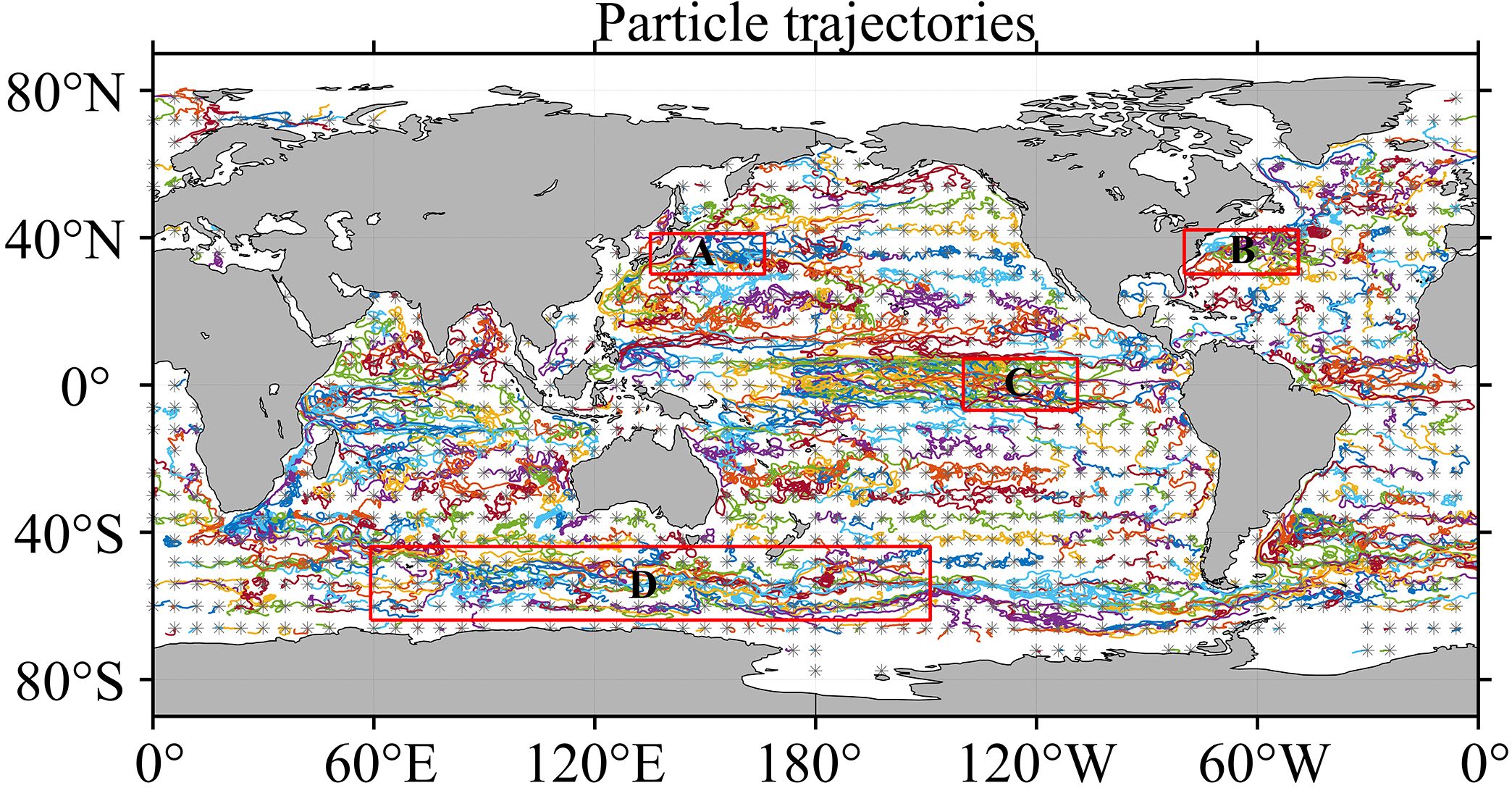
Figure 1. Sample particle trajectories released globally on 1 January 2010 and advected for one year. To make these trajectories visible, only trajectories from particles released at 6° intervals are shown here. Each gray dot marks the initial position of a trajectory. The areas of the red square marked (A–D) are denoted respectively as Kuroshio Extension (KE), Gulf Stream Extension (GSE), Equatorial Region and Antarctic Circumpolar Current (ACC).

2.2 Methods

2.2.1 Mixing ellipse estimation: Lagrangian single-particle method

Our study employs the Lagrangian single-particle method to estimate the mixing ellipses. Originally introduced by Davis (1987), this method has been proven to effectively estimate converged eddy diffusivities in scenarios involving inhomogeneous turbulence with mean flow (Griesel et al., 2014; Chen and Waterman, 2017; Liu et al., 2023). Following Chen and Waterman (2017), we set the initial positions of the pseudotrajectories at intervals of five days along each particle track. Each pseudotrajectory spans a duration of 115 days. Then we use an adaptive bin approach based on the K-means algorithm (Koszalka and LaCasce, 2010; Chen et al., 2014) to estimate the eddy diffusivity tensor. $k_{ij}^{\infty }$:

$\begin{array}{ll}{k}_{ij}^{\infty }(\mathbf{\text{x}})=\underset{\tau \to \infty }{\lim }{k}_{ij}(\mathbf{\text{x}},\tau )\approx \frac{{\int }_{{\tau }_1}^{{\tau }_2}{k}_{ij}(\mathbf{\text{x}},\tilde{\tau })d\tilde{\tau }}{{\tau }_2-{\tau }_1},& (1)\end{array}$

where

$\begin{array}{ll}{k}_{ij}(\mathbf{\text{x}},\tau )={\displaystyle {\int }_0^{\tau }d\tilde{\tau }\langle u_i^{{}^{\prime }}}(t_0|x,t_0)u_j^{{}^{\prime }}{(t_0+\tilde{\tau }|x,t_0)\rangle }_L.& (2)\end{array}$

Here $<·>$_L represents the ensemble average of all pseudotrajectories in the bin centered at x. The term $u_i^{{}^{\prime }}(t_0+\tilde{\tau }|x,t_0)$ denotes eddy velocity of particles at time $t_0+\tilde{\tau }$, passing through location x at t₀. Eddy velocity refers to the difference between the instantaneous Eulerian velocity $u_i(t_0+\tilde{\tau })$ and the annual-mean velocity $\overline{u}$. As the time τ increases, the component of eddy diffusivity tensor from Equation 2 gradually asymptotes to a constant value. The time τ at which the eddy diffusivity starts leveling off is termed as the equilibrium time τ = τ_eq. The converged value of eddy diffusivity from Equation 1 can be obtained simply by averaging k_ij (x,τ) over τ ∈ [τ₁,τ₂], where τ₁ = τ_eq − 15 (day) and τ₂ = τ_eq + 15 (day). For details of diagnosing τ_eq, see Chen and Waterman (2017).

The full eddy diffusivity tensor comprises both diffusive flux (symmetric components of $k_{ij}^{\infty }$) and skew flux (antisymmetric components of $k_{ij}^{\infty }$). The antisymmetric diffusivity tensor, equivalent to advection of tracers by non-divergent velocities, does not affect along-gradient fluxes (Vallis, 2006; Chen and Waterman, 2017; Kamenkovich et al., 2021). Therefore, our analysis focuses on the symmetric tensor S. Diffusion aligns with the eigenvectors’ orientation, forming an orthogonal basis called the principal axes of S. Each eigenvalue represents the diffusivity along its corresponding axis. The magnitude and direction of these principal axes form mixing ellipses (shown in Figure 2), which effectively characterize the strength, dominant direction and anisotropy of eddy mixing (Rypina et al., 2012; Chen and Waterman, 2017; Bachman et al., 2020).

Figure 2

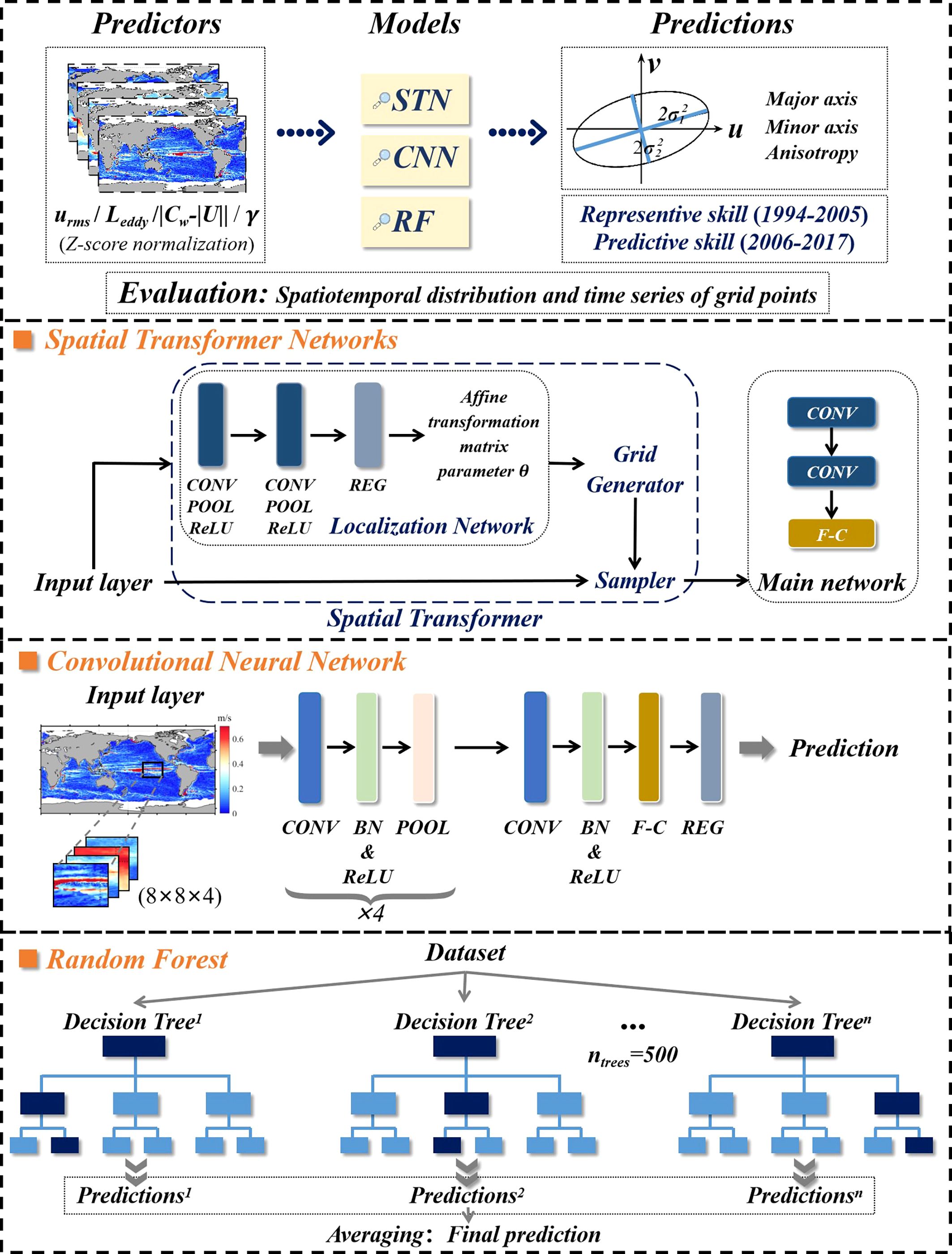
Figure 2. The flowchart and structure of the Spatial Transformer Networks (STN), Convolutional Neural Network (CNN) and Random Forest (RF) approaches for predicting three attributes (major axis, minor axis, and anisotropy) of mixing ellipses.

Following Chen and Waterman (2017), we calculated the component of the symmetric tensor S, defined as ${\sigma }_x^2, {\sigma }_y^2, {\sigma }_{xy}^2$ in Equation 3,

$\begin{array}{ll}{\sigma }_x^2=k_{xx},{\sigma }_y^2=k_{yy},{\sigma }_{xy}^2=\frac{k_{xx}+k_{yy}}{2}.& (3)\end{array}$

The lengths of the semimajor and semiminor axes, ${\sigma }_1^2, {\sigma }_2^2$, can be estimated from the eigenvalue of $S$, following

$\begin{array}{ll}{\sigma }_1^2=\frac{1}{2}\left[{\sigma }_x^2+{\sigma }_y^2+\sqrt{{({\sigma }_x^2-{\sigma }_y^2)}^2+4{({\sigma }_{xy}^2)}^2}\right],& (4)\end{array}$

$\begin{array}{ll}{\sigma }_2^2=({\sigma }_x^2+{\sigma }_y^2)-{\sigma }_1^2.& (5)\end{array}$

Mixing anisotropy measures the ellipse eccentricity. It can be diagnosed from

$\begin{array}{ll}Anisotropy=\frac{{\sigma }_2^2}{{\sigma }_1^2},& (6)\end{array}$

which ranges from zero to one. Zero (one) represents purely unidirectional (isotropic) ellipse. Therefore, small (large) value of Anisotropy corresponds to high (low) anisotropy of mixing ellipses. The ellipse orientation can be represented by θ, which denotes the anticlockwise angle of the semimajor axis relative to the positive x. The term tan(θ) satisfies,

$\begin{array}{ll}\text{tan }(\theta )=\frac{{\sigma }_1^2-{\sigma }_x^2}{{\sigma }_{xy}^2}.& (7)\end{array}$

2.2.2 Mixing ellipse prediction: machine learning method

Machine learning algorithms, known for their computational efficiency and ability to capture nonlinear relations between predictors and predictand, have been widely applied in oceanic and atmospheric predictions (Guan et al., 2022; Liu et al., 2023). For instance, Cao et al. (2024) introduced a deep learning model that significantly improves the retrieved of wave spectra and wave parameters. Similarly, Gao et al. (2024b) proposed a hybrid multiscale spatial-temporal model incorporating an error correlation map, leading to enhanced sea surface temperature predictions.

We apply three algorithms, STN, CNN, and RF, to predict mixing-ellipse attributes, each offering distinct advantages. The STN approach incorporates a spatial attention mechanism into a CNN framework, enabling robust image recognition under affine transformations such as scaling, rotation, and cropping. This self-supervised, end-to-end process has proven effective in other fields (e.g., Jaderberg et al., 2015; Mirmohammadsadeghi et al., 2017; Sinclair et al., 2022). The CNN approach extracts spatial features from input images through convolutional operations. CNN-based methods, including their variants, have demonstrated success in various applications, such as ship detection and classification (e.g., Guan et al., 2023; Gao et al., 2023a, d, 2024a). The RF approach can improve prediction accuracy through an ensemble of decision trees, each constructed by randomly selecting features at each split. This method is computationally efficient, resistant to overfitting, and has been successfully applied to predict across-stream eddy diffusivities (e.g., Ho, 1995; Su et al., 2018; Guan et al., 2022).

The architecture and implementation details of these three models are shown in Figure 2 and are described as follows:

● Model 1: STN integrates a Spatial Transformer module, which consists of three components: the Localization Network, the Grid Generator, and Differentiable Image Sampling. The Localization Network extracts spatial features and outputs a 6-dimensional vector representing the parameters of affine transformation matrix. The Grid Generator uses these parameters to compute transformed grid coordinates, while Differentiable Image Sampling applies bilinear interpolation to generate the transformed feature map. These transformed features are then processed by the main network, which includes two convolutional layers. The first layer is followed by Rectified Linear Unit (ReLU) activation and average pooling, while the second layer is followed by dropout, ReLU activation, and average pooling. The resulting feature map is then flattened and passed through a fully connected layer, followed by a dropout layer for regularization. The final fully connected layer produces the model’s output.

● Model 2: The CNN model’s architecture consists of 5 convolutional layers, 4 average pooling layers, 1 dropout layer (with a probability of 0.2), and 1 fully connected layer with an output size of 1. Batch normalization and ReLU activation function are applied after the first four convolutional layers to mitigate vanishing gradients and overfitting issues. Each convolutional layer uses a filter size of 2, with the number of neurons increasing from 8 to 32. The model is trained with a learning rate of 10^-4 for up to 70 epoches.

● Model 3: The RF model is computationally efficient and requires fewer parameters. The number of trees in the forest (n_trees) is set to 500, and the number of features in a random subset of each node (m_try) is set to 1.

The prediction procedure, as shown in Figure 2, involves four steps:

● Step 1: Dataset preparation. The original dataset includes the predictands and four predictors. The predictands are the major axis, minor axis and anisotropy of mixing ellipses, each with a spatial resolution of 1° × 1°. The predictors, chosen based on the Suppressed Mixing Length Theory (SMLT), are as follows: eddy size L_eddy, eddy velocity magnitude u_rms, the inverse of eddy decorrelation time scale γ, and eddy propagating speed relative to the mean flow $\left|C_w-\right|\mathbf{\text{U}}\Vert$ (see Section 2.2.3). The original dataset is divided into a training set and a test set to respectively assess the representative and predictive performance of the machine learning models. A Z-score normalization is conducted to rescale both predictors and predictands.

● Step 2: Model construction. In the RF model, the input variables are local grid points from the training set, with a resolution of 1°. For the STN and CNN models, the four predictors are extracted from overlapping subdomains, each covering an area of 2° × 2° and containing 8 × 8 grid points, with spatially averaged predictands serving as the counterpart output. The subdomain predictors are resampled at a higher resolution of 0.25°. Two dataset selection methods are used: (1) a “12-Year model”, where the training set comprises four predictors and the predictands spanning 1994-2005 and the test set covers the period 2006-2017, and (2) a “2-Year model”, where the training set consists of two years preceding the predicted year, and the test set corresponds to the predicted year (see Section 4.2).

● Step 3: Model representation and prediction. The models are trained and tested using the predictors from the training and test sets. For the 12-Year model, outputs include representative results (1994-2005) and predictive results (2006-2017) for the annual mean mixing-ellipse attributes across the global ocean. Here, the representative (predictive) skill refers to the goodness of fit to the training (test) set. For the 2-Year model, predictive skill is analyzed for each year from 2006 to 2017. This approach requires training 12 separate models, each corresponding to a different predicted year.

● Step 4: Performance evaluation. We evaluate the performance by calculating correlation coefficients and normalized root-mean-square error (NRMSE) between the representative (predictive) results (Y_ML) and their particle-based counterparts (Y_Particle) during the same period. NRMSE is defined as

$\begin{array}{ll}NRMSE=\frac{\sqrt{\frac{1}{N}{\Sigma }_1^N{(Y_{ML}-Y_{Particle})}^2}}{\sqrt{\frac{1}{N}{\Sigma }_1^N{(Y_{Particle})}^2}}.& (8)\end{array}$

2.2.3 Predictors from the suppressed mixing length theory

The predictors for our machine learning models (Figure 2) are the variables derived from SMLT, which has been formulated to express cross-stream eddy diffusivity (Ferrari and Nikurashin, 2010; Klocker and Abernathey, 2014). Recent studies have demonstrated that models employing these predictors (L_eddy, u_rms, γ, $\left|C_w-\right|\mathbf{\text{U}}\Vert$) can well represent the spatiotemporal variability of cross-stream eddy diffusivities, i.e., those in the cross-mean flow direction (Guan et al., 2022; Zhang et al., 2023c). Inspired by these findings, we utilize this predictor set to predict the eddy mixing-ellipse attributes.

The diagnosis of eddy and mean flow properties follows previous studies (e.g., Chen et al., 2014; Guan et al., 2022; Zhang et al., 2023c). Specifically, eddy size L_eddy is calculated by Equation 9, where the eddy wavenumber k_eddy is derived from the two-dimensional eddy kinetic energy (EKE) wavenumber spectrum. The spectrum is calculated over spatial regions spanning 3° in latitude and longitude. In Equation 10, k and l denote the zonal and meridional wavenumbers, respectively.

$\begin{array}{ll}{L}_{eddy}(x,y)=\frac{2\pi }{k_{eddy}(x,y)}& (9)\end{array}$

$\begin{array}{ll}{k}_{eddy}(x,y)=\frac{{\iint }^{}\sqrt{k^2+l^2}{S}_{EKE}(k,l)dkdl}{{\iint }^{}{S}_{EKE}(k.l)dkdl}& (10)\end{array}$

Eddy velocity magnitude $u_{rms}$ is defined as $\sqrt{u^{\prime 2}+v^{\prime 2}}$. Here, the zonal (meridional) eddy velocity $u^{\prime }(v^{\prime })$ is the deviations of the zonal (meridional) flow velocity u (v) from its annual-mean $\overline{u }(\overline{v})$. The inverse of eddy decorrelation timescale γ is computed using Equation 11, where a mixing efficiency of Γ = 0.35 is adopted based on previous studies (Chen et al., 2014; Klocker and Abernathey, 2014).

$\begin{array}{ll}\gamma (x,y)=\frac{u_{rms}(x,y)}{2\Gamma L_{eddy}(x,y)}& (11)\end{array}$

When estimating the eddy propagating speed relative to the mean flow $\left|C_w-\right|\mathbf{\text{U}}\Vert$, $\left|U\right|$ refers to the magnitude of the local annual-mean geostrophic flow vector U. Eddy phase speed C_w refers to eddy phase speed along the mean flow direction. As described by Guan et al. (2022) and Zhang et al. (2023c), C_w is extracted from the Hovmoller¨ diagram of sea level anomaly using the Radon transform method.

3 Results

3.1 Mixing ellipse estimation

3.1.1 Mixing ellipse description

Particle-based mixing ellipses have significant spatio-temporal variability at the global ocean surface. The mixing-ellipse area is especially large in eddy-rich and energetic ocean regions, such as the Kuroshio Extension (KE), Gulf Stream Extension (GSE), Antarctic Circumpolar Current (ACC) and equatorial zones, reflecting elevated eddy mixing. Figure 3 illustrates mixing ellipses for these key regions, with data from 2005 and 2008 for the KE to represent stable and unstable states (Qiu et al., 2014; Chen et al., 2017), and data from 2010 for other regions as an example. Intuitively, mixing ellipses in the KE region exhibit pronounced interannual variability, which is to a certain degree linked with the KE’s transition between stable (e.g. in 2005) and unstable (e.g. in 2008) states (Figures 3A, B).

Figure 3

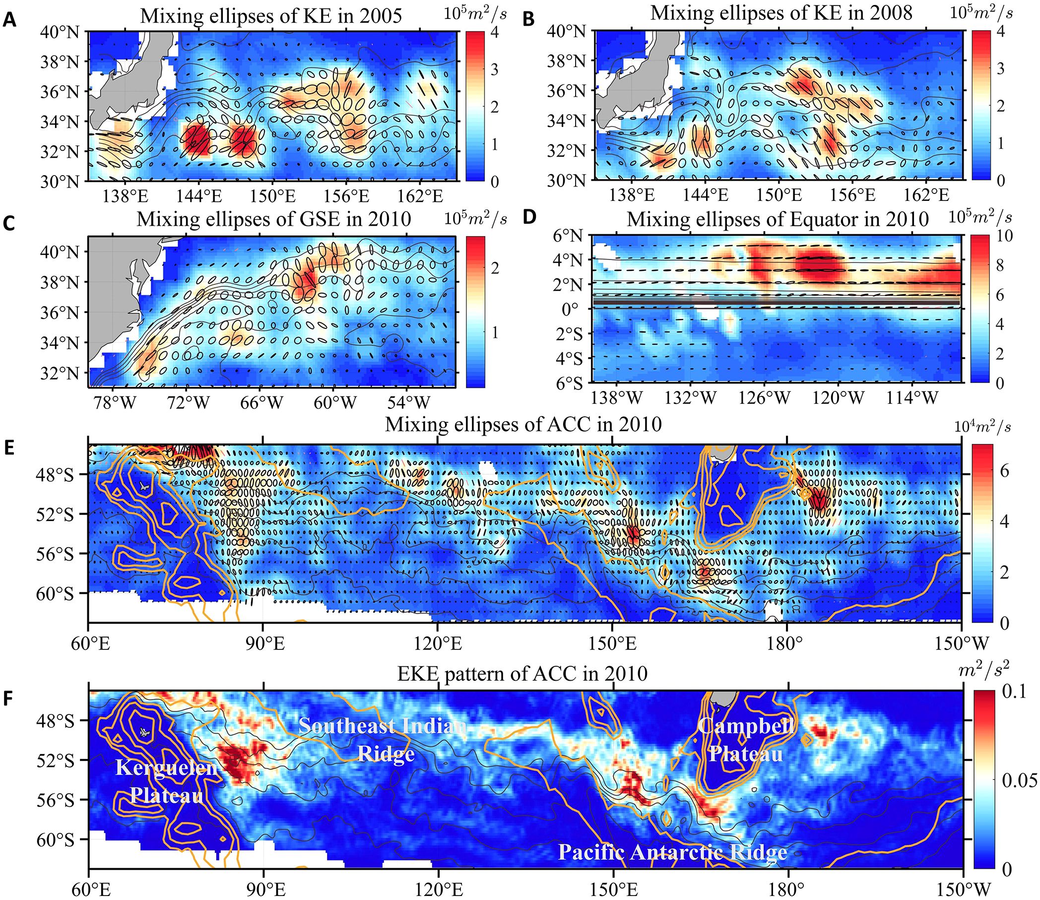
Figure 3. Mixing ellipses in four key regions: (A) KE in 2005, (B) KE in 2008, (C) GSE in 2010, (D) Equatorial Region in 2010, (E) ACC in 2010. (F) Spatial pattern of eddy kinetic energy of ACC in 2010 with the topography. Brown lines represent barotropic streamlines, as defined by ψ_g = gf⁻¹η, with η denoting annual-mean sea surface height, where g is the gravitational acceleration, and f denotes the Coriolis parameter. The colorbar shows the major axis length (m²/s), with axes of ellipses scaled down for visualization of their orientation relative to streamlines. The orange contours denote 500-, 1500-, 2500-, 3500-m bathymetry contours.

Mixing ellipses also have significant heterogeneity across these eddy-rich and energetic regions (Figures 3B-E). In the upstream of the KE and GSE jet, mixing ellipses tend to be elongated along the streamlines due to the suppression of mixing across the intense jet, leading to high anisotropy (Ferrari and Nikurashin, 2010; Chen et al., 2014; Wei and Wang, 2021). This feature is consistent with Nummelin et al. (2021), who found that strong mean flow elongates (squeezes) the mixing ellipses along (across) the mean flow direction. In contrast, in the downstream area, eddy motions dominate as the jet flow weakens and thus mixing across the jet is less suppressed and mixing ellipses are relatively circular. In the equatorial region, strong zonal jets tend to flatten eddy mixing ellipses, inducing strong mixing anisotropy.

In the ACC region, the spatial structure of mixing ellipses correlates tightly with topography and EKE patterns (Figures 3E, F). Consistent with literature (e.g., Sallée et al., 2011), in the downstream of large topography, such as the Kerguelen Plateau, the Southeast Indian Ridge, the Pacific Antarctic Ridge, and the Campbell Plateau, mixing suppression by the ACC jets locally breaks down and regional mixing becomes notably intensified. Here topographic steering forces the jet toward areas with decreased ambient potential vorticity gradient (Witter and Chelton, 1998) and generates local hotspots of mesoscale EKE downstream (Kong and Jansen, 2021), enhancing lateral mixing (Sallée et al., 2011; Foppert et al., 2017). The correlations between EKE and major/minor axis of mixing ellipses are both equal to 0.78 ± 0.1 at 95% confidence level. This high correlation value suggests that EKE plays a noticeable role in modulating eddy mixing intensity, consistent with the mixing length theory (Thompson and Garabato, 2014; Rosso et al., 2015; Guan et al., 2022).

3.1.2 Spatio-temporal structure of three attributes

The global variability of mixing ellipses can be effectively captured by their attributes, including major/minor axes and anisotropy. Consequently, to capture the spatial structure and quantify the temporal variability of mixing ellipses, we analyzed the climate-mean attributes and the standard deviation (STD) of the annual-mean attributes during two periods 1994-2005 (Supplementary Figure S1 in the supporting information) and 2006-2017 (Figure 4) respectively.

Figure 4

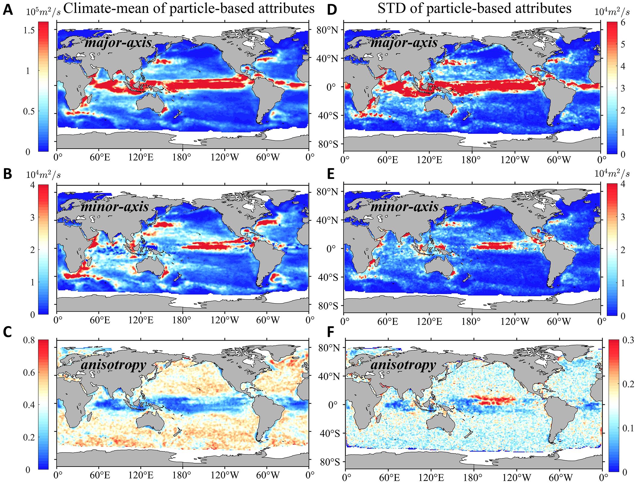
Figure 4. The climate-mean values of (A) major axis length (B) minor axis length (C) anisotropy and the standard deviation (STD) of (D) major axis length (E) minor axis length (F) anisotropy during 2006-2017 based on Lagrangian single-particle method.

The three climate-mean attributes exhibit highly uneven global spatial distributions (Supplementary Figures S1A-S1C, Figures 4A-C). Larger major (minor) axis length occurs in western boundary currents and their extensions, reaching up to 4.6 × 10⁵m²/s (1.1 × 10⁵m²/s). This phenomenon is also present throughout the entire equatorial zone for major axis. Additionally, elevated minor axis length can be observed in the northern equatorial central Pacific 110°W-170°W, 0°-15°N) during 2006-2017. In other quiescent regions (e.g., Southern Ocean etc.), the amplitudes of axes are relatively small and mixing tends to be isotropic.

The STD of the axes’ length shares a similar spatial distribution to their climate-mean values (Supplementary Figures S1D-S1E; Figures 4D, E). Mixing anisotropy exhibits high temporal variability exclusively in the northern equatorial central Pacific during 2006-2017 (Figure 4F). The normalized standard deviations (NSTD), defined as the ratio between the STD values and climate-mean values over the years 1994-2017, serve as a useful metric to measure temporal variability. The NSTD of the axes’ length exceeds 0.6 in high-latitude and equatorial regions (Figures 5A, B). The NSTD of mixing anisotropy has relatively small magnitudes in off-equatorial regions (Figure 5C). The probability density function (PDF) distribution of NSTD peaks at approximately 0.37 for major axis, 0.4 for minor axis and 0.31 for anisotropy (Figure 5D). The cumulative density function (CDF) reveals that NSTD of major (minor) axis exceeds 0.4 in 51% (69%) of the global ocean (Figure 5E). Our results illustrate that temporal variability is non-negligible in most regions of the global surface ocean.

Figure 5

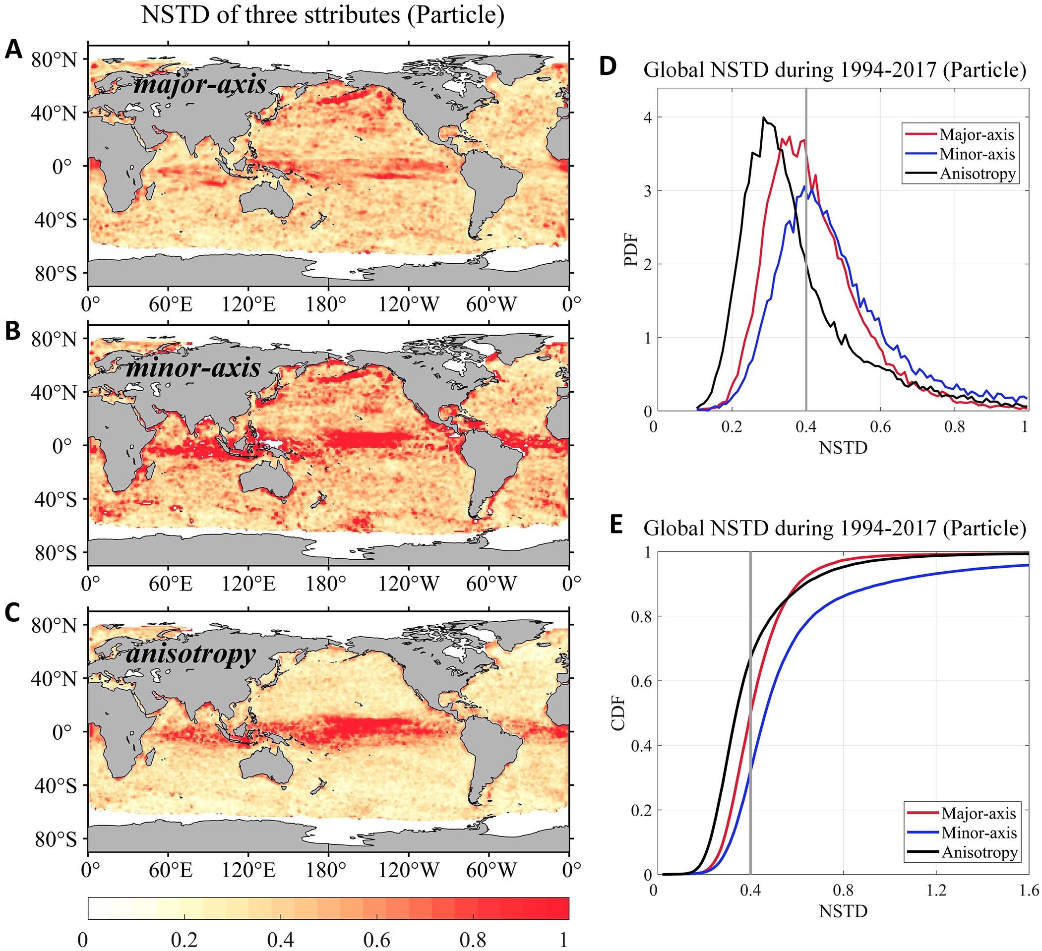
Figure 5. The normalized standard deviation (NSTD) of annual-mean particle-based attributes spanning from the year 1994-2017. Spatial pattern of NSTD of (A) major axis length (B) minor axis length (C) anisotropy. (D) Probability density function (PDF) and (E) the cumulative density function (CDF) of the NSTD from (A-C). The gray vertical lines in (D, E) indicate the NSTD value of 0.4.

3.2 Representation and prediction of mixing ellipse

This section assesses the performance of STN, CNN and RF models (“12-Year model”) in representing and predicting mixing ellipses, using factors derived from SMLT. Results predicted by the STN, CNN and RF models are referred to as “STN-based”, “CNN-based” and “RF-based”, respectively.

3.2.1 Representation skill

We compare the outputs of the machine learning models with particle-based attributes during 1994-2005 (Supplementary Figure S1) to evaluate the model’s representation skill. Among three models, RF model best represents both the magnitude and spatial structure of climate-mean values and STD values of mixing-ellipse attributes (Supplementary Figure S2). To quantify the representative skill, we estimated the global spatial correlation coefficients and NRMSE between particle-based attributes and those from each model over the 1994-2005 period. Correlation coefficients for RF model exceed 0.95 for all three attributes, with NRMSE values lower than 0.3 across all years. In comparison, both methods CNN and STN models are inferior to RF in representing mixing ellipses, with correlations (NRMSE) around 0.9 (0.4) for major axis, 0.8 (0.4-0.5) for minor axis and 0.7 (0.3) for mixing anisotropy.

To further assess the ability of models in representing the temporal variability, we calculated the temporal correlation coefficients and NRMSE between time series of particle-based attributes and those predicted by the models for each grid point from 1994 to 2005. Results indicate that the RF model performs well across the global surface ocean, with zonally averaged correlations for three mixing-ellipse attributes generally exceeding 0.9 cross latitudes (not shown). The CDF in Supplementary Figure S3 reveals that the correlation coefficients from RF model exceed 0.91 for major axis, 0.91 for minor axis, and 0.96 for anisotropy in 85% of the global ocean. The corresponding NRMSE values are below 0.24, 0.35 and 0.27, respectively. In contrast, the representative skills of CNN and STN is significantly inferior to those of RF.

3.2.2 Prediction skill

To evaluate the model’s prediction skills, we compared the outputs of machine learning models with particle-based attributes during 2006-2017 (Figure 4). The STN model accurately predicts the global climate-mean features of three attributes and the spatial distribution of the axes’ STD (Figure 6). But for mixing anisotropy, its temporal variability is underestimated. The predictive skill for minor axis and anisotropy in the northern equatorial central Pacific is weak, likely due to the influence of regional climate states. For example, different phases of El Niño Southern Oscillation (ENSO) may be averaged within the 12-Year model, resulting in reduced predictive accuracy. We found that using a 2- or 3-year data as training set, which better represents a single climate state, yields more accurate predictions, as discussed further in Section 4.2.

Figure 6

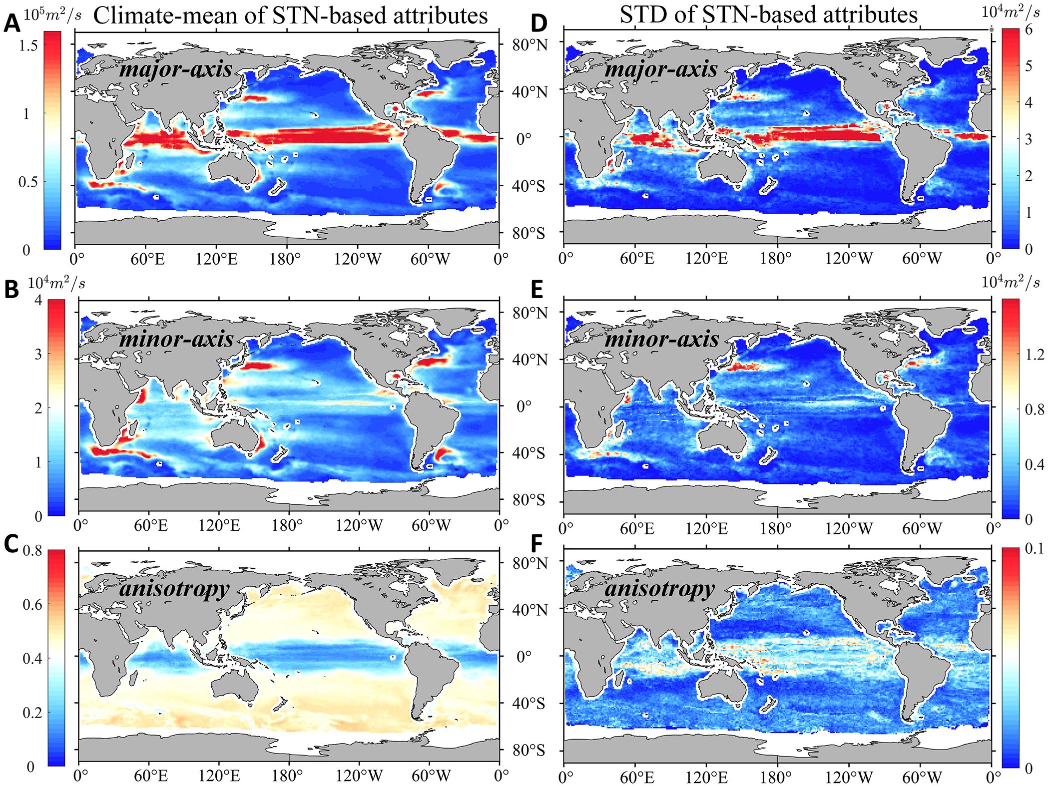
Figure 6. The climate-mean values of (A) major axis length, (B) minor axis length, (C) anisotropy, and the corresponding STD values (D-F) during 2006-2017 based on STN method. Results show the predictive skill of the STN model.

Three machine learning models show varying performance in predicting the temporal variations of three attributes. The RF model performs best for the axes, while the STN model outperforms both RF and CNN in minimizing the NRMSE between particle-based time series and predicted time series of mixing anisotropy at each grid point from 2006 to 2017. As shown in Figures 7A–D, the RF model accurately predicts the time series variations of global major and minor axis in the off-equatorial region (latitudes beyond ±15°). The zonally averaged correlation of major axis generally ranges from 0.55 to 0.8 across all the latitudes, while the correlation for minor axis exhibits more fluctuation, with values ranging from 0.5 to 0.7 in mid-high latitudes and lower values near the equator. Although all three models struggle to predict the temporal correlation of anisotropy, the STN model successfully captures its magnitude variation, with zonally averaged NRMSE remaining below 0.23 across mid-high latitudes (Figures 7E, F). In contrast, the RF and CNN models show higher zonally averaged NRMSE of 0.3 and 0.32, respectively. Given the small NSTD values of particle-based anisotropy in mid-high latitudes (Figure 5C), temporal variation in the equatorial region deserves further attention. We also quantify the global percentage of temporal correlation coefficients exceeding 0.5 and NRMSE below 0.4 for different models predicting the mixing-ellipse attributes (Table 1).

Figure 7

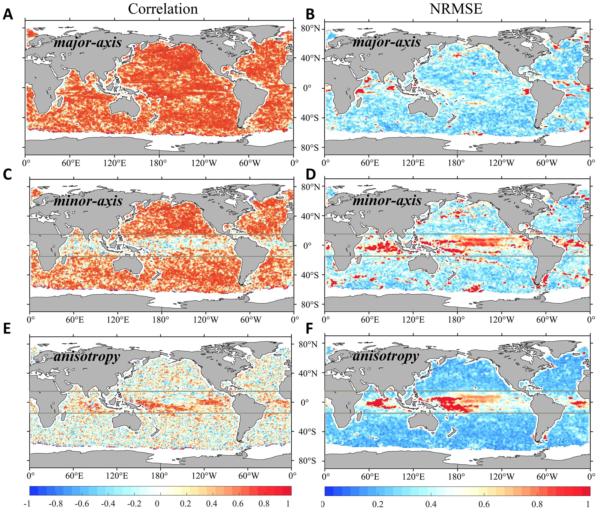
Figure 7. The correlation coefficients (left panel) and NRMSE (right panel) between particle-based and machine learning (ML)-based time series at global grid points spanning from 2006-2017 for (A, B) major axis, (C, D) minor axis and (E, F) mixing anisotropy. (A-D) shows the predictive skill of RF model and (E, F) shows the predictive skill of STN model. The zonal gray lines indicate those region within 15°N and 15°S. Dots in (A, C, E) indicate points where the correlation coefficient passes the 95% confidence level.

Table 1

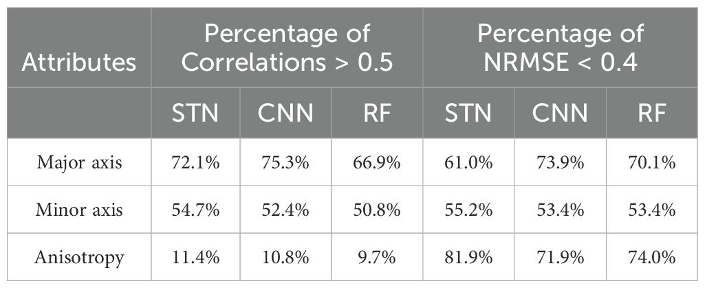
Table 1. Global percentage of correlation coefficients > 0.5 and NRMSE < 0.4 for time series predictions of three attributes using machine learning methods (refer to Figure 7).

The STN model shows clear advantages over the RF and CNN models in predicting the spatial structure of three attributes, particularly for mixing anisotropy (Figure 8). For the major axis, all models achieve high performance, with global spatial correlation coefficients above 0.85 and NRMSE around 0.4 for all years. Minor axis shows correlation ranging from 0.51 to 0.8, with NRMSE between 0.5 and 0.78. For mixing anisotropy, the correlation ranges from 0.47 to 0.7, with NRMSE between 0.26 and 0.35. The STN model increased the spatial correlation of annual anisotropy predictions by 0.08 compared to the RF and CNN models, while reducing NRMSE by 0.06. In certain years, STN and CNN models slightly outperform RF model, likely due to their use of predictor images that incorporate non-local flow information, which aids in predicting regions with larger mixing nonlocality (Guan et al., 2022). Furthermore, the STN model enhances anisotropy predictions by incorporating an adaptive spatial attention mechanism to learn spatial transformations, offering an advantage over traditional models.

Figure 8

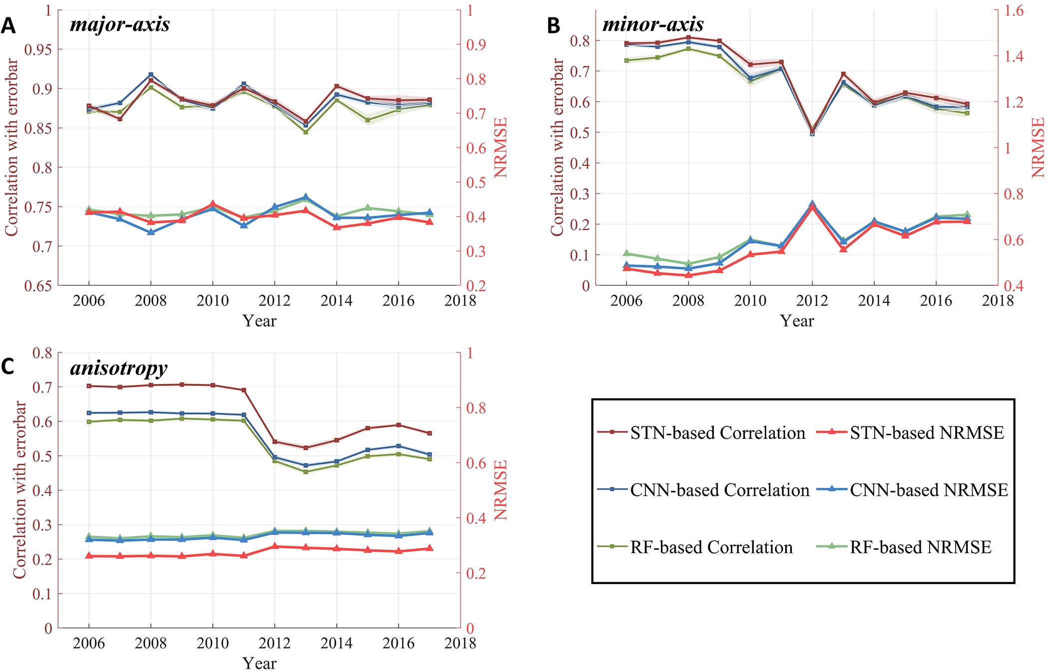
Figure 8. Spatial correlation and Normalized Root Mean Square Error (NRMSE) between particle-based attributes of mixing ellipses and those from RF, CNN and STN methods. Results during 2006-2017 showcase the predictive skill for (A) major axis length, (B) minor axis length and (C) anisotropy, respectively. Error bars of correlation coefficients, represented by the shaded region, are uncertainties at the 95% confidence level inferred from a bootstrapping method (Guan et al., 2022). These uncertainties are too small to be clearly visible in the figures.

4 Discussion

4.1 Feature importance analysis

Feature importance ranking is a tool to measure the contributions of individual features (predictors) to the performance of machine learning model (Lakshmanan et al., 2015; Yu et al., 2021). We employed permutation feature importance method to elucidate the relative importance of each predictor in predicting the predictand (Breiman, 2001; McGovern et al., 2019; Greenhill et al., 2024). Based on an already-trained model with all features, we randomly permute the values of a predictor multiple times, effectively breaking the statistical relation between the predictor and the predictand, and then evaluate how much the model performance deteriorates. A feature’s permutation importance is evaluated by calculating the difference of the NRMSE or correlation coefficients (R) between the experiment with features intact and that with features permuted. In other words, we rank the relative importance based on the following two metrics, ΔRMSE = NRMSE_permute − NRMSE_all and ΔR = R_all − R_permute, where ·_all denotes the variable from the experiments with features intact and ·_permute refers to the experiment with features permuted.

We evaluated the feature importance rankings for predicting the major axis, minor axis, and anisotropy of mixing ellipses using all three models. The values of ΔRMSE and ΔR for each model are shown in Figure 9. The rankings based on these metrics are consistent across the models. For the STN model (Figures 9A, B), u_rms and L_eddy have the greatest impact on predicting the major axis and mixing anisotropy. This aligns with eddy mixing length theory (Taylor, 1915), where eddy diffusivity is proportional to the product of u_rms and mixing length. Previous studies have assumed that mixing length scales with L_eddy (Stammer, 1998; Eden and Greatbatch, 2008; Bates et al., 2014) and Klocker and Abernathey (2014) confirmed that this theory is reasonable for weak mean flows. For the minor axis, u_rms and additional factor γ, proportional to u_rms/L_eddy (Equation 11) in SMLT, ranks the first and second. Among the four predictors, $\left|C_w-\right|\mathbf{\text{U}}\Vert$ consistently ranks as the least important for predicting the axes but ranks third for anisotropy. Interestingly, in the CNN model, γ ranks as the second-most important predictor for anisotropy, and in the RF model, it ranks third. This difference likely arises from the distinct architectures and data processing algorithms of these models.

Figure 9

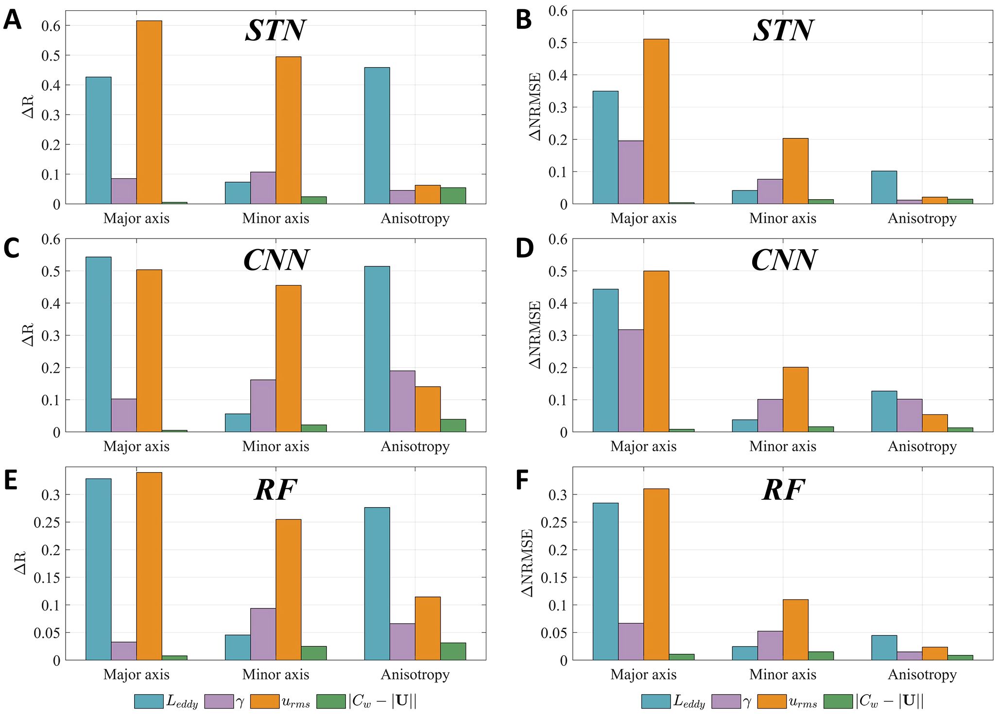
Figure 9. Permutation tests of global feature importance for (A, B) STN, (C, D) CNN and (E, F) RF models. Feature importance is analyzed using two metrics: (A, C, E) correlation coefficients difference (ΔR) and (B, D, F) NRMSE difference (ΔRMSE) between the experiment with features intact and that with features permuted.

Compared to the global result (Figure 9), the feature importance rankings for predicting minor axis within the jet region show slight variations (not shown). The jet region is defined as the area where $\left|C_w-\right|\mathbf{\text{U}}\Vert$ values rank in the top 10% globally. For instance, based on ΔR values, the importance ranking of $\left|C_w-\right|\mathbf{\text{U}}\Vert$ rises from fourth to third place in the RF model. The ratio of ΔRMSE values between |C_w −|U|| and L_eddy increases from 32.2%, 61.9% and 42.8% in the global analysis to 53%, 72.5% and 99.7% in the jet region for STN, CNN and RF, respectively. This finding is not surprising given that SMLT is formulated to capture the cross-stream mixing suppression phenomenon due to eddies propagating relative to the mean flow ($\left|C_w-\right|\mathbf{\text{U}}\Vert \ne \mathbf{0}$).

4.2 Equatorial analysis

Although RF, CNN and STN models well predict the spatiotemporal features of major axis throughout the ocean, they struggle to capture the minor axis and anisotropy in the equatorial region. We explored the following alternative settings of the models (12-Year model), with no improvement found. One, we use zonal and meridional eddy phase speed instead of along-stream eddy phase speed as predictors. Two, recognizing that eddies can be asymmetric (Liu et al., 2017; Tang et al., 2020), we use two new predictors (dominant zonal length scale and meridional length scale) to replace the single eddy size L_eddy in the predictor group. Three, we train the machine learning model only in the equatorial region.

Instead, we found that model performance in predicting temporal variation can be significantly enhanced by adjusting the temporal duration of the training set. The 2-Year model effectively captures the magnitude and temporal variability of mixing-ellipse attributes within the northern equatorial central Pacific (120°W-170°W, 0°-15°N), though the 12-Year model does not (Figure 10). Specifically, the spatially averaged correlation coefficients and NRMSE values between particle-based minor-axis or anisotropy time series and those predicted by 12-Year and 2-Year models are shown in Table 2. For instance, results from the STN model show an increase in correlation from 0.1 (0.01) to 0.58 (0.59) and a decrease in NRMSE from 0.71 (0.63) to 0.58 (0.48) when predicting minor axis (anisotropy).

Figure 10

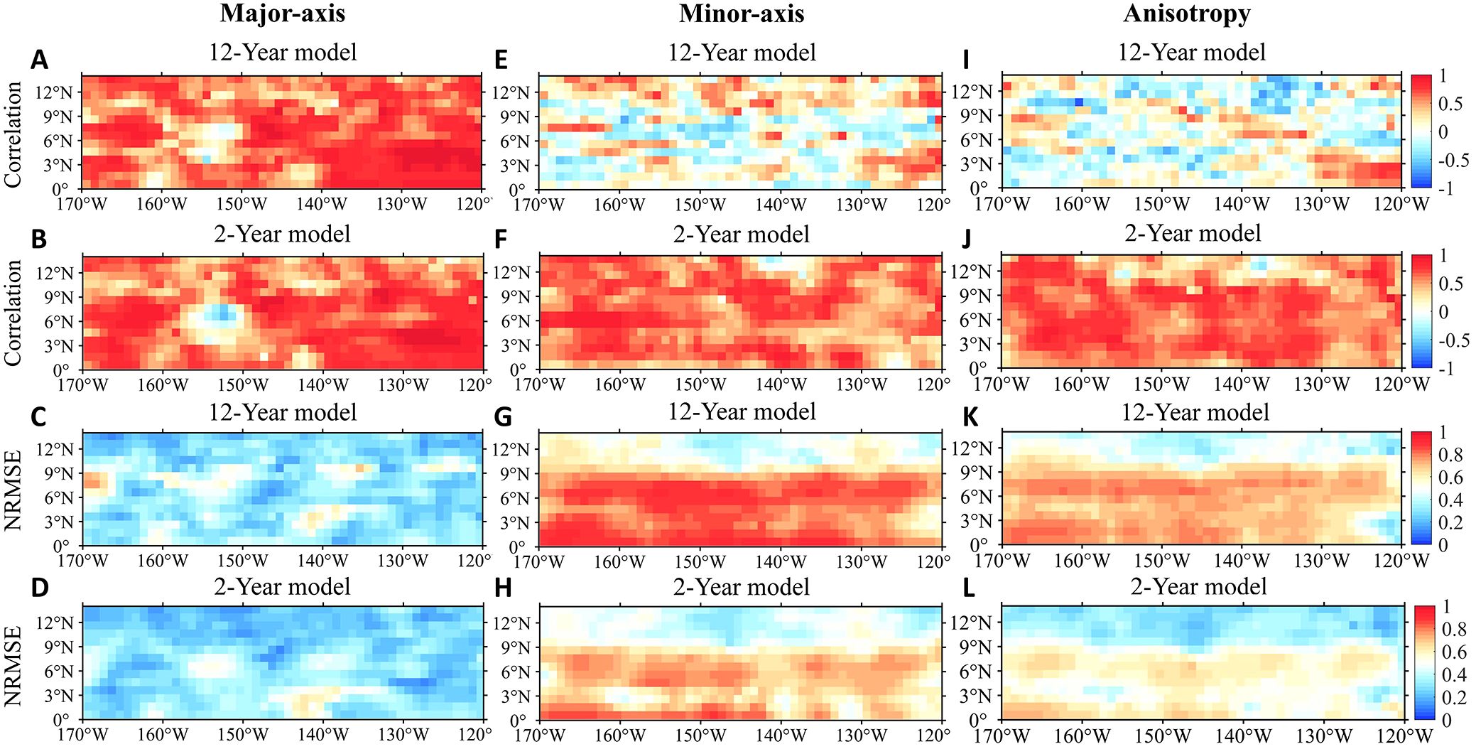
Figure 10. Time series correlation and NRMSE between particle-based attributes and that from STN-based 12-Year model or STN-based 2-Year model in the region ranging from 120°W-170°W, 0°-15°N. (A, B, E, F, I, J) Correlation and (C, D, G, H, K, L) NRMSE. (A-D) Major axis, (E-H) minor axis and (I-L) mixing anisotropy. Results from 12-Year model (A, C, E, G, I, K) and 2-Year model (B, D, F, H, J, L).

Table 2

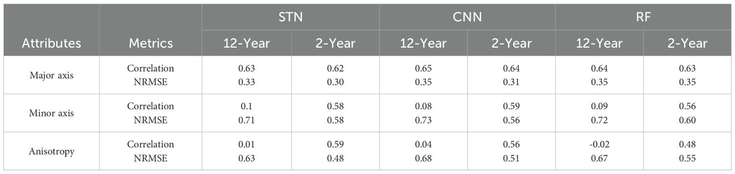
Table 2. Regionally averaged correlation coefficients and NRMSE for time series predictions of mixing-ellipse attributes using different machine learning models and training durations (refer to Figure 10).

Testing various training periods revealed that a 2- or 3-year period yielding the best results, likely because it aligns with the regional climate state. Previous studies have categorized ENSO events into types such as low-frequency and quasi-biennial, typically spanning 2-7 years per cycle (Hope et al., 2017; Santoso et al., 2017; Wang and Ren, 2020; Wang et al., 2023). ENSO’s warm phase (El Niño) and cold phase (La Niña) exhibit distinct dynamic processes and spatiotemporal characteristics. Therefore, a 2- or 3-year period likely represents a single ENSO phase or one climate state. If the training dataset contains data from the same specific climate state, prediction accuracy can be improved. Conversely, a dataset including data from multiple climate states may average out effects, potentially reducing the performance of machine learning models.

Several assumptions inherent in SMLT may also contribute to the predictive results in the equatorial regions. One, in contrast to the single-wavenumber limit, the realistic equatorial eddy field comprises motions with a wide range of wavenumbers and phase speeds, including westward Rossby waves, eastward Kelvin waves and tropical instability waves (which contains Rossby and Yanai modes; see, e.g., Liu et al. (2019)). Two, the constant mean flow assumption, inherent in SMLT, is inconsistent with the presence of strong alternating zonal currents here, such as the North Equatorial Current and the North Equatorial Counter Current.

There are potential avenues to further improve the machine learning prediction of mixing ellipses. One could incorporate eddies and mean flow properties from surrounding regions as predictors to take into account mixing nonlocality (Liu et al., 2023; Flierl and Souza, 2024). More machine learning algorithms can be explored in predicting mixing ellipses, such as the Adversarial Sparse Transformer (Wu et al., 2020; Xue and Salim, 2023). In addition, studying the underlying dynamical processes of equatorial eddy mixing may help identify additional predictors (e.g., climate indices) and design more physically informed machine learning models.

5 Summary

In this study, we first estimated the spatio-temporal variability of realistic eddy mixing ellipses at the global surface, focusing on their major axis, minor axis and anisotropy, using the Lagrangian single-particle method and satellite altimetry data. Our results reveal that mixing ellipses have significant spatio-temporal variability across the global ocean, and their morphology is closely linked to the mean flow and EKE in eddy-rich and energetic ocean regions.

Besides estimation, we evaluated the potential of machine learning algorithms, STN, CNN and RF, in representing and predicting particle-based mixing ellipses. Our results indicate that RF outperforms both CNN and STN in representing the spatio-temporal variability of mixing ellipses. Regarding the predictive skill, all three algorithms prove effective in predicting the spatio-temporal features of global axes. For instance, the global spatial correlation of annual-mean major (minor) axis predicted by STN ranges from 0.85 (0.5) to 0.92 (0.81) for all years considered, and the global spatially averaged temporal correlation coefficient is 0.62 (0.48) at the 95% confidence level. Furthermore, the STN model significantly improved the accuracy of predicting the spatial structure and magnitudes of mixing anisotropy, with spatial correlation values between 0.52 and 0.7 and NRMSE below 0.26.

We also assessed the feature importance rankings of four variables in predicting three mixing-ellipse attributes. Across three models, the eddy velocity magnitude (u_rms) and eddy size (L_eddy) were consistently identified as the most important predictors for the major axis and mixing anisotropy, while for u_rms and eddy decorrelation time scale γ were the top two predictors for predicting minor axis, aligning with eddy mixing length theory. Additionally, by adjusting the selection of training set, we found that training the models with a temporal duration of 2 or 3 years, aligned with ENSO timescale, improved predictions in the northern equatorial central Pacific region compared to models trained with a 12-year duration. This resulted in the spatially averaged correlation values for predicting the minor axis and anisotropy increased by over 0.5, while the NRMSE decreased by more than 0.15.

The significant variability of eddy mixing ellipses identified here indicates the need of appropriately choosing subgrid eddy diffusivity tensor and anisotropy in coarse-resolution models. Our findings show the potential of using machine learning models to predict eddy mixing ellipses. Based on instability theories, eddy properties are linked with the large-scale ocean state (Smith, 2007; Tulloch et al., 2011). Consistently, Xie et al. (2023) found that using the large-scale fields readily available in coarse-resolution models as predictors, machine learning models can well predict cross-slope isopycnal eddy diffusivity. Next, one could explore using the large-scale fields instead of eddy properties to predict eddy mixing ellipses. This effort would lead to practically useful parameterization schemes of eddy ellipses and implement in coarse-resolution models.

Data availability statement

The datasets presented in this study can be found in online repositories. The names of the repository/repositories and accession number(s) can be found below: https://zenodo.org/records/14258059.

Author contributions

TJ: Data curation, Formal analysis, Investigation, Methodology, Visualization, Writing – original draft. RC: Conceptualization, Data curation, Investigation, Methodology, Supervision, Writing – original draft, Funding acquisition, Project administration, Resources, Writing – review & editing. CL: Investigation, Writing – review & editing. CQ: Investigation, Writing – review & editing. CZ: Writing – review & editing, Funding acquisition. MH: Methodology, Writing – review & editing, Funding acquisition.

Funding

The author(s) declare financial support was received for the research, authorship, and/or publication of this article. The work was supported by the National Natural Science Foundation of China through 42076007 and 42476007.

Acknowledgments

We thank Guangchuang Zhang for his technical assistance about eddy diffusivity estimates.

Conflict of interest

The authors declare that the research was conducted in the absence of any commercial or financial relationships that could be construed as a potential conflict of interest.

Generative AI statement

The author(s) declare that no Generative AI was used in the creation of this manuscript.

Publisher’s note

All claims expressed in this article are solely those of the authors and do not necessarily represent those of their affiliated organizations, or those of the publisher, the editors and the reviewers. Any product that may be evaluated in this article, or claim that may be made by its manufacturer, is not guaranteed or endorsed by the publisher.

Supplementary material

The Supplementary Material for this article can be found online at: https://www.frontiersin.org/articles/10.3389/fmars.2024.1506419/full#supplementary-material

References

Abernathey R., Ferreira D., Klocker A. (2013). Diagnostics of isopycnal mixing in a circumpolar channel. Ocean Model. 72, 1–16. doi: 10.1016/j.ocemod.2013.07.004

Crossref Full Text | Google Scholar

Abernathey R., Haller G. (2018). Transport by Lagrangian vortices in the eastern Pacific. J. Phys. Oceanogr. 48, 667–685. doi: 10.1175/JPO-D-17-0102.1

Crossref Full Text | Google Scholar

Abernathey R. P., Marshall J. (2013). Global surface eddy diffusivities derived from satellite altimetry. J. Geophys. Res.: Oceans 118, 901–916. doi: 10.1002/jgrc.20066

Crossref Full Text | Google Scholar

Bachman S. D., Fox-Kemper B., Bryan F. O. (2020). A diagnosis of anisotropic eddy diffusion from a high-resolution global ocean model. J. Adv. Model. Earth Syst. 12, e2019MS001904. doi: 10.1029/2019MS001904

Crossref Full Text | Google Scholar

Bates M., Tulloch R., Marshall J., Ferrari R. (2014). Rationalizing the spatial distribution of mesoscale eddy diffusivity in terms of mixing length theory. J. Phys. Oceanogr. 44, 1523–1540. doi: 10.1175/JPO-D-13-0130.1

Crossref Full Text | Google Scholar

Berloff P. S., McWilliams J. C., Bracco A. (2002). Material transport in oceanic gyres. part i: Phenomenology. J. Phys. Oceanogr. 32, 764–796. doi: 10.1175/1520-0485(2002)032<0764:MTIOGP>2.0.CO;2

Crossref Full Text | Google Scholar

Bovenschen T. (2021). The influence of tides on anisotropic eddy diffusivities in the Labrador sea using a Lagrangian framework. Utrecht University, Netherlands. Available online at: https://studenttheses.uu.nl/handle/20.500.12932/40938.

Google Scholar

Breiman L. (2001). Random forests. Mach. Learn. 45, 5–32. doi: 10.1023/A:1010933404324

Crossref Full Text | Google Scholar

Busecke J. J., Abernathey R. P. (2019). Ocean mesoscale mixing linked to climate variability. Sci. Adv. 5, eaav5014. doi: 10.1126/sciadv.aav5014

PubMed Abstract | Crossref Full Text | Google Scholar

Cao C., Bao L., Gao G., Liu G., Zhang X. (2024). A novel method for ocean wave spectra retrieval using deep learning from sentinel-1 wave mode data. IEEE Trans. Geosci. Remote Sens 62, 1–16. doi: 10.1109/TGRS.2024.3369080

Crossref Full Text | Google Scholar

Chen R., Gille S. T., McClean J. L. (2017). Isopycnal eddy mixing across the Kuroshio Extension: Stable versus unstable states in an eddying model. J. Geophys. Res.: Oceans 122, 4329–4345. doi: 10.1002/2016JC012164

Crossref Full Text | Google Scholar

Chen R., McClean J. L., Gille S. T., Griesel A. (2014). Isopycnal eddy diffusivities and critical layers in the Kuroshio Extension from an eddying ocean model. J. Phys. Oceanogr. 44, 2191–2211. doi: 10.1175/JPO-D-13-0258.1

Crossref Full Text | Google Scholar

Chen R., Waterman S. (2017). Mixing nonlocality and mixing anisotropy in an idealized western boundary current jet. J. Phys. Oceanogr. 47, 3015–3036. doi: 10.1175/JPO-D-17-0011.1

Crossref Full Text | Google Scholar

Danabasoglu G., Marshall J. (2007). Effects of vertical variations of thickness diffusivity in an ocean general circulation model. Ocean Model. 18, 122–141. doi: 10.1016/j.ocemod.2007.03.006

Crossref Full Text | Google Scholar

Davis R. E. (1987). Modeling eddy transport of passive tracers. J. Mar. Res. 45, 635–666. doi: 10.1357/002224087788326803

Crossref Full Text | Google Scholar

Eden C., Greatbatch R. J. (2008). Towards a mesoscale eddy closure. Ocean Model. 20, 223–239. doi: 10.1016/j.ocemod.2007.09.002

Crossref Full Text | Google Scholar

Ferrari R., Nikurashin M. (2010). Suppression of eddy diffusivity across jets in the Southern Ocean. J. Phys. Oceanogr. 40, 1501–1519. doi: 10.1175/2010JPO4278.1

Crossref Full Text | Google Scholar

Flierl G. R., Souza A. N. (2024). On the non-local nature of turbulent fluxes of passive scalars. J. Fluid Mech. 986, A8. doi: 10.1017/jfm.2024.302

Crossref Full Text | Google Scholar

Foppert A., Donohue K. A., Watts D. R., Tracey K. L. (2017). Eddy heat flux across the a ntarctic c ircumpolar c urrent estimated from sea surface height standard deviation. J. Geophys. Res.: Oceans 122, 6947–6964. doi: 10.1002/2017JC012837

Crossref Full Text | Google Scholar

Gao G., Bai Q., Zhang C., Zhang L., Yao L. (2023a). Dualistic cascade convolutional neural network dedicated to fully polsar image ship detection. ISPRS J. Photogramm. Remote Sens. 202, 663–681. doi: 10.1016/j.isprsjprs.2023.07.006

Crossref Full Text | Google Scholar

Gao G., Chen Y., Feng Z., Zhang C., Duan D., Li H., et al. (2024a). R-lrbpnet: A lightweight sar image oriented ship detection and classification method. Remote Sens. 16, 1533. doi: 10.3390/rs16091533

Crossref Full Text | Google Scholar

Gao G., Dai Y., Zhang X., Duan D., Guo F. (2023b). Adcg: A cross-modality domain transfer learning method for synthetic aperture radar in ship automatic target recognition. IEEE Trans. Geosci. Remote Sens. 61, 1–14. doi: 10.1109/TGRS.2023.3313204

Crossref Full Text | Google Scholar

Gao G., Yao B., Li Z., Duan D., Zhang X. (2024b). Forecasting of sea surface temperature in eastern tropical pacific by a hybrid multi-scale spatial-temporal model combining error correction map. IEEE Trans. Geosci. Remote Sens. 62, 1–22. doi: 10.1109/TGRS.2024.3353288

Crossref Full Text | Google Scholar

Gao G., Yao L., Li W., Zhang L., Zhang M. (2023c). Onboard information fusion for multisatellite collaborative observation: Summary, challenges, and perspectives. IEEE Geosci. Remote Sens. Mag. 11, 40–59. doi: 10.1109/MGRS.2023.3274301

Crossref Full Text | Google Scholar

Gao G., Zhang C., Zhang L., Duan D. (2023d). Scattering characteristic-aware fully polarized sar ship detection network based on a four-component decomposition model. IEEE Trans. Geosci. Remote Sens. 61, 1–22. doi: 10.1109/TGRS.2023.3336300

Crossref Full Text | Google Scholar

Gao G., Zhou P., Yao L., Liu J., Zhang C., Duan D. (2023e). A bi-prototype bdc metric network with lightweight adaptive task attention for few-shot fine-grained ship classification in remote sensing images. IEEE Trans. Geosci. Remote Sens. 61, 1–16. doi: 10.1109/TGRS.2023.3321533

Crossref Full Text | Google Scholar

Greenhill S., Druckenmiller H., Wang S., Keiser D. A., Girotto M., Moore J. K., et al. (2024). Machine learning predicts which rivers, streams, and wetlands the Clean Water Act regulates. Science 383, 406–412. doi: 10.1126/science.adi3794

PubMed Abstract | Crossref Full Text | Google Scholar

Griesel A., McClean J., Gille S., Sprintall J., Eden C. (2014). Eulerian and Lagrangian isopycnal eddy diffusivities in the southern ocean of an eddying model. J. Phys. Oceanogr. 44, 644–661. doi: 10.1175/JPO-D-13-039.1

Crossref Full Text | Google Scholar

Guan W., Chen R., Zhang H., Yang Y., Wei H. (2022). Seasonal surface eddy mixing in the Kuroshio Extension: Estimation and machine learning prediction. J. Geophys. Res.: Oceans 127, e2021JC017967. doi: 10.1029/2021JC017967

Crossref Full Text | Google Scholar

Guan Y., Zhang X., Chen S., Liu G., Jia Y., Zhang Y., et al. (2023). Fishing vessel classification in sar images using a novel deep learning model. IEEE Trans. Geosci. Remote Sens. 61, 1–21. doi: 10.1109/TGRS.2023.3312766

Crossref Full Text | Google Scholar

Haigh M., Sun L., McWilliams J. C., Berloff P. (2021). On eddy transport in the ocean. Part I: The diffusion tensor. Ocean Model. 164, 101831. doi: 10.1016/j.ocemod.2021.101831

Crossref Full Text | Google Scholar

Ho T. K. (1995). “Random decision forests,” in Proceedings of 3rd international conference on document analysis and recognition (IEEE), Vol. 1. 278–282. doi: 10.1109/ICDAR.1995.598994

Crossref Full Text | Google Scholar

Holmes R., Groeskamp S., Stewart K., McDougall T. (2022). Sensitivity of a coarse-resolution global ocean model to a spatially variable neutral diffusivity. J. Adv. Model. Earth Syst. 14, e2021MS002914. doi: 10.1029/2021MS002914

Crossref Full Text | Google Scholar

Hope P., Henley B. J., Gergis J., Brown J., Ye H. (2017). Time-varying spectral characteristics of ENSO over the Last Millennium. Climate Dynam. 49, 1705–1727. doi: 10.1007/s00382-016-3393-z

Crossref Full Text | Google Scholar

Jaderberg M., Simonyan K., Zisserman A., Kavukcuoglu K. (2015). Spatial transformer networks. Adv. Neural Inf. Process. Syst. 2, 2017-2025. doi: 10.5555/2969442.2969465

Crossref Full Text | Google Scholar

Kamenkovich I., Berloff P., Haigh M., Sun L., Lu Y. (2021). Complexity of mesoscale eddy diffusivity in the ocean. Geophys. Res. Lett. 48, e2020GL091719. doi: 10.1029/2020GL091719

Crossref Full Text | Google Scholar

Kamenkovich I., Berloff P., Pedlosky J. (2009). Anisotropic material transport by eddies and eddydriven currents in a model of the North Atlantic. J. Phys. Oceanogr. 39, 3162–3175. doi: 10.1175/2009JPO4239.1

Crossref Full Text | Google Scholar

Kamenkovich I., Rypina I. I., Berloff P. (2015). Properties and origins of the anisotropic eddyinduced transport in the North Atlantic. J. Phys. Oceanogr. 45, 778–791. doi: 10.1175/JPO-D-14-0164.1

Crossref Full Text | Google Scholar

Klocker A., Abernathey R. (2014). Global patterns of mesoscale eddy properties and diffusivities. J. Phys. Oceanogr. 44, 1030–1046. doi: 10.1175/JPO-D-13-0159.1

Crossref Full Text | Google Scholar

Kong H., Jansen M. F. (2021). The impact of topography and eddy parameterization on the simulated Southern Ocean circulation response to changes in surface wind stress. J. Phys. Oceanogr. 51, 825–843. doi: 10.1175/JPO-D-20-0142.1

Crossref Full Text | Google Scholar

Koszalka I. M., LaCasce J. H. (2010). Lagrangian analysis by clustering. Ocean Dynam. 60, 957–972. doi: 10.1007/s10236-010-0306-2

Crossref Full Text | Google Scholar

Lagerloef G. S., Mitchum G. T., Lukas R. B., Niiler P. P. (1999). Tropical pacific near-surface currents estimated from altimeter, wind, and drifter data. J. Geophys. Res.: Oceans 104, 23313–23326. doi: 10.1029/1999JC900197

Crossref Full Text | Google Scholar

Lakshmanan V., Karstens C., Krause J., Elmore K., Ryzhkov A., Berkseth S. (2015). Which polarimetric variables are important for weather/no-weather discrimination? J. Atmos. Ocean. Technol. 32, 1209–1223. doi: 10.1175/JTECH-D-13-00205.1

Crossref Full Text | Google Scholar

Liu C., Köhl A., Stammer D. (2012). Adjoint-based estimation of eddy-induced tracer mixing parameters in the global ocean. J. Phys. Oceanogr. 42, 1186–1206. doi: 10.1175/JPO-D-11-0162.1

Crossref Full Text | Google Scholar

Liu C., Wang X., Köhl A., Wang F., Liu Z. (2019). The northeast-southwest oscillating equatorial mode of the tropical instability wave and its impact on equatorial mixing. Geophys. Res. Lett. 46, 218–225. doi: 10.1029/2018GL080226

Crossref Full Text | Google Scholar

Liu M., Chen R., Guan W., Zhang H., Jing T. (2023). Nonlocality of scale-dependent eddy mixing at the Kuroshio Extension. Front. Mar. Sci. 10. doi: 10.3389/fmars.2023.1137216

Crossref Full Text | Google Scholar

Liu Y., Dong C., Liu X., Dong J. (2017). Antisymmetry of oceanic eddies across the kuroshio over a shelfbreak. Sci. Rep. 7, 6761. doi: 10.1038/s41598-017-07059-1

PubMed Abstract | Crossref Full Text | Google Scholar

McGovern A., Lagerquist R., Gagne D. J., Jergensen G. E., Elmore K. L., Homeyer C. R., et al. (2019). Making the black box more transparent: Understanding the physical implications of machine learning. Bull. Am. Meteorol. Soc. 100, 2175–2199. doi: 10.1175/BAMS-D-18-0195.1

Crossref Full Text | Google Scholar

Mirmohammadsadeghi M., Hanna S. S., Cabric D. (2017). “Modulation classification using convolutional neural networks and spatial transformer networks,” in 2017 51st Asilomar Conference on Signals, Systems, and Computers (IEEE), 936–939. doi: 10.1109/ACSSC.2017.8335486

Crossref Full Text | Google Scholar

Nummelin A., Busecke J. J., Haine T. W., Abernathey R. P. (2021). Diagnosing the scale-and spacedependent horizontal eddy diffusivity at the global surface ocean. J. Phys. Oceanogr. 51, 279–297. doi: 10.1175/JPO-D-19-0256.1

Crossref Full Text | Google Scholar

Qiu B., Chen S., Schneider N., Taguchi B. (2014). A coupled decadal prediction of the dynamic state of the Kuroshio Extension system. J. Climate 27, 1751–1764. doi: 10.1175/JCLI-D-13-00318.1

Crossref Full Text | Google Scholar

Raney R. K. (2016). Comparing compact and quadrature polarimetric sar performance. IEEE Geosci. Remote Sens. Lett. 13, 861–864. doi: 10.1109/LGRS.2016.2550863

Crossref Full Text | Google Scholar

Rosso I., Hogg A. M., Kiss A. E., Gayen B. (2015). Topographic influence on submesoscale dynamics in the Southern Ocean. Geophys. Res. Lett. 42, 1139–1147. doi: 10.1002/2014GL062720

Crossref Full Text | Google Scholar

Rypina I. I., Kamenkovich I., Berloff P., Pratt L. J. (2012). Eddy-induced particle dispersion in the near-surface North Atlantic. J. Phys. Oceanogr. 42, 2206–2228. doi: 10.1175/JPO-D-11-0191.1

Crossref Full Text | Google Scholar

Sallée J., Speer K., Rintoul S. (2011). Mean-flow and topographic control on surface eddy-mixing in the Southern Ocean. J. Mar. Res. 69, 753–777. doi: 10.1357/002224011799849408

Crossref Full Text | Google Scholar

Santoso A., Mcphaden M. J., Cai W. (2017). The defining characteristics of ENSO extremes and the strong 2015/2016 El Niño. Rev. Geophys. 55, 1079–1129. doi: 10.1002/2017RG000560

Crossref Full Text | Google Scholar

Shao W., Duan B., Hu Y., Zuo J., Jiang X. (2023). Analysis of mesoscale eddy in the Nordic seas and Barents sea using multi-satellite data. J. Sea Res. 196, 102443. doi: 10.1016/j.seares.2023.102443

Crossref Full Text | Google Scholar

Simmons H. L., Jayne S. R., Laurent L. C. S., Weaver A. J. (2004). Tidally driven mixing in a numerical model of the ocean general circulation. Ocean Model. 6, 245–263. doi: 10.1016/S1463-5003(03)00011-8

Crossref Full Text | Google Scholar

Sinclair M., Schuh A., Hahn K., Petersen K., Bai Y., Batten J., et al. (2022). Atlas-istn: joint segmentation, registration and atlas construction with image-and-spatial transformer networks. Med. Image Anal. 78, 102383. doi: 10.1016/j.media.2022.102383

PubMed Abstract | Crossref Full Text | Google Scholar

Smith K. S. (2007). The geography of linear baroclinic instability in Earth’s oceans. J. Mar. Res. 65, 655–683. doi: 10.1357/002224007783649484

Crossref Full Text | Google Scholar

Stammer D. (1998). On eddy characteristics, eddy transports, and mean flow properties. J. Phys. Oceanogr. 28, 727–739. doi: 10.1175/1520-0485(1998)028<0727:OECETA>2.0.CO;2

Crossref Full Text | Google Scholar

Su H., Li W., Yan X.-H. (2018). Retrieving temperature anomaly in the global subsurface and deeper ocean from satellite observations. J. Geophys. Res.: Oceans 123, 399–410. doi: 10.1002/2017JC013631

Crossref Full Text | Google Scholar

Tang Q., Gulick S. P., Sun J., Sun L., Jing Z. (2020). Submesoscale features and turbulent mixing of an oblique anticyclonic eddy in the gulf of alaska investigated by marine seismic survey data. J. Geophys. Res.: Oceans 125, e2019JC015393. doi: 10.1029/2019JC015393

Crossref Full Text | Google Scholar

Taylor G. I. (1915). “Eddy motion in the atmosphere,” in Philosophical Transactions of the Royal Society of London, vol. 215, 1–26. doi: 10.1098/rsta.1915.0001

Crossref Full Text | Google Scholar

Thompson A. F., Garabato A. C. N. (2014). Equilibration of the antarctic circumpolar current by standing meanders. J. Phys. Oceanogr. 44, 1811–1828. doi: 10.1175/JPO-D-13-0163.1

Crossref Full Text | Google Scholar

Tulloch R., Marshall J., Hill C., Smith K. S. (2011). Scales, growth rates, and spectral fluxes of baroclinic instability in the ocean. J. Phys. Oceanogr. 41, 1057–1076. doi: 10.1175/2011JPO4404.1

Crossref Full Text | Google Scholar

Vallis G. K. (2006). Atmospheric and oceanic fluid dynamics: Fundamentals and large-Scale circulation (Cambridge University Press). doi: 10.1017/9781107588417

Crossref Full Text | Google Scholar

Wang R., Ren H.-L. (2020). Understanding key roles of two ENSO modes in spatiotemporal diversity of ENSO. J. Climate 33, 6453–6469. doi: 10.1175/JCLI-D-19-0770.1

Crossref Full Text | Google Scholar

Wang Y., Yang R., Ding R., Cao J. (2023). The impact of the extratropical north pacific on the quasibiennial variability in ENSO. Climate Dynam. 61, 4061–4078. doi: 10.1007/s00382-023-06792-w

Crossref Full Text | Google Scholar

Wei H., Wang Y. (2021). Full-depth scalings for isopycnal eddy mixing across continental slopes under upwelling-favorable winds. J. Adv. Model. Earth Syst. 13, e2021MS002498. doi: 10.1029/2021MS002498

Crossref Full Text | Google Scholar

Witter D. L., Chelton D. B. (1998). Eddy–mean flow interaction in zonal oceanic jet flow along zonal ridge topography. J. Phys. Oceanogr. 28, 2019–2039. doi: 10.1175/1520-0485(1998)028<2019:EMFIIZ>2.0.CO;2

Crossref Full Text | Google Scholar

Wolfram P. J., Ringler T. D., Maltrud M. E., Jacobsen D. W., Petersen M. R. (2015). Diagnosing isopycnal diffusivity in an eddying, idealized midlatitude ocean basin via Lagrangian, in situ, global, high-performance particle tracking (LIGHT). J. Phys. Oceanogr. 45, 2114–2133. doi: 10.1175/JPO-D-14-0260.1

Crossref Full Text | Google Scholar

Wu S., Xiao X., Ding Q., Zhao P., Wei Y., Huang J. (2020). Adversarial sparse transformer for time series forecasting. Adv. Neural Inf. Process. Syst. 33, 17105–17115. doi: 10.5555/3495724.3497159

Crossref Full Text | Google Scholar

Xie C., Wei H., Wang Y. (2023). Impact of parameterized isopycnal diffusivity on shelf-ocean exchanges under upwelling-favorable winds: Offline tracer simulations augmented by Artificial Neural Network. J. Adv. Model. Earth Syst. 15, e2022MS003424. doi: 10.1029/2022MS003424

Crossref Full Text | Google Scholar

Xue H., Salim F. D. (2023). Promptcast: A new prompt-based learning paradigm for time series forecasting. IEEE Trans. Knowledge Data Eng. doi: 10.1109/TKDE.2023.3342137

Crossref Full Text | Google Scholar

Yu F., Wei C., Deng P., Peng T., Hu X. (2021). Deep exploration of random forest model boosts the interpretability of machine learning studies of complicated immune responses and lung burden of nanoparticles. Sci. Adv. 7, eabf4130. doi: 10.1126/sciadv.abf4130

PubMed Abstract | Crossref Full Text | Google Scholar

Zhang G., Chen R., Li X., Li L., Wei H., Guan W. (2023c). Temporal variability of global surface eddy diffusivities: Estimates and machine learning prediction. J. Phys. Oceanogr. 53, 1711–1730. doi: 10.1175/JPO-D-22-0251.s1

Crossref Full Text | Google Scholar

Zhang G., Chen R., Li L., Wei H., Sun S. (2023b). Global trends in surface eddy mixing from satellite altimetry. Front. Mar. Sci. 10. doi: 10.3389/fmars.2023.1157049

Crossref Full Text | Google Scholar

Zhang X., Gao G., Chen S.-W. (2024b). Polarimetric autocorrelation matrix: A new tool for joint characterizing of target polarization and doppler scattering mechanism. IEEE Trans. Geosci. Remote Sens. 62, 1–22. doi: 10.1109/TGRS.2024.3398632

Crossref Full Text | Google Scholar

Zhang L., Gao G., Chen C., Gao S., Yao L. (2022). Compact polarimetric synthetic aperture radar for target detection: A review. IEEE Geosci. Remote Sens. Mag. 10, 115–152. doi: 10.1109/MGRS.2022.3186904

Crossref Full Text | Google Scholar

Zhang C., Gao G., Liu J., Duan D. (2023a). Oriented ship detection based on soft thresholding and context information in sar images of complex scenes. IEEE Trans. Geosci. Remote Sens. 62, 1–15. doi: 10.1109/TGRS.2023.3340891

Crossref Full Text | Google Scholar

Zhang W., Wolfe C. L. (2022). On the vertical structure of oceanic mesoscale tracer diffusivities. J. Adv. Model. Earth Syst. 14, e2021MS002891. doi: 10.1029/2021MS002891

Crossref Full Text | Google Scholar

Zhang C., Zhang X., Gao G., Lang H., Liu G., Cao C., et al. (2024a). Development and application of ship detection and classification datasets: A review. IEEE Geosci. Remote Sens. Mag. 12, 12–45. doi: 10.1109/MGRS.2024.3450681

Crossref Full Text | Google Scholar