Experimental and theoretical studies of sea ice effects on internal solitary waves

Internal solitary waves in polar regions have attracted much interest recently. It is important to understand how sea ice affects them as this may have a profound influence on human activities and the environment. In this study, experiments on internal solitary waves with and without two types of sea ice (ice sheet and ice keel) are presented, as well as corresponding simulations using the Korteweg-de Vries (KdV) equation, the Benjamin-Ono (BO) equation, and the variable-coefficient Korteweg-de Vries (vKdV) equation, which is a derivation of the KdV equation. Comparison between experiments without sea ice and simulations using the KdV and BO equations proves the suitability of the former over the latter for this study. The experiments with sea ice and theoretical simulations using the vKdV equation provide evidence for wave deformation, oscillation occurring in the rear of the wave, and a decrease in amplitude. The latter suggests possibilities of energy dissipation or the emission of small amplitude linear waves. The sharp vertices of the ice result in occasional inconsistency with the vKdV predictions. Nonetheless, the vKdV equation is still suitable for modeling internal solitary waves under sea ice, giving generally accurate results that can assist further studies. This is the first time the vKdV equation has been applied to investigate the impacts of sea ice on internal solitary waves.

1 Introduction

Internal waves in the ocean, in contrast to surface waves, are within the water column in the stratified ocean and are often effectively modeled as layers of water of different densities. Unlike surface waves, internal waves are usually larger in wavelength and amplitude. The typical time and horizontal length scales of internal waves are hours and kilometers, and the vertical length scales can have the order of 10 meters (Munk, 1981). Linear internal waves are waves with very small amplitudes and can be described by linear theory. Nonlinear internal waves, on the other hand, usually have large enough amplitudes that nonlinear effects become important. As their name has indicated, they can only be described by nonlinear theory, and their propagation speeds are always larger than linear theory predicts. One type of nonlinear internal wave is called an internal solitary wave, which is well separated from the others because the non-hydrostatic dispersion balances nonlinearity during its propagation. Non-hydrostatic dispersion is an effect that tends to spread out the internal wave whereas the nonlinearity tends to steepen the wave. Since the two effects can be balanced, the waveform can be preserved and the wave can travel over a long distance.

Internal waves are one of the major causes of the variations in speed and density in the ocean over time. They also enable momentum and energy to pass from almost planar circulation in great measure to modest spatial fluctuations. The theoretical study of waves between layers of fluid began approximately 180 years ago (Stokes, 1847), whereas the earliest observation of internal waves, known as the “dead-water phenomenon”, carried out by Nansen (1902), took place at the end of the 19th century with the reason behind it explained in the next century by Ekman (1904). Yet the study was slowed down by the eruption of World War II and limited by technical challenges until the breakthrough of research instruments in the 1940s allowed it to be fostered. Along with this advance, the theories and methods of analysis experienced rapid development. Upon this basis, Garrett and Munk (GM) proposed a spectral model to explain the consistency of internal waves in both the scales of time and space (Garrett and Munk, 1972).

After this milestone, the direction of research has turned to sources, sinks, evolution, and interactions. It is believed that searching for areas where the internal wave field differs from the canonical GM spectrum can be a way to determine the sources and sinks of internal waves (Wunsch, 1976). In particular, the Arctic Ocean has demonstrated features that lead to the suggestion that it possesses such deviation (Morison et al., 1985). By analyzing the data from Yearsley (1966), Neshyba et al. (1972), Bernstein and Hunkins (1971), and Bernstein (1972), Morison (1986) discovered that although the slope of the internal wave spectra is conserved, there is a significant difference in the energy levels, being 5% to 33% smaller than the values given by the GM model. Levine et al. (1985) supported this with more data and evidence showing the likelihood of these energy levels was lower than those in ice-free oceans. It is thus important to examine internal waves under conditions simulating the Arctic Ocean when studying the sources and sinks of internal waves.

Apart from this, the influences of polar internal waves are also a sufficient reason for study. In the polar seas, internal waves have a non-negligible impact on the mixing between layers (D’Asaro and Morison, 1992; Fer, 2014; Kirillov, 2006) and, therefore, on the replacement of nutrients, as well as the progression of sea ice (Carr et al., 2019). Furthermore, they have an active participation in thermodynamics and circulation (Levine et al., 1985; Sandven and Johannessen, 1987). They have been found to be responsible for the curvature of sea ice (Czipott et al., 1991; Marchenko et al., 2010) and contribute to forming ice bands in the marginal ice zone (Muench et al., 1983; Saiki and Mitsudera, 2016). The effect of internal solitary waves on the Arctic ice edge is particularly worth noting, as the alterations of the ice edge are highlighted for purposes of maritime traffic, offshore operations, military marine activities, and their close relationship with climate change (Carr et al., 2019).

However, to date, most field research has assessed the integral influence of polar conditions involving ice and other oceanic parameters, whereas little study has been presented to illustrate the sole effects of each. Yet, the physical conditions and locations themselves cause difficulty in observation (Carr et al., 2019) while laboratory experiments benefit from a technological evolution that includes, but is not limited to, improved computational information processing and memorizing systems and equipment such as lasers (Sutherland et al., 2014). Hence, laboratory study has become a promising pathway for the investigation of internal waves in polar oceans and can be particularly valuable for theoretical studies, which would bring helpful analytical insights into and predictions of internal wave behavior. Ever since Ekman’s experiment on internal waves (Ekman, 1904), there have been numerous studies on internal waves in the laboratory. Experiments on sea ice and internal waves, in contrast, are much scarcer. The most recent research includes Carr et al. (2019) and Hartharn-Evans et al. (2024).

In terms of internal solitary wave modeling, there are a few well-established models. As a popular option, the Korteweg–de Vries (KdV) equation models the propagation of small amplitude (weakly nonlinear) waves in shallow water, accurate to at least the first order. Studies on KdV for internal solitary waves between layers of fluid began as early as 1876 (Wang, 2009), and for variable coefficients since 1981 (Grimshaw, 1981). The latter is called the variable-coefficient Korteweg–de Vries (vKdV) equation. The Benjamin–Ono (BO) equation presented by Benjamin (1966) and Ono (1975), on the other hand, is specially designed for deep water conditions.

In this paper, the experimental setup and the KdV, vKdV, and BO equations are detailed in the Materials and methods section. The results are presented in the Results section, including a comparison between the KdV and BO equations, as well as comparisons between theoretical and experimental observations. A discussion on the wide application of the KdV equation and an evaluation of the vKdV equation for studies on sea ice-impacted internal solitary waves are provided in the Discussion section.

2 Materials and methods

2.1 Experimental setup

The experiments can be divided into three groups: one group in the absence of sea ice for comparison between the KdV and BO models and two groups for the two types of sea ice whose effects on an internal solitary wave were examined.

The experiments were conducted in a water flume with an inner length of $1.90 m$ and an inner width of $0.15 m$ in a low-temperature laboratory the temperature of which is carefully monitored to be approximately $-5°\text{C}$ in order to prevent any formation or melting of ice within the flume. The water flume was set up as shown in Figure 1A, with a camera set to the side of the flume to record wave movements. A ruler is stuck to the side facing the camera to provide a reference of actual distances. There were two layers of water within the flume: 1) salty water with a density of ${\rho }_2=1.045g/c{m}^3$ filling up to $h_2=15 cm$ high and 2) fresh water with a density of ${\rho }_1=1.000g/c{m}^3$ above the salt water (see 2.2 Sea Ice for specific values of $h_1$). The freshwater was dyed beforehand to help distinguish between the salty and fresh water. To ensure minimal mixing, before adding the fresh water, a thin plastic foam sheet was attached to one end of the flume, floating on the surface of the salty water. The freshwater was then added to the sheet using a water pump. After that, a gate of equal width to the water flume was inserted near one end, and more fresh water was added to the same side. Two values for the total height of the fresh water on this side were applied in the experiments: 1) $h_{w1}=5\text{ cm}$ or 2) $h_{w2}=10\text{ cm}$, respectively, to produce two different wave amplitudes for comparison.

Figure 1

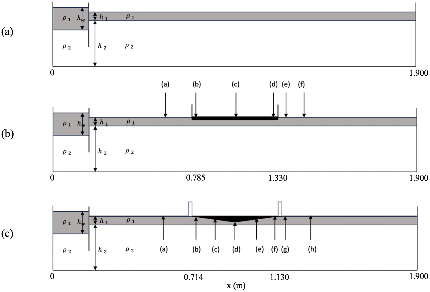
Figure 1. The setups for each experiment: (A) Experiments 1 and 2; (B) Experiments 3 and 4 with positions (a-f) labeled; (C) Experiment 5 with positions (a-h) labeled.

For experiments without sea ice (Experiments 1 and 2), an internal solitary wave was formed, while for experiments with ice, the ice must be placed as in Figures 1B, C before the wave was formed. An internal solitary wave was generated by pulling the gate out quickly yet smoothly.

To gain quantitative information, measurements were obtained through MATLAB_R2022b, on which a coordinate system was created to extract the coordinates of required points on the wave and further convert values in unit coordinates to centimeters. Amplitude was recorded as the vertical distance between the calm interface and the crest. This distance was the difference between the y-coordinates of both multiplied by the scale provided by the reference ruler. Displacement was recorded as the horizontal displacement of the crest from its starting position in the first image when the wave was initially formed. The shape evolution of the traced wave was examined to provide qualitative descriptions of the effects sea ice had on the wave.

As internal solitary waves were generated in the absence of sea ice in Experiments 1 and 2, the phase speeds were assumed to be constant. They were found using the displacement-time graphs of the waves (Figure 2), which are linear regression lines with the gradients being the phase speeds.

Figure 2

Figure 2. (A) Displacement-time graph for Experiment 1; (B) Displacement-time graph for Experiment 2.

2.2 Sea ice

The ice was designed in a range of shapes. The goal was to investigate the responses of internal solitary waves to a variety of ice shapes that can be found in the polar oceans, with a focus on the difference between how an internal solitary wave travels through open water and how it undergoes a complete process of reaching, propagating under, and leaving the ice.

Experiments 3 and 4 were on the interaction between ice sheets and internal solitary waves. The former used $h_{w1}$ to create a small amplitude wave, and the latter uses $h_{w2}$ for a large amplitude. The ice sheet was prepared using foam molds, which were covered with plastic wrap and then filled with freshwater. The water was dyed in advance to ensure clear identification of the ice. Some air was kept within the water on purpose to allow air bubbles to remain in the formed ice, simulating naturally formed sea ice. The molds were then placed in a freezer for approximately $1-2$ days. The density of the ice was ${\rho }_{ice}=0.910g/c{m}^3.$ Its length and height were $54.50 cm$ and $1.00 cm$ with $0.76 cm$ below the water surface, and the width was approximately the inner width of the water flume ($15.00 cm$) so that both two sides of the ice touched the walls of the flume. Before placing the ice sheet on the water surface, it was stored in the freezer to maintain its shape and structure. Once it was placed, it was held in a fixed position by inserted foam (indicated by two black lines in Figure 1B) that matched the inner width of the water flume, preventing any horizontal or vertical movement. The upper layer depth was $h_1=2.00 cm$.

Applying the method to prepare an ice sheet, an ice keel was investigated in Experiment 5, where a large amplitude internal solitary wave was generated. It had the same density ${\rho }_{ice}=0.910g/c{m}^3$. The length, width and height were $41.60 cm$, $15.00cm$, and $2.00 cm$, respectively. The upper layer depth was $h_1=2.85 cm$. Figure 1C illustrates Experiment 5’s complete setup ready for an internal solitary wave to be generated. The positions chosen in the flume at which simulations were produced for both Experiments 4 and 5 are labeled in Figures 1B, C.

2.3 Theoretical models

To supplement the laboratory data with theoretical simulations, two analytical models were used: the KdV and BO equations. Both weakly nonlinear equations provide solutions for internal solitary waves, here using a two-layer stratification. Here is an introduction to the two models.

2.3.1 The KdV equation

The KdV equation is a weakly nonlinear model of internal solitary waves in shallow water. For internal solitary waves in a two-layer fluid as in this study, it is as follows (Benjamin, 1966; Osborne and Burch, 1980):

$\begin{array}{ll}\begin{array}{c}\frac{\partial \eta }{\partial t}+c_0\frac{\partial \eta }{\partial x}+\alpha \eta \frac{\partial \eta }{\partial x}+\gamma \frac{{\partial }^3\eta }{\partial x^3}=0\end{array},& (1)\end{array}$

$\begin{array}{ll}\begin{array}{c}{c}_0=\sqrt{g(\frac{\text{Δ}\rho }{\rho })h_{eff}}\end{array},& (2)\end{array}$

$\begin{array}{ll}\begin{array}{c}\alpha =\left(\frac{3c_0}{2}\right)\left(\frac{h_1-h_2}{h_1{h}_2}\right)\end{array},& (3)\end{array}$

$\begin{array}{ll}\begin{array}{c}\gamma =\frac{c_0{h}_1{h}_2}{6},\end{array}& (4)\end{array}$

where $\eta (x,t)$ represents the wave amplitude with x and t denoting spatial dimension and time respectively, g is the gravitational acceleration, $h_1$ is the water depth of the upper layer, $h_2$ is that of the lower layer, and

$\begin{array}{ll}\begin{array}{c}{h}_{eff}=\frac{h_1{h}_2}{h},\end{array}& (5)\end{array}$

where $h=h_1+h_2$, and $\frac{\eta }{h_{eff}}\ll 1$.

Furthermore, $c_0$ is the phase speed of a linear long internal wave in the system with the average density $\rho$, and $\text{Δ}\rho ={\rho }_2-{\rho }_1$. Defining L as the half-wave width of the internal solitary wave and $\lambda$ as the wavelength so that $\lambda =2L$, it must be true that $\frac{\lambda }{h}\gg 1$ for shallow water waves. The so-called half-wave width L is half of the wave width where the amplitude is $0.65{\eta }_0$, and ${\eta }_0$ is the maximum wave amplitude.

The solution to this equation is found upon the assumption that the depth of the upper layer is smaller than that of the lower layer for a depression wave.

$\begin{array}{ll}\begin{array}{c}\eta (x,t)=-{\eta }_{0}sec{h}^2\frac{x-c_{KdV}t}{L}\end{array},& (6)\end{array}$

The phase speed is

$\begin{array}{ll}\begin{array}{c}{c}_{KdV}=c_0-\frac{\alpha {\eta }_0}{3}\end{array},& (7)\end{array}$

The half-wave width is

$\begin{array}{ll}\begin{array}{c}L=\sqrt{\frac{-12\gamma }{\alpha {\eta }_0}}\end{array},& (8)\end{array}$

As sea ice is placed onto the surface of the water, the upper layer depth is changed where there is sea ice. This then requires the use of an extension of the KdV equation, the vKdV equation. The vKdV equation provides a model for internal solitary waves with varying backgrounds, which is commonly, but not limited to, variable densities, currents, or topographies. Nonetheless, this paper introduces a novel use of vKdV which involves sea ice as a variant. Below is the vKdV equation, which was derived from Grimshaw (1981) and Zhou and Grimshaw (1989), and the parameters derived from Liu et al. (2017):

$\begin{array}{ll}\begin{array}{c}\frac{\partial \eta }{\partial t}+c_0\frac{\partial \eta }{\partial x}+\left(\frac{c_0\eta }{2Q}\right)\frac{\partial Q}{\partial x}+\alpha \eta \frac{\partial \eta }{\partial x}+\gamma \frac{{\partial }^3\eta }{\partial x^3}+\sigma \eta =0\end{array}& (9)\end{array}$

where Q is the magnification factor of linear long waves, and $Q{\eta }^2$ is the wave action flux density.

Note that while there is a new term $\sigma \eta$ in the vKdV equation, $\sigma =0$ in our case. This is different from Liu et al. (2017) which had no ice cover but imposed a horizontal density gradient. Thus, in this special case, the dependence on the ice is solely through its surface elevation ${\varsigma }_0(x)$ which can be chosen to model the ice sheet and ice keel. The dependence on ${\varsigma }_0$ is through the modal function $\varphi (z)$, the density profile ${\rho }_0(z)$ and the phase speed $c_0$. These are given by Equations 18, 19 in Liu et al. (2017) which are expressed here in terms of a scaled vertical variable Z (personal communication, July 2024),

$\begin{array}{ll}\begin{array}{c}Z=z-{\varsigma }_0\end{array},& (10)\end{array}$

$\begin{array}{ll}\begin{array}{c}H=h+{\varsigma }_0\end{array},& (11)\end{array}$

$\begin{array}{ll}\begin{array}{c}\frac{\partial ({\rho }_0{c}_0^2\frac{\partial \varphi }{\partial Z})}{\partial z}-g\frac{\partial {\rho }_0}{\partial Z}\varphi =0, -H<Z<0\end{array}& (12)\end{array}$

$\begin{array}{ll}\begin{array}{c}\varphi =0 at Z=-H, c_0^2\frac{\partial \varphi }{\partial Z}=g\varphi at Z=0\end{array},& (13)\end{array}$

The expressions for $\alpha ,\gamma , I$ (i.e. $\mu ,\delta , I$) in Equations 20-22 of Liu et al. (2017) become

$\begin{array}{ll}\begin{array}{c}I\alpha =3\underset{-H}{\overset{0}{\int }}{\rho }_0{c}_0^2{\left(\frac{\partial \varphi }{\partial Z}\right)}^{3}dZ\end{array},& (14)\end{array}$

$\begin{array}{ll}\begin{array}{c}I\gamma =3\underset{-H}{\overset{0}{\int }}{\rho }_0{c}_0^2{\phi }^{2}dZ\end{array},& (15)\end{array}$

$\begin{array}{ll}\begin{array}{c}I=2\underset{-H}{\overset{0}{\int }}{\rho }_0{c}_0{\left(\frac{\partial \varphi }{\partial Z}\right)}^{2}dZ\end{array},& (16)\end{array}$

Using the Boussinesq approximation that the density is constant except when multiplied by g, Equations 12, 13 are then rewritten as

$\begin{array}{ll}\begin{array}{c}\frac{\partial \left(c_0^2\frac{\partial \varphi }{\partial Z}\right)}{\partial Z}+N^2\varphi =0, -H<Z<0\end{array}& (17)\end{array}$

$\begin{array}{ll}\begin{array}{c}\varphi =0 at Z=-H, \varphi =0 at Z=0\end{array}& (18)\end{array}$

where

$\begin{array}{ll}\begin{array}{c}{N}^2=-\frac{g}{{\rho }_0}\frac{\partial \rho }{\partial Z}\end{array},& (19)\end{array}$

Liu et al (2017, 2018). used a two-layer fluid model, and their results are carried over here after changing z to Z. The upper and lower densities are ${\rho }_{00}\mp \text{Δ}\rho$ in $-H_1<Z< 0$, $-H_2<Z< -H_1$ where $H_1= h_1+ {\varsigma }_0$, $H_2= h_2$. Then $N^2=2g\text{Δ}\rho \delta (Z+H_1)$ where $\delta (\cdot )$ is the Dirac delta function. This generates the modal function from $(17, 18),$

$\begin{array}{ll}\begin{array}{c}\varphi =-\frac{Z}{H_1}, -H_1<Z< 0\end{array},& (20)\end{array}$

$\begin{array}{ll}\begin{array}{c}\varphi =\frac{H+Z}{H_2}, -H<Z< -H_1\end{array},& (21)\end{array}$

$\begin{array}{ll}\begin{array}{c}{c}_0^2=\frac{g\text{Δ}\rho H_1{H}_2}{{\rho }_{00}H}\end{array},& (22)\end{array}$

The coefficients in Equations 14-16 are then given by, after absorbing the constant ${\rho }_{00}$ into I,

$\begin{array}{ll}\begin{array}{c}\alpha =\frac{3c_0(H_1-H_2)}{2H_1{H}_2}\end{array},& (23)\end{array}$

$\begin{array}{ll}\begin{array}{c}\gamma =\frac{c_0{H}_1{H}_2}{6}\end{array},& (24)\end{array}$

$\begin{array}{ll}\begin{array}{c}I=\frac{2c_{0}H}{H_1{H}_2},\end{array}& (25)\end{array}$

$\begin{array}{ll}\begin{array}{c}Q=c_0^{2}I\end{array},& (26)\end{array}$

2.3.2 The BO equation

In cases when the lower layer depth is infinitely large so that $\frac{\lambda }{h}\ll 1,$ the KdV equation is inadequate, and thus the BO equation was designed. As a weakly nonlinear model of internal solitary waves in deep water, the BO equation is as follows (Benjamin, 1966; Ono, 1975):

$\begin{array}{ll}\begin{array}{c}\frac{\partial \eta }{\partial t}+c_0\frac{\partial \eta }{\partial x}+\alpha \eta \frac{\partial \eta }{\partial x}+\gamma \frac{{\partial }^2}{\partial x^2}H[\eta ]=0,\end{array}& (27)\end{array}$

$\begin{array}{ll}\begin{array}{c}{c}_0=\sqrt{g\left(\frac{\text{Δ}\rho }{\rho }\right)h_1}\end{array},& (28)\end{array}$

$\begin{array}{ll}\begin{array}{c}\alpha =-\frac{3c_0}{2h_1}\end{array},& (29)\end{array}$

$\begin{array}{ll}\begin{array}{c}\gamma =\frac{c_0{\rho }_2{h}_1}{2{\rho }_1},\end{array}& (30)\end{array}$

where the Hilbert operator $\mathscr{H}$ is given as

$\begin{array}{ll}\begin{array}{c}H[f]=\frac{1}{\pi }\underset{-\infty }{\overset{+\infty }{\int }}\frac{f(x^{\prime })}{x^{\prime }-x}d{x}^{\prime }\end{array},& (31)\end{array}$

As $h_2\to \infty$, $h_{eff}\to h_1$. Therefore, it must hold that

$\begin{array}{ll}\begin{array}{c}\frac{\eta }{h_1}\ll 1, \frac{h_2}{h_1}\to \infty \end{array},& (32)\end{array}$

The solution to the BO equation is expressed as

$\begin{array}{ll}\begin{array}{c}\eta (x,t)=\frac{-{\eta }_0}{1+{(\frac{x-c_{BO}t}{L})}^2},\end{array}& (33)\end{array}$

The phase speed is found by the model as

$\begin{array}{ll}\begin{array}{c}{c}_{BO}=c_0-\frac{\alpha {\eta }_0}{4}\end{array},& (34)\end{array}$

The half-wave width is

$\begin{array}{ll}\begin{array}{c}L=\frac{4\gamma }{\alpha {\eta }_0},\end{array}& (35)\end{array}$

3 Results

3.1 Suitability of KdV and BO models

Note that the experimental setup created deep-water condition, and the BO model is specifically developed for such a scenario while the KdV model is for shallow water. The assumption in the KdV theory is that the wave amplitude cannot be too large. However, $\frac{\eta }{h_{eff}}\ll 1$ is not true here, as in every experiment presented in this paper (large or small amplitude), $\frac{\eta }{h_{eff}}>1$. However, this paper shows that the KdV model still produces higher quality simulations than the BO model does in the cases this paper focuses on.

To determine a more appropriate model for this study, both KdV and BO models were applied to Experiments 1 and 2 where sea ice was not involved. The simulation results were compared with processed laboratory images of internal solitary waves, the wave shapes of which were more similar to the wave shape provided by the KdV model. It was shown in Experiment 1 (Figure 3) that the wave shape given by the BO model (yellow) was substantially thinner, whereas that given by the KdV model (red) was more realistic. This finding continued to hold true in Experiment 2, where the wave had a larger amplitude.

Figure 3

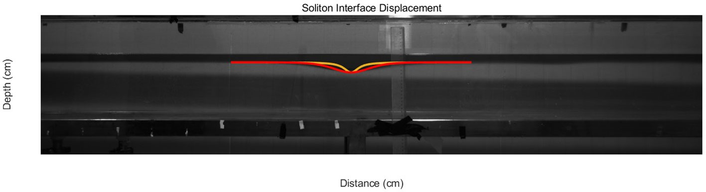
Figure 3. Wave shapes predicted by the KdV (red) and BO (yellow) models in comparison with the experimental wave shape.

The phase speed was also compared to further confirm the suitability of the KdV equation to model the specific mechanisms that this paper aims to shine a light on. Table 1 summarizes the linear phase speeds as well as the phase speeds observed experimentally, through the KdV equation, and the BO equation. It was clear that while $c_{KdV}$ fell within the acceptable range of $c_{experiment}$, $c_{BO}$ exceeded the upper limit in Experiment 1. Despite the fact that both $c_{KdV}$ and $c_{BO}$ were consistent with $c_{experiment}$ in Experiment 2, $c_{KdV}$ was closer to $c_{experiment}$.

Table 1

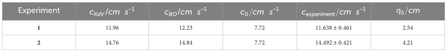
Table 1. Phase speeds and the corresponding errors in Experiments 1 and 2.

Thus, this paper draws the conclusion that the KdV equation is more efficacious for the cases we investigated. It produced more accurate results and was therefore more suitable than the BO equation, supporting the use of the KdV model and its extension, the vKdV model, with strong evidence.

3.2 Ice sheet

With the parameters described in the Materials and methods and the corresponding KdV internal solitary wave as the initial condition, simulations were produced using a pseudo-spectral method and fourth-order Runge-Kutta for the time-discretization at six positions (Figure 1B), which are (a) before the wave encounters the ice sheet, (b) immediately after it encounters it, (c) under the middle of the ice sheet, (d) immediately before it leaves, (e) immediately after it leaves, and (f) after it leaves. Relevant coefficients are shown in Figure 4. To compare the simulated wave shape with the experimental shape, the dye attenuation function in DigiFlow was used to interpret the experimental data.

Figure 4

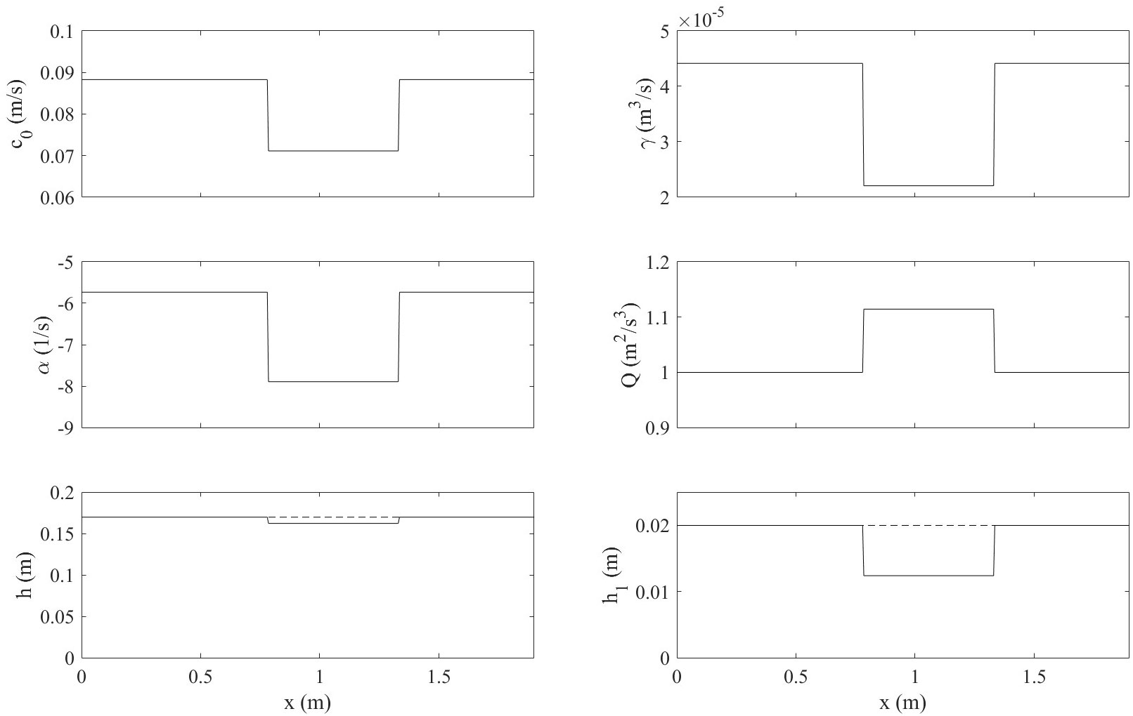
Figure 4. Coefficients in the vKdV equation applied to Experiments 3 and 4.

According to the simulation, in Experiment 3 (Figure 5), at (a), the internal solitary wave is the same as when it is first generated. Immediately after the wave encounters the sharp right-angled vertex of the ice sheet, at (b), it bent inwards at its back, first flatter, then steeper, and for this reason, the wave is slightly asymmetrical. As it reaches the middle of the ice sheet at (c), the bending disappears while an oscillation occurs behind the wave. The wave itself becomes thinner and taller, meaning a smaller half-width and a larger amplitude. During the evolution under the ice sheet, it continues to elongate, and at (d) the amplitude reaches its maximum. Immediately after the wave leaves the ice, a small twist appears at the end of the wave’s back. $18.0 cm$ further, the wave grew wider and shorter, with the oscillation it leaves behind significantly enhanced. An internal solitary wave with a larger initial amplitude (Figure 6) exhibits the same trend but more drastically. The bending at (b) is replaced by a wave-like train.

Figure 5

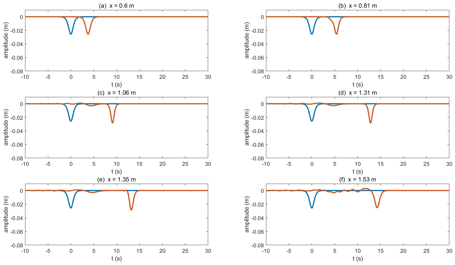
Figure 5. The vKdV simulation for Experiment 3. The blue line illustrates a reference wave at $t=0$ when the wave is generated. The red line traces the shape of the wave at positions (A-F).

Figure 6

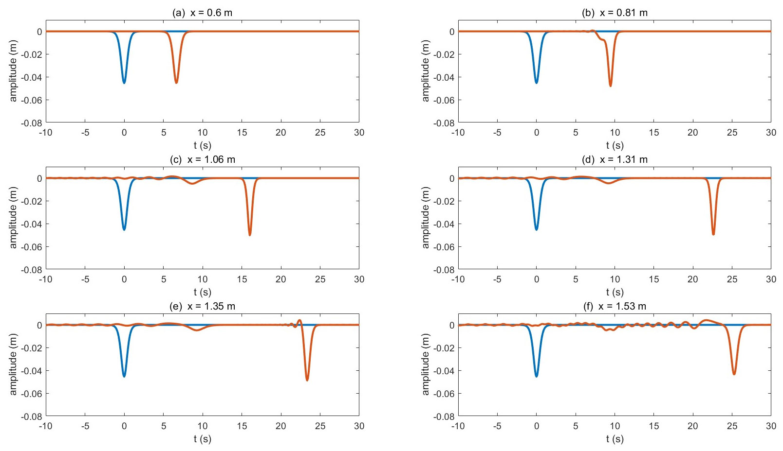
Figure 6. The vKdV simulation for Experiment 4 at the following locations: (A) before the wave encounters the ice sheet, (B) immediately after it encounters, (C) under the middle of the ice sheet, (D) immediately before it leaves, (E) immediately after it leaves, and (F) after it leaves. The blue wave is for reference, and the red wave is the evolutionary wave.

The vKdV model was used to collect amplitude predictions for every $2.5 cm$ increase in wave displacement in Experiment 3. A vKdV-amplitude graph was obtained and drawn onto the experimental amplitude graph (Figure 7). Both graphs exhibit similar wave amplitude trends: first increasing and then decreasing in response to the contact between the wave and the ice sheet. The amplitudes after the wave leaves the ice sheet are both lower than before the wave encountered the ice, indicating the possibility of either energy dissipation or the emission of very small linear waves. However, there are two differences: a) the vKdV model predicts a higher maximum amplitude than the experiment; b) the experiment suggests a surge followed by a plunge before the amplitude starts to climb towards its maximum. Ignoring the unexpected surge and plunge makes the experimental amplitude graph match with the vKdV graph effectively, as shown by the shifted experimental amplitude graph. The amplitudes begin to rise at similar locations, and adding back the overall decrease in the experimental amplitude caused by the increase and decrease raises the maximum amplitude to the proximity of the maximum vKdV-simulated amplitude. In other words, there is a $16 cm$ shift to the left required for the experimental result to match the trend of the simulation.

Figure 7

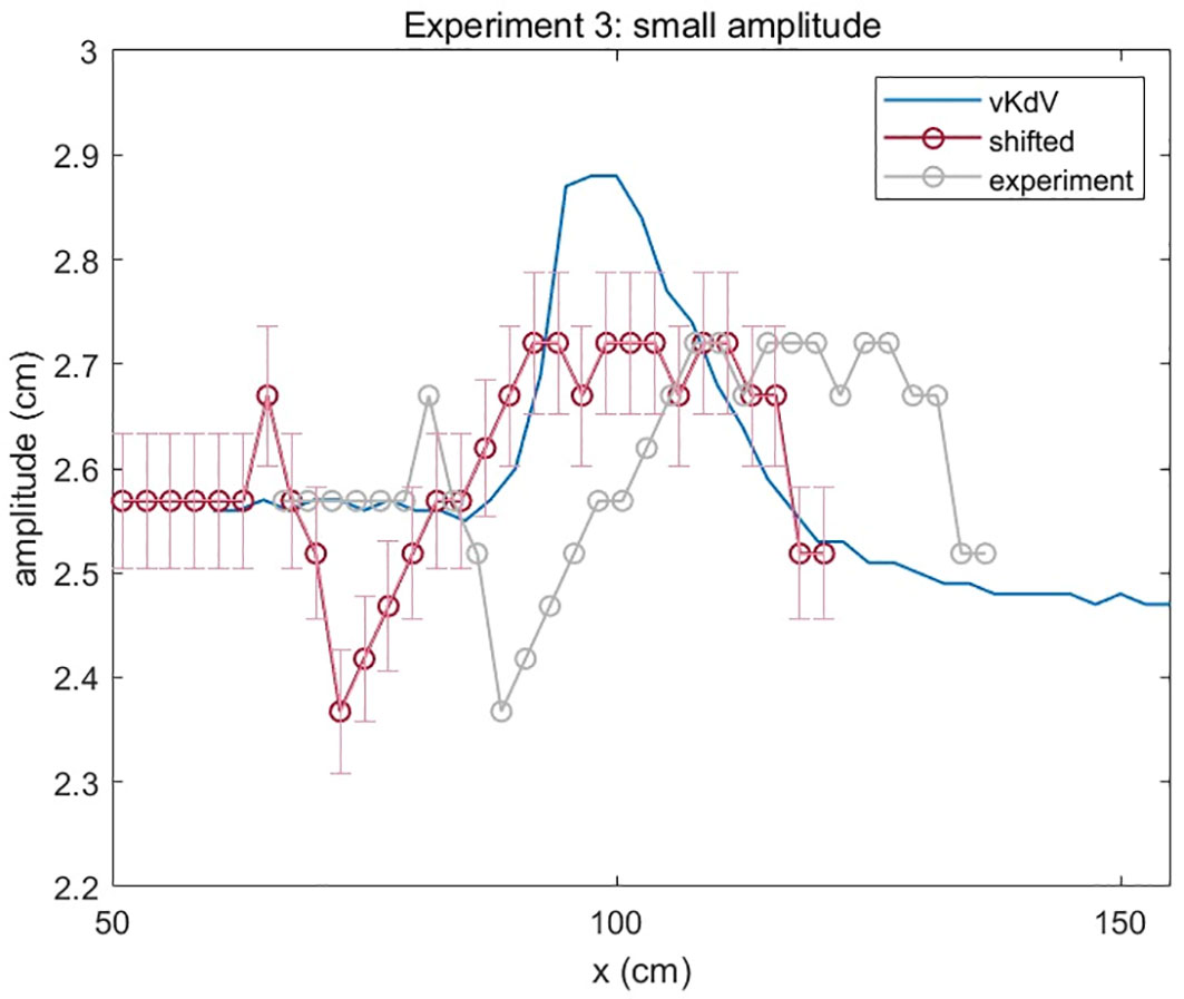
Figure 7. This graph depicts the change in the vKdV-predicted amplitude over horizontal displacement of the small amplitude wave in Experiment 3 due to the presence of the ice sheet. The development of experimental amplitude is also presented, as well as the shifting $16 cm$ leftwards.

The observed amplitude was also compared with the amplitude according to the asymptotic theory in Equation 13 in Grimshaw (2016). This theory states the relationship between amplitude a and α as follows:

$\begin{array}{ll}\begin{array}{c}\frac{a^3}{\alpha }=constant\end{array},& (36)\end{array}$

which is $a\propto {\alpha }^{\frac{1}{3}}$. In this case, α in Figure 4 shows consistency with the overall trend observed experimentally of first increasing and then decreasing. The magnitude of α increases to its maximum instantaneously when the wave meets the ice, and the (shifted) observed amplitude rises as well but less rapidly, although the vKdV-simulated amplitude rises at an even more gradual rate. When the wave leaves, the magnitude of α drops back to its initial value immediately. The (shifted) observed amplitude and vKdV amplitude follow, again, gradually.

To underscore the progression of the experimental wave, images from Experiment 4 were used, which detail more intense impacts from the ice sheet. In Figure 8, seven laboratory images of the wave at regular intervals portray the changes the wave has undergone. In the beginning, the wave does not appear to be much influenced, when comparing (a) and (b), before the wave arrives at the ice sheet and when only the front is under the ice. When a major part of the wave is below the ice in (c), the crest becomes less pronounced, leading to a trapezium wave shape. The crest soon recovers under the ice in (d), where the wave returns to a smooth rounded curve. The back expands while the front grows steeper, leaving a long tail after the asymmetrical wave, which seems to have evolved into oscillation. In (e) before the front of the wave exits the ice-covered water, the asymmetricity weakens. The front is longer, and an inward curve replaces the rather straight line at the back in (d), making it similar to the simulations illustrated in Figures 5B and 6B. During the period in which the wave leaves, in (f), the phenomenon that appeared in (e) is preserved. When the ice sheet is no longer above the wave in (g), the wave widens, assuming a less pointed form.

Figure 8

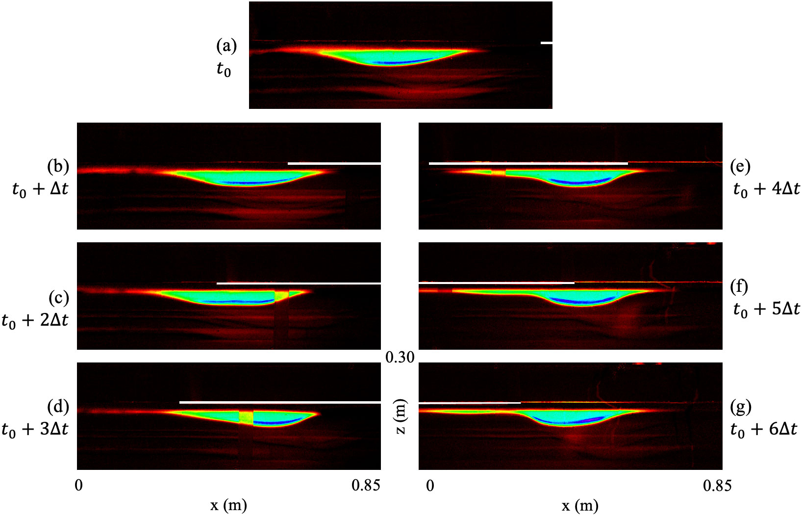
Figure 8. Wave evolution under the ice sheet in Experiment 4 over time. (A) The initial wave before the front of the wave reaches the ice sheet; (B) the wave $\text{Δ}t=1.33 s$ after (A); (C) the wave Δt after (B); (D) Δt after (C); (E) Δt after (D); (F) Δt after (E); (G) Δt after (F), right after the wave leaves the ice sheet. A reference ruler is set against the flume during the experiment, therefore, there is a rectangular vague yellowish area in (C–E). The ice is the white-colored shape.

The wave shape conveys the same shift as seen in the amplitude (Figure 7). The experimental wave shape after the majority of the wave overcomes the abrupt vertex of the ice edge (Figure 8C) disagrees with the predicted wave shape (Figure 9). The wave in the laboratory becomes flat at this position, forming a corner-rounded trapezium. Moreover, it does not seem to have that much oscillation at the back, as in Figure 9. Nevertheless, the simulation aligns with the experiment $16 cm$ after this moment. The distortion of the predicted wave shape corresponds well to the experimental in Figure 9 with a similar amplitude and a comparable prolongation at the end.

Figure 9

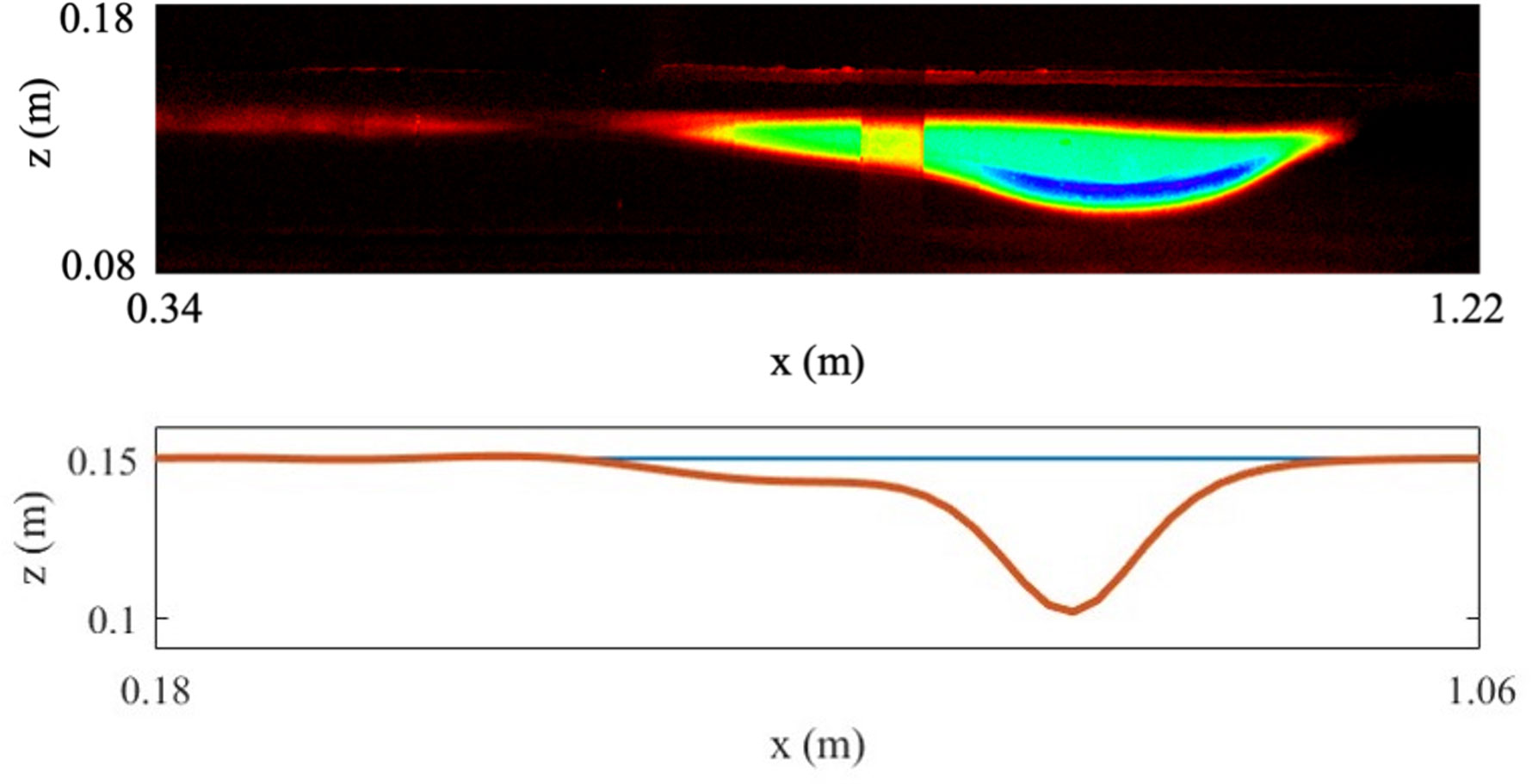
Figure 9. In the upper panel is the experiment image interpreted using the dye attenuation function in DigiFlow displaying the wave shape $16 cm$ after the simulation. The vague yellowish area close to the center is due to the reference ruler. In the lower panel is the simulated wave shape right after most of the wave starts to propagate under the ice sheet.

3.3 Ice keel

When the ice sheet was replaced with the ice keel in Experiment 5, the vKdV model provided a prediction for internal solitary waves with a pseudo-spectral method and fourth-order Runge-Kutta for the time-discretization at the following eight positions (Figure 1C): (a) before the wave arrives at the ice keel, (b) immediately after the wave meets the ice keel, (c) between the left end and the lowest point of the ice keel, (d) at the lowest point of the ice keel, (e) between the right end and the lowest point, (f) immediately before it leaves the ice keel, (g) immediately after it leaves, and (h) after it leaves. Figure 10 presents the corresponding coefficients involved in the simulation. Same as before, the dye attenuation function in DigiFlow is utilized on the experimental images.

Figure 10

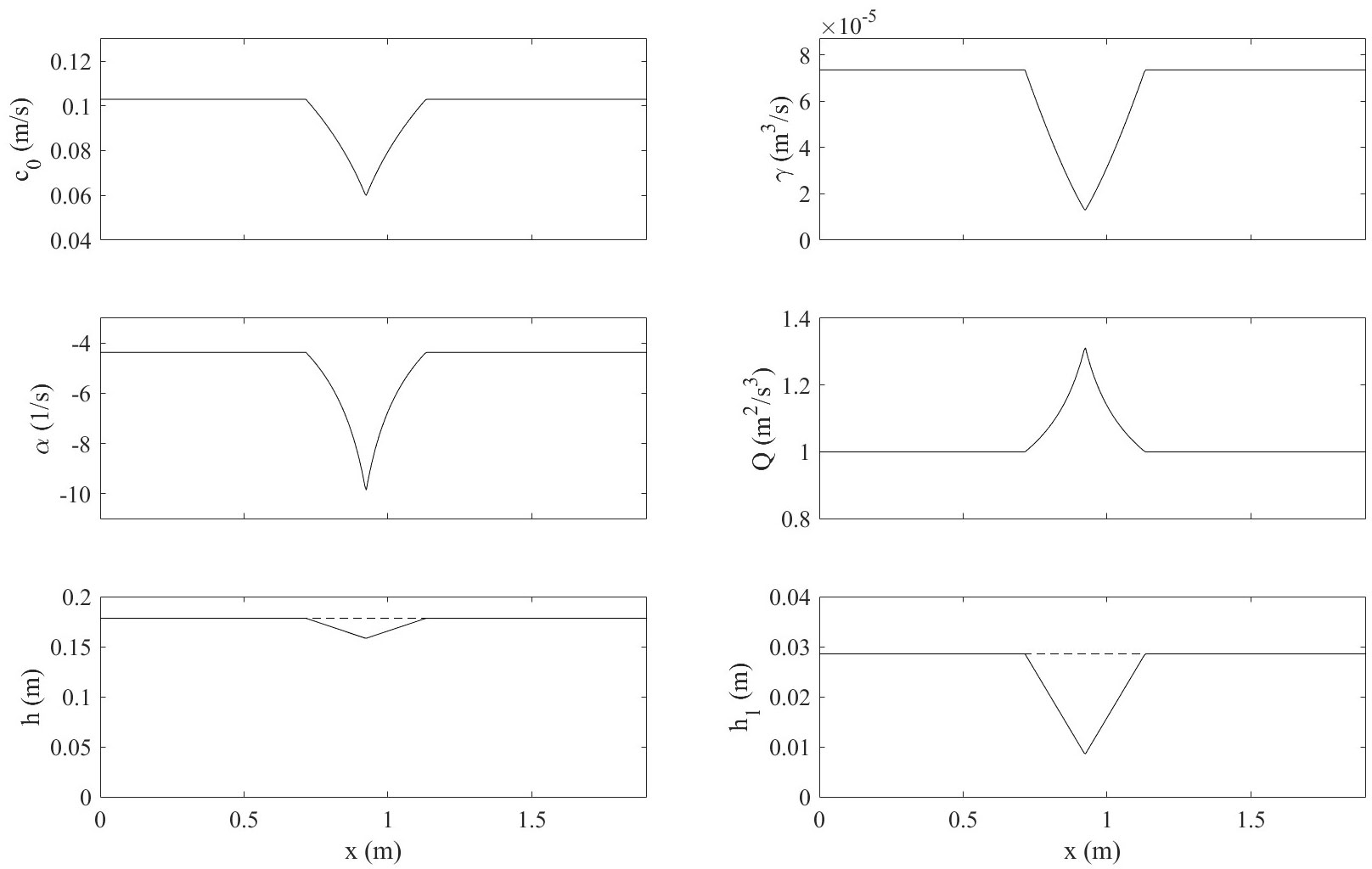
Figure 10. Coefficients in the vKdV equation applied to Experiment 5.

A simulation using the vKdV model (Figure 11) shows a little impact by the slight angle at the left vertex of the ice keel when the wave meets the ice at (b) compared to (a). Influenced by the downward slope of the ice at (c), an inward bending larger than that under the ice sheet occurs, and the wave is thus notably longer. The bending enlarges and eventually reaches the interface at (d), resulting in a linear sinusoidal internal wave radiating from the rear. The latter is substantially broader and more level, and the former is thinner and taller. Note that the process of the front wave is similar to the evolution under the ice sheet. Between (d) and (e) where there is an upward slope, the front wave shortens and widens, and the back wave deforms, with the crest collapsing inward and an increasing front space (i.e., between the two waves) pointing into the upper layer. Oscillation starts to appear behind the wave. In fact, the back wave begins to seem like part of the oscillation. Before leaving the ice keel at (f), the phenomenon persists. After the ice, at (g), the amplitude and shape of the front wave are almost identical to those at the beginning, yet the oscillation continues to amplify behind the wave. $19.5 cm$ further at (h), the wave is wider and shallower, and the oscillation is more vibrant, forming a sinusoidal shape where it connects to the wave.

Figure 11

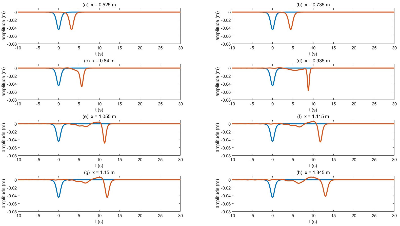
Figure 11. The vKdV simulation for Experiment 5 at the following locations: (A) before the wave arrives at the ice keel, (B) immediately after the wave meets the ice keel, (C) between the left end and the lowest point of the ice keel, (D) at the lowest point of the ice keel, (E) between the right end and the lowest point, (F) immediately before it leaves the ice keel, (G) immediately after it leaves, and (H) after it leaves. The blue wave at t = 0 is a reference wave. The red shows the transformation of the studied wave.

Laboratory images of Experiment 5 are presented in Figure 12. When the wave first encounters the ice keel, the simulation is very consistent with the experiment. During this period, the wave travels from the ice edge to the bottom of the ice, inward bending takes place at the back of the wave as predicted despite being less significant than expected. Even so, since the majority of the wave has passed the vertex at the bottom, it diverges from the simulation and the wave is deformed by the vertex and broadened. Also, there seem to be traces of it separating into two waves as indicated by the two “lumps”. One piece of evidence is the blue line near the bottom of the wave in Figure 12E. Nonetheless, the wave is not actually divided into two, and the second half of the wave (the left “lump”) is not shortened or flattened as predicted. From (e) to (g), the second “lump” shrinks and appears to be part of the oscillation created by the vertex at the bottom. After the wave leaves the ice [(g) and (h)], the oscillation is very thin but long, elongating along the interface more than ever. The connection between the wave and the oscillation weakens, suggesting the possibility of an emerging space as predicted by simulation. The wave in (h) is larger than in (g), at which the wave has diminished a little due to the “lump” spreading out as oscillation, but still, the wave in (h) is substantially smaller than it initially is in (a). While vKdV simulation successfully forecasts the oscillation, the details of the oscillation differ from the experiment.

Figure 12

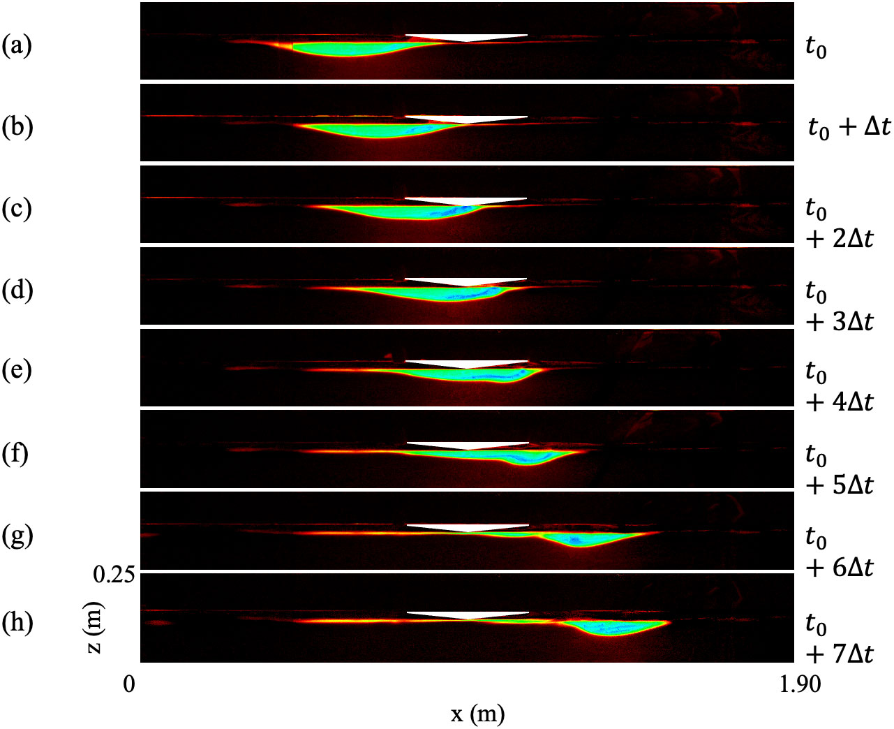
Figure 12. Wave transformation under the ice keel over time in Experiment 5. (A) The wave when the front of the wave touches the ice keel; (B) the wave $\text{Δ}t=0.80 s$ after (A); (C) the wave Δt after (B); (D) Δt after (C); (E) Δt after (D); (F) Δt after (E); (G) Δt after (F); (H) Δt after (G) right after the wave leaves the ice keel. The ice is the white-colored shape.

Note that at the time the wave has mostly left the ice and almost only the oscillation is still below the ice, the major wave shape fits with the predicted model much better than at the previous stages, in spite of the predicted uprisen interface following the major wave not being recognized (Figure 13). The wave shape appears to have recovered from the trough of the ice, better matching the simulation than when the wave propagates from the ice trough to the ice edge.

Figure 13

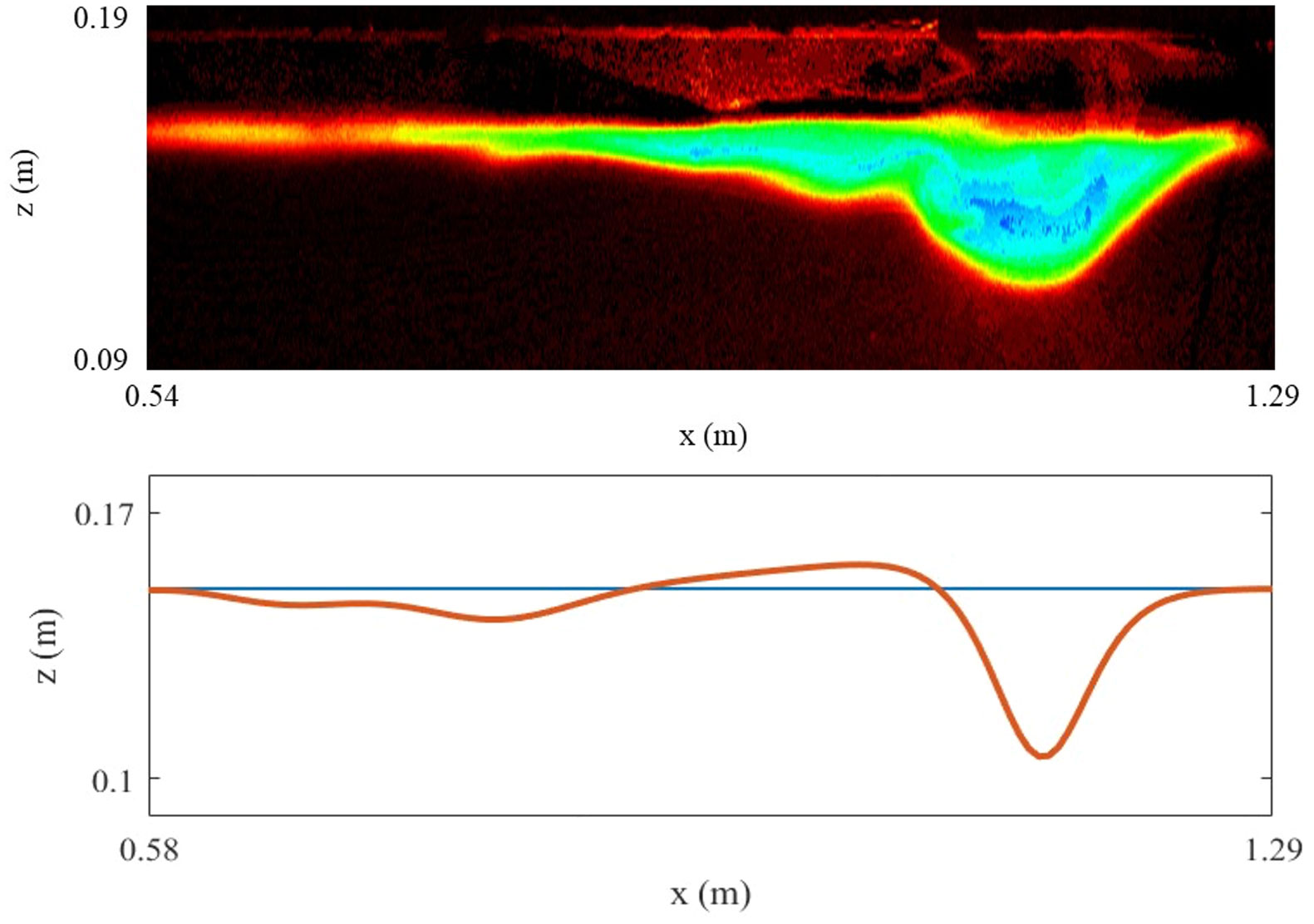
Figure 13. In the upper panel is the experiment image interpreted using the dye attenuation function in DigiFlow which outlines the wave at $1.15 m$ when the majority is out of the ice-keel-covered water. In the lower panel is the simulated wave shape at $1.15 m$, the same position as in the upper panel.

4 Discussion

Since the KdV model was developed, it has continued to attract interest, and while it seemed to be a model particularly for weakly nonlinear waves in shallow water (weak nonlinearity defined as $\frac{\eta }{h_{eff}}\ll 1$; shallow water defined as $\frac{\lambda }{h}\gg 1$), it has been applied to large amplitude non-shallow solitary waves which violate the assumptions mentioned above for its “robust range of validity” (Grue et al., 1999; Koop and Butler, 1981; Michallet and Barthelemy, 1998; Segur and Hammack, 1982; Small et al., 1999; Helfrich and Melville, 2006). Several laboratory findings from Ostrovsky and Stepanyants (2005), Koop and Butler (1981), and Segur and Hammack (1982) point out that even in deep water, KdV still demonstrates good correlation with observations, better than BO, a model designed for deep water conditions. However, some field observations argue for the opposite. For example, Wang and Pawlowicz (2011) found that BO predictions align with observations made in the deep water of the Strait of Georgia far better than KdV. After all, the comparison between KdV and BO in this paper supports the former. Despite being claimed to have almost the broadest application among all models and equations, the reason for this suitability remains speculative (Small et al., 1999).

The ice sheet and ice keel imposed similar effects on the internal solitary waves but to a different extent. Oscillation and deformation occurred due to the vertices of the ice. There was a reduction in amplitude in all the sea ice experiments after the internal solitary wave left the ice compared to the beginning, possibly implying energy dissipation or the emission of very small, unobservable linear waves. The wave amplitude surged and then plunged in the first encounter of the ice sheet. The right angle at the vertex caused the wave to form a trapezium shape with rounded corners, yet the crest reformed afterward. The amplitude increased to its maximum and then decreased to lower than initially it was, during which the wave developed an asymmetrical shape but soon lost it. It left the ice sheet with a rather regular shape, although smaller and round-bottomed. For the ice keel, inward bending was seen when the wave was under the downward slope. The bottom vertex of the ice keel induced the potential formation of a second wave, indicated by two “lumps”, which flattened along the way and became an oscillation. The wave looked rather regular but was significantly smaller after it left the ice keel, with a tail at its back.

The vKdV model offers overall good agreement with the experimental observations, yet there are occasions when the simulation is inconsistent with laboratory results. The $16 cm$ shift that arose in Experiment 3 (Figures 8, 10) was the same as the shift in Experiment 4, indicating that they could be caused by the same reason. With regards to the corresponding vKdV coefficients in Figure 4, the sharp right-angled vertices of the ice sheet are probably the cause, as the vKdV model is more effective for situations where the coefficients are slowly changing. The vKdV model predicted the later evolution but less sufficiently considered the effects of the vertices, which led to the shift that occurred in both experiments. Such a vertex is a singular point, where the derivative of $h_1(x)$ does not exist. Hence the vKdV is not suitable here. The same happened for Experiment 5, where instead of a right angle, there was an obtuse angle at the vertex, which was, still, a singular point. Compared to the vKdV models’ performance in Experiments 3 and 4, the influence of the obtuse angle was smaller, possibly due to the fact that the vertex was flatter, and the angle was the only one large enough to be effective. Nonetheless, thanks to Roger Grimshaw for pointing out that vKdV can be used when coefficients are slightly discontinuous, caused by, for example, a slight change in depth, assuming there is no wave reflection and the equation holds before and after (personal communication, July 2024).

Nevertheless, while the sharp vertices violate vKdV’s slow variation assumption, regardless of the effects of the angles, the vKdV model provides generally adequate simulations for further research. It indicated an accurate reduction in amplitude after the ice and an appropriate maximum (Figure 7), depicted good wave shapes after the shift, and suggested a creditable overall trend in Experiment 3. A noteworthy point is that in the experiments the effects of ice appear to share similarities with a variable topography, and some were also seen in the vKdV simulations. As suggested by Knickerbocker and Newell (1980), when an internal solitary wave propagates along a varying topography, the wave deforms with elevated waves developing. Likewise, while the vKdV simulations in this paper did not fully report the observed results or such results, waves of elevation and deformation did occur.

Moreover, this study speculates that for cases where the stratification is not two-layered (e.g., continuous stratification), the vKdV model remains useful. As asserted by Grimshaw (2016), the KdV model can serve as a fundamental framework for modeling oceanic internal solitary waves. Numerical simulations are growing more popular for scenarios with variable topography and hydrology to be considered, despite computational limits. Regarding the full nonlinearity of the internal solitary waves in the experiments in this paper, vKdV simulations combined with numerical simulations using models such as MITgcm are worth looking at.

Data availability statement

The datasets analyzed for this study can be found in the Experimental and Theoretical Studies of Sea Ice Effects on Internal Solitary Waves_data.zip. Link: https://figshare.com/articles/dataset/Frontiers_data_zip/27022417?file=49198852.

Author contributions

JT: Conceptualization, Data curation, Formal analysis, Investigation, Methodology, Software, Validation, Visualization, Writing – original draft, Writing – review & editing.

Funding

The author(s) declare that no financial support was received for the research, authorship, and/or publication of this article.

Acknowledgments

I would like to express my deepest gratitude to Professor Roger Grimshaw at University College London for guiding me throughout the research and writing process. Without his guidance, this paper would not be possible. I would also like to thank Yaoren Zhang, Shiqiang Hu, and Xiudan Ruan for assisting with ice making and the experimental setup, and discussions about the vKdV model. I sincerely appreciate all constructive comments and suggestions from the reviewers, which helped us to improve the quality of the manuscript.

Conflict of interest

The author declares that the research was conducted in the absence of any commercial or financial relationships that could be construed as a potential conflict of interest.

Publisher’s note

All claims expressed in this article are solely those of the authors and do not necessarily represent those of their affiliated organizations, or those of the publisher, the editors and the reviewers. Any product that may be evaluated in this article, or claim that may be made by its manufacturer, is not guaranteed or endorsed by the publisher.

References

Benjamin T. B. (1966). Internal waves of finite amplitude and permanent form. J. Fluid Mech. 25, 241–270. doi: 10.1017/S0022112066001630

Crossref Full Text | Google Scholar

Bernstein R. L. (1972). Observations of currents in the Arctic Ocean. Palisades, N.Y: Lamont-Doherty GeologicalObservatory of Columbia University.

Google Scholar

Bernstein R. L., Hunkins K. (1971). Inertial currents from a three-dimensional array in the Arctic Ocean. Eos Trans. AGU 52, 255.

Google Scholar

Carr M., Sutherland P., Haase A., Evers K. U., Fer I., Jensen A., et al. (2019). Laboratory experiments on internal solitary waves in ice-covered waters. Geophys. Res. Lett. 46, 230–212. doi: 10.1029/2019GL084710

Crossref Full Text | Google Scholar

Czipott P. V., Levine M. D., Paulson C. A., Menemenlis D., Farmer D. M., Williams R. G. (1991). Ice flexure forced by internal wave packets in the Arctic Ocean. Science 254, 832–835. doi: 10.1126/science.254.5033.832

PubMed Abstract | Crossref Full Text | Google Scholar

D’Asaro E. A., Morison J. H. (1992). Internal waves and mixing in the Arctic Ocean. Deep Sea Res. Part II 39, S459–S484. doi: 10.1016/S0198-0149(06)80016-6

Crossref Full Text | Google Scholar

Ekman V. W. (1904). “On dead water,” in Norwegian North Polar Expedition 1893–1896 (Longmans, Green and Co), 1–150.

Google Scholar

Fer I. (2014). Near-inertial mixing in the central Arctic Ocean. J. Physi. Oceanogr. 44, 2031–2049. doi: 10.1175/JPO-D-13-0133.1

Crossref Full Text | Google Scholar

Garrett C., Munk W. (1972). Space-time scales of internal waves: A progress report. J. Geophys. Res. 80, 291–297. doi: 10.1029/JC080i003p00291

Crossref Full Text | Google Scholar

Grimshaw R. (1981). Evolution equations for long nonlinear internal waves in stratified shear flows. Stud. Appl. Math. 65, 159–188. doi: 10.1002/sapm1981652159

Crossref Full Text | Google Scholar

Grimshaw R. (2016). Nonlinear wave equations for oceanic internal solitary waves. Stud. Appl. Math. 136, 214–237. doi: 10.1111/sapm.12100

Crossref Full Text | Google Scholar

Grimshaw R. (2024). Personal communication (London, United Kingdom: University College London).

Google Scholar

Grue J., Jensen A., Rusas P., Sveen J. (1999). Properties of large-amplitude internal waves. J. Fluid Mech. 380, 257–278. doi: 10.1017/S0022112098003528

Crossref Full Text | Google Scholar

Hartharn-Evans S. G., Carr M., Stastna M. (2024). Interactions between internal solitary waves and sea ice. J. Geophys. Res.: Oceans 129, e2023JC020175. doi: 10.1029/2023JC020175

Crossref Full Text | Google Scholar

Helfrich K., Melville W. (2006). Long nonlinear internal waves. Ann. Rev. Fluid Mech. 38, 395–425. doi: 10.1146/annurev.fluid.38.050304.092129

Crossref Full Text | Google Scholar

Kirillov S. (2006). Spatial variations in sea-ice formation-onset in the Laptev Sea as a consequence of the vertical heat fluxes caused by internal waves overturning. Polarforschung 79, 119–123. Available online at: http://epic.awi.de/28582/1/Polarforsch2006_3_4.pdf.

Google Scholar

Knickerbocker C. J., Newell A. C. (1980). Internal solitary waves near a turning point. Phys. Lett. 75, 326–330. doi: 10.1016/0375-9601(80)90830-0

Crossref Full Text | Google Scholar

Koop C. G., Butler G. (1981). An investigation of internal solitary waves in a two-fluid system. J. Fluid Mech. 112, 225–251. doi: 10.1017/S0022112081000372

Crossref Full Text | Google Scholar

Levine M. D., Paulson C. A., Morison J. H. (1985). Internal waves in the Arctic Ocean: Comparison with lower-latitude observations. J. Phys. Oceanogr. 15, 800–809. doi: 10.1175/1520-0485(1985)015<0800:IWITAO>2.0.CO;2

Crossref Full Text | Google Scholar

Liu Z., Grimshaw R., Johnson E. (2017). Internal solitary waves propagating through variable background hydrology and currents. Ocean Modelling 116, 134–145. doi: 10.1016/j.ocemod.2017.06.008

Crossref Full Text | Google Scholar

Liu Z., Grimshaw R., Johnson E. (2018). The effect of a variable background density stratification and current on oceanic internal solitary waves. MDPI Fluids. 3, 96. doi: 10.3390/fluids3040096

Crossref Full Text | Google Scholar

Marchenko A. V., Morozov E. G., Muzylev S. V., Shestov A. S. (2010). Interaction of short internal waves with the ice cover in an Arctic fjord. Oceanology 50, 18–27. doi: 10.1134/S0001437010010029

Crossref Full Text | Google Scholar

Michallet H., Barthelemy E. (1998). Experimental study of interfacial solitary waves. J. Fluid Mech. 366, 159–177. doi: 10.1017/S002211209800127X

Crossref Full Text | Google Scholar

Morison J. H. (1986). “Internal waves in the Arctic Ocean: A review,” in Geophysics of Sea Ice. Ed. Untersteiner N. (Plenum, New York: Springer New York, NY).

Google Scholar

Morison J., Long C. M., Levine M. L. (1985). Internal wave dissipation under sea ice. J. Geophy. Res. 90, 959–911. doi: 10.1029/JC090iC06p11959

Crossref Full Text | Google Scholar

Muench R. D., LeBlond P. H., Hachmesiter L. E. (1983). On some possible interactions between internal waves and sea ice in the marginal ice zone. J. Geophys. Res. 88, 2819–2816. doi: 10.1029/JC088iC05p02819

Crossref Full Text | Google Scholar

Munk W. H. (1981). “Internal waves and small-scale processes,” in Evolution of physical oceanography (Cambridge, Massachusetts: MIT press).

Google Scholar

Nansen F. (1902). The Norwegian North Polar Expedition 1893-1896: Scientific Results (Vol. 3) (Longmans, Green and Co).

Google Scholar

Neshyba S. J., Neal V. T., Denner W. W. (1972). Spectra of internal waves: In situ measurements in a multiple-layered structure. J. Phys. Oceanogr. 2, 91–95. doi: 10.1175/1520-0485(1972)002<0091:SOIWSM>2.0.CO;2

Crossref Full Text | Google Scholar

Ono H. (1975). Algebraic solitary waves in stratified fluids, J. Phys. Soc Japan 39, 1082–1091. doi: 10.1143/JPSJ.39.1082

Crossref Full Text | Google Scholar

Osborne A. R., Burch T. L. (1980). Internal solitons in the Andaman Sea. Science 208, 451–460. doi: 10.1126/science.208.4443.451

PubMed Abstract | Crossref Full Text | Google Scholar

Ostrovsky L. A., Stepanyants A. (2005). Internal solitons in laboratory experiments: comparison with theoretical models. Chaos 15, 1–28. doi: 10.1063/1.2107087

Crossref Full Text | Google Scholar

Saiki R., Mitsudera H. (2016). A mechanism of ice-band pattern formation caused by resonant interaction between sea ice and internal waves: A theory. J. Physi. Oceanogr. 46, 583–600. doi: 10.1175/JPO-D-14-0162.1

Crossref Full Text | Google Scholar

Sandven S., Johannessen O. M. (1987). High-frequency internal wave observations in the marginal ice zone. J. Geophys. Res. 92, 6911. doi: 10.1029/JC092iC07p06911

Crossref Full Text | Google Scholar

Segur H., Hammack J. L. (1982). Soliton models of long internal waves. J. Fluid Mech. 118, 285–304. doi: 10.1017/S0022112082001086

Crossref Full Text | Google Scholar

Small J., Hallock Z., Pavey G., Scott J. (1999). Observations of large amplitude internal waves at the Malin shelf-edge during SESAME 1995. Cont. Shelf Res. 19, 1389–1436. doi: 10.1016/S0278-4343(99)00023-0

Crossref Full Text | Google Scholar

Stokes G. G. (1847). On the theory of oscillatory waves. Camb. Trans. 8, 441–473.

Google Scholar

Sutherland B., Dauxois T., Peacock T. (2014). “Internal waves in laboratory experiments,” in Modeling Atmospheric and Oceanic Flows 1^st ed. Eds. von Larcher T., Williams P. D. (American Geophysical Union and John Wiley & Sons, Inc, New Jersey USA), 193–212. doi: 10.1002/9781118856024.ch10

Crossref Full Text | Google Scholar

Wang C. (2009). Geophysical observations of nonlinear internal solitary-like waves in the Strait of Georgia. (Doctoral dissertation). University of British Columbia, Vancouver. doi: 10.14288/1.0053118

Crossref Full Text | Google Scholar

Wang C., Pawlowicz R. (2011). Propagation speeds of strongly nonlinear near-surface internal waves in the Strait of Georgia. J. Geophys. Res. 116, C10021. doi: 10.1029/2010JC006776

Crossref Full Text | Google Scholar

Wunsch C. (1976). Geographical variability of the internal wave field: a search for sources and sinks. J. Phys. Oceanogr. 6, 471–485. doi: 10.1175/1520-0485(1976)006<0471:GVOTIW>2.0.CO;2

Crossref Full Text | Google Scholar

Yearsley J. R. (1966). Internal waves in the Arctic Ocean, M.S. thesis, Mech. Eng. Dept., University of Washington, Seattle.

Google Scholar

Zhou X., Grimshaw R. (1989). The effect of variable currents on internal solitary waves. Dyn. Atmos. Oceans 14, 17–39. doi: 10.1016/0377-0265(89)90055-9

Crossref Full Text | Google Scholar