Acoustic tags versus camera—a case study on feeding behaviour of European seabass in sea cages

Intoduction: With the expansion of the aquaculture industry, the need arises for scalable, reliable, and robust methods to assess fish behaviour in sea cages to guide operational management, which includes feeding optimisation and welfare assessments. Fish cage monitoring utilising either acoustic transmitters or underwater cameras is well-studied. However, the relationship between those two different measurement types seems to have not been explored, nor have they been evaluated together in one experimental site.

Methods: In our 1-month study, we compared the activity of 14 sentinel fish and the artificial intelligence (AI)-inferred speed of individuals from the European seabass (Dicentrarchus labrax) sea cage population in three feeding trials. Comparisons include a maximum activity comparison using persistent peaks, fish behavioural pattern establishment and retention, and periodical behavioural patterns.

Results: Our results demonstrate that under certain circumstances, both technologies are interchangeable from the perspective of persistent peaks and periodicity, but complementary when it comes to behaviour analysis such as food anticipatory behaviour (FAB).

Discussion: We anticipate that our findings will stimulate advances where multiple sensor types are in use to achieve a more holistic understanding of fish behaviour in the aquaculture sector using underwater technologies.

1 Introduction

In recent years, the aquaculture sector has been increasing its production output rapidly (FAO, 2024; Verdegem et al., 2023) with more or larger locations that require oversight. It is therefore almost a necessity to be able to have remote or autonomous control to optimise farm practices such as feeding; not just to reduce feed waste and maximise growth, but also to be aware of early fish welfare issues. Camera systems (Al-Jubouri et al., 2018; Georgopoulou et al., 2024), hydroacoustics (Orduna et al., 2021; Samedy et al., 2015), and acoustic telemetry (Chen et al., 2023; Føre et al., 2018; Kolarevic et al., 2016) are known tools for fish monitoring purposes in aquaculture. Yet, all three technologies deliver only a partial view on the fish stock in an aquaculture installation, since for camera and hydroacoustic sensors, the focal view might not represent the population correctly, while in acoustic telemetry, though offering continuous monitoring, only few fish individuals can be tracked at the same time.

In this case study, we compare the acceleration data from acoustic telemetry with the readings of a camera system that uses artificial intelligence (AI) to monitor fish speed in an attempt to extract fish behaviour patterns and to qualify the camera-based approach.

All in all, we aim to contribute to automated fish behaviour analysis through the assessment of movement (i.e., acceleration and speed) as accurate categorisation of fish behaviour can guide operational procedures such as feeding management by optimising feeding times.

1.1 Tracking fish with acoustic telemetry

Acoustic telemetry utilises sound that attenuates slower in water and has a higher range than in air (Jacoby and Piper, 2023). Typical setups include an array of acoustic receivers, which can be spread out over the area of interest, and acoustic transmitters that are either implanted or tagged onto individual fish (Wagner et al., 2011; Leroy et al., 2023). This type of setup has been useful in tracking the migration of wild fish populations through widespread receiver arrays and tagging of fish individuals (Lédée et al., 2021).

In aquaculture, studied species of commercial interest include Atlantic salmon (Salmo salar) (Kolarevic et al., 2016; Stockwell et al., 2021) or the European seabass (Dicentrarchus labrax) (Alfonso et al., 2022; Georgopoulou et al., 2022, 2024) and the monitoring parameters are often similar: Depending on the transmitter sensors, metrics such as activity, depth, angle, temperature, salinity, and many others can be used to interpret moving patterns. The data collection itself happens through acoustic receivers that take in data-encoded sound waves sent by the transmitters. Depending on the manufacturer and setup, systems provide either manual data-fetching after or during trials by recovering the receivers, or real-time communication possibilities for immediate data access. In both cases, the acoustic telemetry data can provide in-depth behaviour qualification of the tagged individuals or be used for welfare assessments (Alfonso et al., 2022; Carbonara et al., 2021).

1.2 Tracking fish with camera systems

In recent years, the utilisation of computer vision techniques in aquaculture has emerged as a powerful tool for monitoring and understanding fish behaviour without the need for invasive or lethal methods (Georgopoulou et al., 2024; Zhou et al., 2018b; Han et al., 2020; Wang et al., 2021; Yang et al., 2021b). These methods range from infrared imaging for tracking fish and studying feeding behaviour (Pautsina et al., 2015; Zhou et al., 2017) to stereo cameras for fish detection and individual tracking (Torisawa et al., 2011; Chuang et al., 2015). Notably, single-camera systems utilising visible spectrum cameras have demonstrated efficacy in detecting fish, classifying behaviour, and tracking fish across various aquaculture systems, including recirculating aquaculture systems (RAS) (Liu et al., 2014; Kong et al., 2022) and sea cages (Foster et al., 1995; Hu et al., 2022; Ubina et al., 2021; Pradana and Horio, 2022). Moreover, the development of intelligent monitoring and control methods, leveraging mathematical models and machine learning algorithms, has further enhanced the capability to extract meaningful insights from captured data.

As technology advances, more sophisticated techniques, such as deep learning, have been integrated into these methodologies, offering automated and non-invasive means of recording behavioural parameters (Macaulay et al., 2021a). The process typically involves converting images into statistical data using computer vision models, enabling the estimation of behavioural parameters ranging from swimming speed and direction to spatial distribution and feeding activity (Yang et al., 2021a). Other studies offer a thorough investigation and discussion on computer vision techniques used for monitoring fish behaviour (An et al., 2021; Li et al., 2020; Niu et al., 2018; Wang et al., 2021; Yang et al., 2021b; Zhou et al., 2018a).

Regarding feeding, studies applying computer vision and AI for fish feeding monitoring have primarily focused on RAS with controlled environments. Early approaches used traditional computer vision, such as analysing frame differences to measure feeding activity (Liu et al., 2014) or combining vision with machine learning to assess fish behaviour (AlZubi et al., 2016). More advanced methods employed convolutional neural networks (CNNs) for classifying feeding-related activities (Han et al., 2020; Kong et al., 2022) and multi-task CNNs for active/inactive classification (Wang et al., 2022). In sea cages, fewer studies exist, often relying on indirect appetite measures like feed loss detection (Hu et al., 2021) or surface activity monitoring (Ubina et al., 2021). A notable effort combined 3D-CNNs and RNNs to capture spatiotemporal information of the behaviours in salmon (Måløy et al., 2019).

1.3 Main contribution

Studies have and are exploring the application scope, advantages, and limitations of acoustic telemetry (Macaulay et al., 2021b; Li et al., 2024a) and camera systems (Li et al., 2024b; Saberioon et al., 2017) in aquaculture settings. Since both technologies operate on different output data, and their “field of view” on aquaculture installations are inherently different, the question arises whether cameras and tags can deliver the same or comparable behavioural output parameters.

Even if we assume that both technologies do deliver useful behavioural output parameters when used in conjunction, uncertainties remain. Academic literature is, to the best of our knowledge, not informative on whether shifting from acoustic telemetry using acceleration to camera systems using fish movement speed or vice versa can be conducted without loss of underlying behavioural patterns. Additionally, it is unclear if monitored fish behaviour can be translated from one sensor type to the other, and if so, whether the corresponding monitored fish behaviour is equally pronounced or if there are other effects (e.g., delay effects) at play. Lastly, the same underlying behavioural pattern could be exhibited entirely differently depending on the sensor type, possibly showing complementary instead of similar patterns. Since acoustic telemetry can deliver continuous monitoring, one might be interested in qualifying fish behaviour results from camera systems with it. Yet, no study to our knowledge has conducted direct comparisons of acoustic telemetry and a camera system in the same experiment.

The research question therefore is whether cameras can be qualified by acoustic transmitters for fish behaviour in sea cages, opening the avenue for potential interchangeability.

We focused our comparisons on different feeding behaviour frameworks, as we expect pre-occurring food anticipation behaviour and periodical patterns to be interchangeably or complementarily being detected across measurement type.

Altogether, we were interested in three main key comparisons:

Comparison of peaks. In order to discuss the (dis-)similarities between the peak values between activity and speed throughout different feeding trials, we identified the so-called persistent peaks. We focused on the three highest persistent peaks per 24-h day, which we would map against the closest feeding time to find out if there are potential differences in the peak distribution between activity and speed. Additionally, it was of interest to see if there are peak distribution changes within one measurement type across the experiment phases.

Comparison of temporal properties. We aimed to find out if the periodicity of daily patterns would be similar between activity and speed, even though there are no speed data for the night time due to lack of light. For that purpose, we calculated the periodicity with the autocorrelation function (ACF) of the time series for activity and speed for each experiment phase, respectively, to observe potential differences.

Comparison of pattern establishment and retainment. Concerning pattern establishments, we aimed to explore whether the data readings for the first and second feeding would synchronise around the respective feeding time in the feeding phases with two feedings per day, regardless of measurement type. Furthermore, it was of interest if increases in locomotion are caught by both measurement types, and how strongly food anticipatory behaviour (FAB) would be expressed.

2 Material and methods

2.1 Experimental design

The data considered in this study ranged from 02 June 2023 00:00 to 12 July 2023 23:59 local time (UTC+3).

2.1.1 Experimental animals and site

A group of more than 10,000 European seabass (D. labrax, 450 ± 30 g body weight) at a stocking density of 7.8 kg/m³ was reared in a circular polyester cage (perimeter, 40 m; depth, 9 m) having a cylinder-shaped net down to 8 m depth and a closing cone of 1 m. The sea cage was located on the pilot farm of HCMR. The stock was obtained from the Mesocosm hatchery of HCMR. After the larval rearing period and the pre-growing stages at 120 days post-hatching, juveniles of 2 g mean weight were transferred to the pilot scale farm.

2.1.2 Automatic feeder

An automatic feeder was located at the centre of the cage. It comprised a microcomputer (rpi, Raspberry Pi 4 Model B) that was used as a node that controlled a simple motor (feeding motor, 12V). To enable remote control of the feeder, the MQTT communication protocol (messaging protocol for the transmission of data from sensors) was used. During the trial, the feeder was activated at specific times (see below) and for a specific duration according to the experimental protocol as explained below.

2.1.3 Feeding times

Feeding practices in the Mediterranean aquaculture do not apply a unified feeding protocol as feeding regimes can vary from one time daily feeding to continuous feeding, but feeding events themselves usually occur during light hours only. Feeding time also seems to serve as an external synchronizer for feeding processes and digestion (Samori, 2024).

Consequently, locomotor activity related to feeding is being influenced by the application of different feeding regimes, as we see for fish movement speed in Georgopoulou et al. (2024). Considering the fish’s dual foraging capabilities (Martins et al., 2012) and the limited information available on the impact of different feeding protocols on behaviour around feeding such as food anticipatory activity (FAA), we aimed to test our systems at different feeding times to determine whether these variations affect FAA and how this is reflected through both camera observations and acoustic tags. Changing feeding regimes might also reveal more beneficial feeding strategies as there is no single precise strategy that takes into consideration all welfare aspects for the farmed fish (López-Olmeda et al., 2012).

The total feeding duration per feeding day was 30 min, and the amount of feed (Zoonomi S.A., Gorgo 6 mm) was modified according to temperature and was at 0.5% of the total biomass. When there were two feedings per day, each feeding session lasted 15 min with equal feed quantities. The experiment was split up into different phases with fasting periods in-between, as shown in Table 1. During the experimental period, the operation of the feeder was not normal for some days and the relevant data were not used in the analysis. These days were designated as “Irregular Phases”. Note that we differentiated feeding and non-feeding windows with the feeding times provided in Table 1, independent of other data input.

Table 1

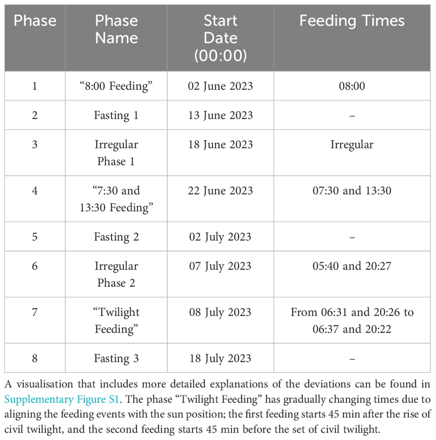
Table 1. The experimental setup of the feeding times.

2.2 Tracking fish activity with acoustic telemetry

Fifteen acoustic transmitters (ADT-LP7, Thelma Biotel Ltd.) and three receivers (TBR700, Thelma Biotel Ltd.) were used for the experiment. The transmitters were equipped with a three-axis accelerometer that converted the raw acceleration to m/s² and then filters out static components like gravity. Over the sampling duration, the root mean square (RMS) value was calculated, which was then transmitted by the tags. Additionally, the transmitters were equipped with pressure sensors for depth and temperature sensors. The setup and location of the tags and receivers were almost identical to the trial of Chen et al. (2023), with some minor differences. The receivers were submerged at the edges of the sea cage in a triangle at a depth of 2.5 m, but no additional synchronisation tag (R-HP16, Thelma Biotel Ltd.) was added to the system.

The temperature resolution was 0.1°C and the activity had a resolution of 0.013588 m/s² and a range of 0 to 3.465 m/s². A modification of the setup in Chen et al. (2023) was that the depth signal registration interval was every 30 to 50 s (mean, 40 s), and accordingly, the doubled interval for temperature or activity (mean, 80 s), since temperature and activity values were sent alternating in addition to depth data.

2.2.1 Transmitter implantation

The whole implantation protocol follows the same schemata as described in Georgopoulou et al. (2022) and short-lined in Chen et al. (2023). We state here the outline of the procedure: On 21 April 2023, 25 fish of 37.07 ± 180 cm total length and 582.05 ± 187.83 g weight were transferred from the pilot scale farm to a 10-m³ tank at HCMR facilities (T = 18°C, pH = 8.0, salinity = 36 psu, DO > 5 mg/L, and ambient photoperiod). On 03 May 2023, fish were sedated, and the acoustic transmitters [Thelma Biotel Ltd., 7.3 mm diameter, 23.2 mm length, 1.8 g weight in water, and less than 2% tag-to-body-weight ratio (Jepsen et al., 2005)] were transplanted into the peritoneal cavity of 15 randomly chosen individuals, which were afterwards transferred into a 5-m³ tank for recovery (Georgopoulou et al., 2022). The tag activation was on 02 May 2023 and the sea cage transfer was on 23 May 2023.

2.2.2 Transmitter data collection and processing

Data pre-processing followed a similar pipeline as in Chen et al. (2023) with the only major change being that the no GPS positions were calculated and that the bandwidth for signal-to-noise ratio (SNR) was changed to [20,inf). The pipeline in short consisted of the following steps:

Raw data were downloaded and processed using the software ComPort (Thelma Biotel, v4.0.3) from the three receivers around the sea cage. Each extracted data point from a tag had an entry for depth and, alternately, an entry for temperature and activity. We decoded the entries to create time series for depth, activity, and temperature, respectively. The time series for depth, temperature, and activity have then been mean-resampled on a resolution of 10 min.

Finally, missing values (k_activity= 10, k_depth= 8, k_temperature= 9) were filled by linear interpolation, leading to 144 × 41 = 5,904 data points, respectively (number of 10-min intervals per day × experiment days). Note that the interpolation of values was for methodology alignment between the two measurement types.

2.3 Tracking fish speed with underwater camera

2.3.1 Camera setup

Recordings were made using a Fyssalis V3.1 camera (Element S.A., Greece) capturing at 10 fps and with an image resolution of 1,280 × 720 pixels. Data at night could not be recorded since visibility was insufficient. The “breaking” point between sensible detections against dark images for the camera analysis was around 6:00 for the morning and 21:00 in the evening; therefore, those times were picked as a hard cutoff, resulting in 15 h worth of data per 24-h day.

2.3.2 Calculating speed of fish

The videos were analysed using a previously developed system based on YOLOv5 and deepsort (Georgopoulou et al., 2024). The speed in frame i was calculated as

$\begin{array}{ll}{u}_i=\sqrt{{(x(i)-x(i-1))}^2+{(y(i)-y(i-1))}^2}& (1)\end{array}$

where x and y are the coordinates of the fish.

To minimise noise and extreme speed values, we chose fish that were consecutively tracked for a minimum of five frames and applied the Savitzky–Golay filter (window s_w = 5, polynomial order s_p = 2) on the centres of the fish. The unit of measurement for speed was bd/s. The speed values were then binned in 10-min intervals, and for missing values between 6:00 and 21:00, a linear interpolation was conducted (k_speed = 393). The total number of these 10-min bin data points for the experiments was n_speed = 6 × 15 × 41 = 3,690 (10-min intervals per hour × hours considered per day × experiment days).

2.4 Using persistent homology to detect peaks

In order to capture relative height in the complicated nature of the time series for activity and speed in our fish experiment (see Figure 1), we used a tool set called topological data analysis (TDA) with pioneering work of Edelsbrunner et al. (2002) to locate peaks in time series. Persistent homology (PH) (Edelsbrunner et al., 2002; Edelsbrunner and Harer, 2008) is one of the tools that encompasses the study of mathematical features like holes and components.

Figure 1

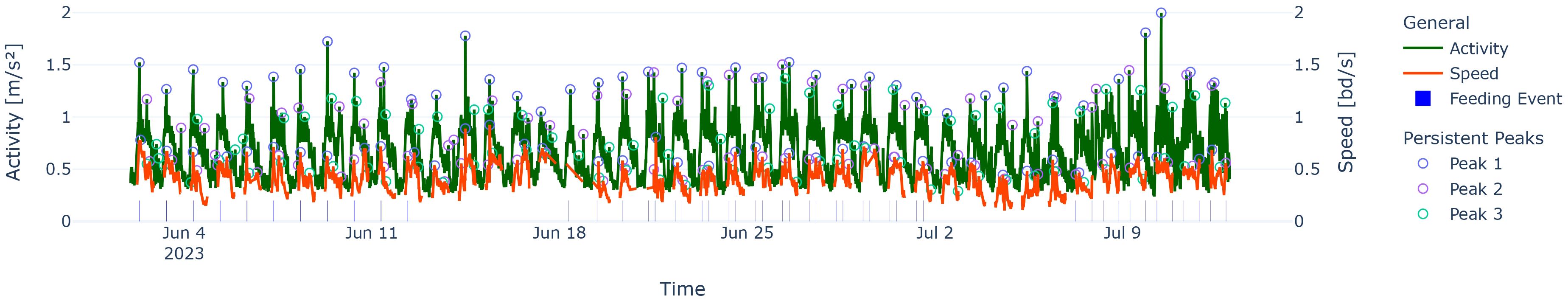
Figure 1. Activity and speed over the experiment period marked with persistent peaks of different rank (circles) and feeding events (vertical strips above the x-axis). Note that the width of the feeding event follows the time axis; therefore, the stripes can be visually challenging to see.

As the specific method was not the focus of this paper, we present it in a descriptive way in Section 2.4.1. We refer to the proper mathematical literature for the unsatisfied reader when it comes to relevant properties and their proofs as well as the computation for higher dimensions (Malott et al., 2023; Munch, 2017; Chazal and Michel, 2021; Fugacci et al., 2016; Edelsbrunner and Harer, 2008).

One of the desired properties was the noise resistance, as time series for both activity and speed tend to fluctuate, even after binning into 10-min intervals. For persistent peaks, if we added noise up to ϵ to all data points, the resulting persistent peak calculation would only differ by 2ϵ at most (Cohen-Steiner et al., 2007; Huber, 2021). Conversely, only relying on the n highest absolute points on each 24-h day might have led to misleading results, as we exemplified in Figure 2.

Figure 2

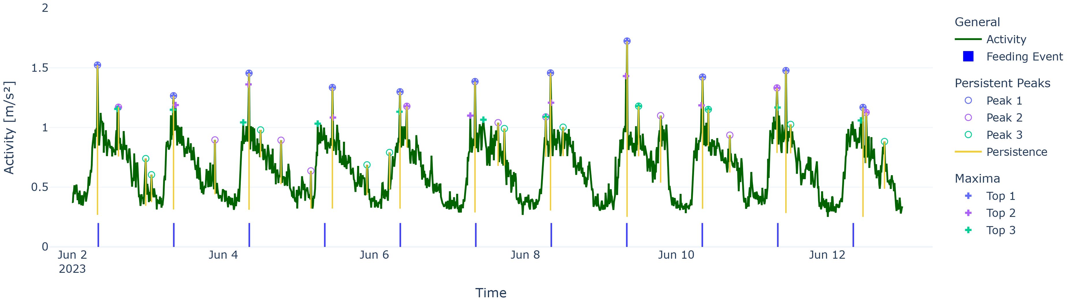
Figure 2. Comparison of using persistent peaks (circles) vs. maxima by value (crosses), exemplified in phase “8:00 feeding”. Note that maxima top 2 and top 3 have a tendency to cluster around the feeding time, while Peak 2 and Peak 3 tend to spread.

We adapted the method from Huber (2017) to extract the n_peaks = 3 most significant peaks for each day for activity and speed, respectively (see Figures 1, 2). We call those peaks “Peak n” or “Persistent Peak of rank n”, respectively.

2.4.1 From a flood to mountain tops

We describe the algorithm used for Figures 1 and 2 visually after Huber (2017) where the mountain tops are local maxima and a mountain range is a 24-h day: Imagine a time series ${(a_i)}_{i\in \{1,\dots ,n\}}$ for some n ∈ ℕ to be a mountain range that is cut vertically. Now, consider a receding flood above the highest mountain top as a perfect horizontal line.

We track appearing mountain tops by marking their highest point and drawing a vertical line downwards following the water level. The essence of persistence peaks is knowing when to stop drawing the line. When two mountains are connected through the lowering water level, we stop drawing the line for the lower mountain. We stop drawing the line for the highest mountain the moment the whole mountain range is connected. This line segment will naturally have the value $\text{max}({(a_i)}_{i\in \{1,\dots ,n\}})-\text{min}({(a_i)}_{i\in \{1,\dots ,n\}})$ with n ∈ ℕ being the number of data points in the time series.

The length of each vertical line is the persistence of the respective mountain top point. The three mountain tops with the highest persistence are selected as persistent peaks of rank 1/2/3. In all brevity, the chosen persistent peaks mathematically corresponds to the selection of the three most persistent 0th-dimensional cycles when looking at the superlevel set filtration of the time series ${(a_i)}_{i\in \{1,\dots ,n\}}$ (Huber, 2017). Thereby, a persistent peak A in ${(a_i)}_{i\in \{1,\dots ,n\}}$ has the (absolute) height h_A and the persistence p_A as an indicator for relative height. We say that persistent peak A is “higher” than another persistent peak B when its persistence value is higher (p_A > p_B). An illustration of the method for two persistent peaks is given through a time series with four points in Figures 3A–E. In PH, one can also encode the “start” (birth) and the “end” (death) of the persistence of persistent peaks in a so-called “persistent diagram”, which we display for completeness sake in Figure 3F.

Figure 3

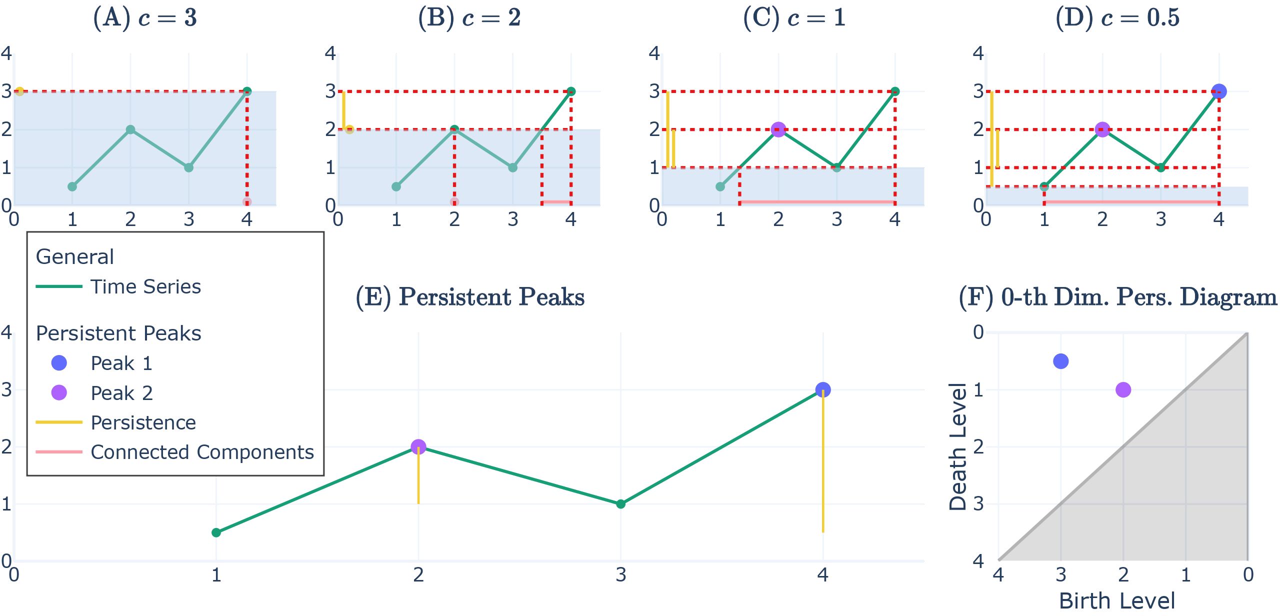
Figure 3. Time series ${(a_i)}_{i\in \{1\dots 4\}}$ with receding with water level c, persistent peak of rank 1 and 2, and persistent diagram D₀. (A–D) Visualisation of receding water levels c to mark persistent peaks and track their persistence as mountain ranges (connected components) are merging. The light blue area visualises the receding water level mentioned as the flood in Section 2.4.1. (E) The time series with persistent peak of rank 1 and 2 where the persistence is marked (yellow). (F) The corresponding 0th-dimensional persistence diagram D₀ to the graph in (E). It illustrates an alternative way to show the “lifetime” of persistent peaks by mapping the water level at which the persistent peak’s mountain starts onto the x-axis as “birth level” and the water level where the persistent peak’s mountain range merges as “death level”; therefore, persistence = birth level − death level.

2.5 Food anticipatory behaviour detection

To measure anticipatory behaviour, FAA as in Azzaydi et al. (2007) was considered. For the detection of sudden but then sustained high-activity windows, similar to Chen et al. (2023) and Azzaydi et al. (2007), the length and intensity were key parameters: The acceleration activity threshold follows the setup protocol as in Chen et al. (2023) and was thereby set at the 0.5 quantile, while the movement speed threshold was derived naively by enforcing that also 12 h worth of data points would lie over the threshold, which led to a (15 h – 12 h)/15 h = 0.2 quantile.

It has been shown that the swimming speed of the European seabass is significantly lower during nocturnal hours than during diurnal hours in a similar floating pen setup (Neo et al., 2018). We therefore conducted the analysis under the assumption that these results translate into our experiment setup to a degree when making the choice for the quantile threshold for speed.

The minimum duration criterion of the high fish activity was set to 60 min, respectively. We locked the FAA detection until 2 h post-feeding to account for elevated movement and general activity during that time.

2.6 Statistical methods

Kruskal–Wallis tests were used to compare activity and speed, respectively, across neighbouring phases (irregular phases excluded beforehand) of the experiment for each persistent peak rank. To compare activity and speed regarding how close their respective highest persistent peaks were to the feeding schedule, we calculated the time difference between the persistent peaks and the closest feeding time (or the feeding time of the previous phase for the fasting phases), respectively. Afterwards, Kruskal–Wallis tests were used for each section and persistent peak rank to identify alterations in the time difference to the closest feeding time, as the differences were not normally distributed.

The ACF for the activity and speed time series for each experiment phase was calculated to evaluate the periodicity patterns. We calculated the highest correlated interval using the starting point P0 and the highest points in the following “hill” of the graph where values are positive, and marked that point as P1. Afterwards, the time interval between them was calculated. Note that for activity, 24 h correspond to 144 lags (as we have a time resolution of 10 min and 6 × 24 = 144), but that for speed, a 24-h cycle corresponds to only 90 lags (since we cut off times outside of the time interval 6:00–21:00, leaving us with 15 h and therefore 6 × 15 = 90 lags).

Augmented Dickey–Fuller (ADF) unit root tests and Kwiatkowski–Phillips–Schmidt–Shin (KPSS) tests were used on the activity, speed, depth, and temperature time series for the experiment window, respectively, to test for stationarity.

To evaluate whether classical FAA was first detected for activity or speed, proportion z-tests were conducted. Likewise, the test was used to identify whether activity or speed was retained longer after the feeding period.

Dependent t-test for paired samples was used to test if the average depth around the feeding times was different in the phases with two feeding times.

Unless otherwise stated, a p-value smaller than 0.05 was considered significant. All statistical analyses was conducted in Python v.3.8. For exact reproducibility, links to the code and data can be found under the data availability statement.

3 Results

Sensor data from 14 out of 15 fish individuals were used for analysis. The remaining tag was believed to be malfunctioning or damaged (data suggested it was floating on top of the sea cage).

3.1 Persistent peaks analysis

3.1.1 Statistical analysis

When comparing the activity and speed peaks independent from each other across non-irregular neighbouring experiment phases, there were, with one exception, no significant differences in the time difference to the closest feeding (Kruskal–Wallis test, p ≥ 0.05, respectively). The exception was a time difference in hours for speed between the phase “Fasting 1” and “7:30 and 13:30 Feeding” for persistent peaks of rank 1 (Kruskal–Wallis test, H = 4.8167, df = 1, p < 0.05), as marked in Figure 4.

Figure 4

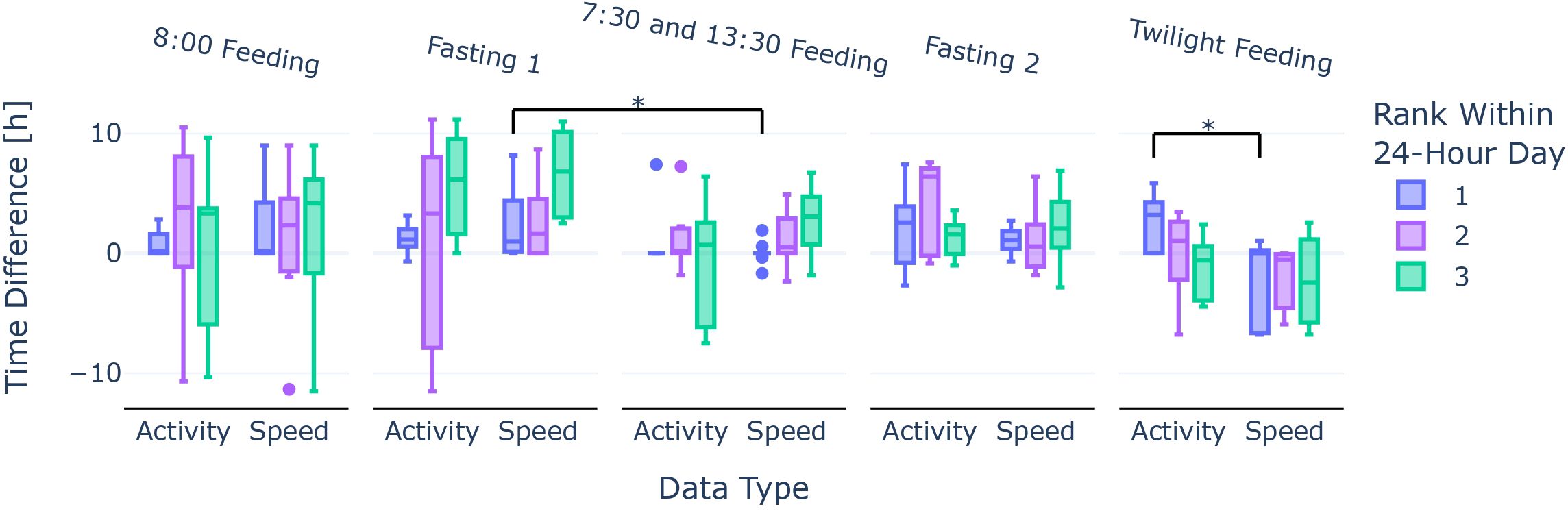
Figure 4. Time difference in hours of the three highest persistent peaks for activity and speed towards the feeding time or the last applicable feeding time from the previous phase. The bars are colour-coded: Peaks of rank 1 are blue, peaks of rank 2 are violet, and peaks of rank 3 are green. Each central box represents the interquartile range (IQR = Q3−Q1) with the median (Q2) marked as a line, and whiskers are positioned at 1.5 times the IQR away from the central box edges. The asterisk (*) marks a significance difference between groups (Kruskal–Wallis test, p < 0.05).

When comparing the two data types for each section and persistent peak rank within a 24-h day, respectively, activity and speed were not significantly different (Kruskal–Wallis test, p ≥ 0.05 respectively), except for the phase “Twilight Feeding” for persistent peaks of rank 1 (Kruskal–Wallis test, H = 4.036, df = 1, p < 0.05), as marked in Figure 4.

Exhaustive tables for the Kruskal–Wallis tests can be found in Supplementary Tables S1, S2.

3.1.2 Dispersion during fasting

A dispersion trend of the feeding pattern was observed for activity in the phases Fasting 1 and Fasting 2 as the boxes and whiskers widened or moved compared to the previous feeding phases, respectively. In particular, the Peak 1 bar for Fasting 1 and Peak 1 and Peak 2 bars for Fasting 2 show strong deviation from the previous feeding time(s) (see Figure 4).

When comparing the persistent peaks of rank 1 and 2 for speed between the Fasting 1 phase and the previous “8:00 Feeding” phase, the difference was not as striking as for activity, respectively. When comparing the “7:30 and 13:30 Feeding” phase with the following Fasting 2 phase, there was a dispersion of the Peak 1 bars (see blue Fasting 2 bars in Figure 4).

3.1.3 Lagging of dispersion

During the first feeding phase, for both activity and speed, we observed a trend where Peak 1 was lagging behind the feeding event at 8:00. Peak 2 and Peak 3 were spread out. The “Fasting 1” phase, on the other hand, showed a trend for the activity Peak 1 to be lagged behind, as seen by the detached box [interquartile range (IQR) between 0.58 and 2.04], and lagging speed persistent peaks (see Figure 4). Additionally, Peak 2 for activity had the highest variability in this phase (IQR of 15.92) for any Peak 2s throughout the experiment.

3.1.4 Focus during feeding

We observed a concentration of Peak 1s at the feeding times in the “8:00 Feeding” and the “7:30 and 13:30 Feeding” phase regardless of data type, as shown in diminishing bars in Figure 4, though the Peak 1s for speed in the “8:00 Feeding” were more spread than for activity.

Additionally, we found relatively small Peak 2 bars for the “7:30 and 13:30 Feeding” phase in Figure 4 (activity Peak 2 IQR: 2.08, speed Peak 2 IQR: 2.92) that stemmed from the Peak 2s often being on the alternate feeding event that was not occupied by the Peak 1 of the day (see Figure 5).

Figure 5

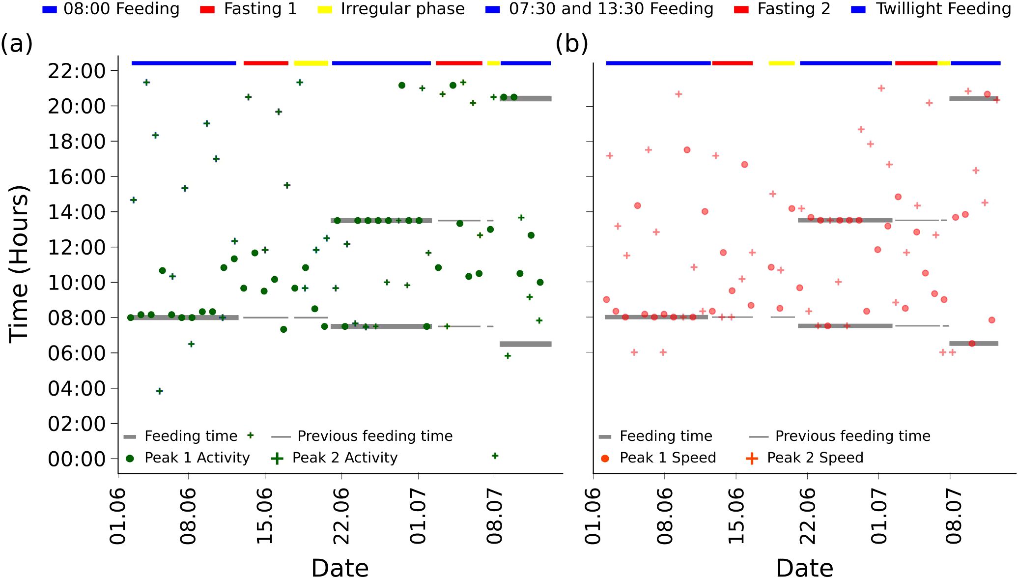
Figure 5. Scatter plot of Peak 1s (circles) and Peak 2s (crosses) for activity (A) and speed (B), for the different experiment phases (shown in different colours) and (reference) feeding times. Note that the gradual minute change of the feeding times between the days in the phase “Twilight Feeding” is not visible.

Furthermore, we observed that there was a concentration of persistent peaks of rank 1 at the only feeding event for the phase “8:00 Feeding”, but this changed when considering the phase “7:30 and 13:30 Feeding”, where the Peak 1s were concentrated around the noon feeding, regardless of data type (activity, speed) (see Figure 5).

Lastly, the phase “Twilight Feeding” seemed to be contradictory with the Peak 1 boxes for activity lagging behind the feeding time in Figure 4, but the Peak 1s and Peak 2s for speed seemed to be too early for the feeding. It should be noted that the number of data points for the phase “Twilight Feeding” was the smallest with N_days = 5 instead of N_days = 11 or N_days = 10 like in the other two feeding phases, respectively; therefore, more uncertainty was inherently given.

3.2 Periodicity insights

3.2.1 Periodicity

We observed a quite consistent 24-h periodic pattern in all ACF plots across measurement types (activity, speed) and experiment phases (see Figure 6). The shown periods in Figure 6 were calculated by subtracting P1 from P0 and were similar between activity and speed, though the deviations from 24 h for speed were higher with up to 0.53 h (ca. 32 min).

Figure 6

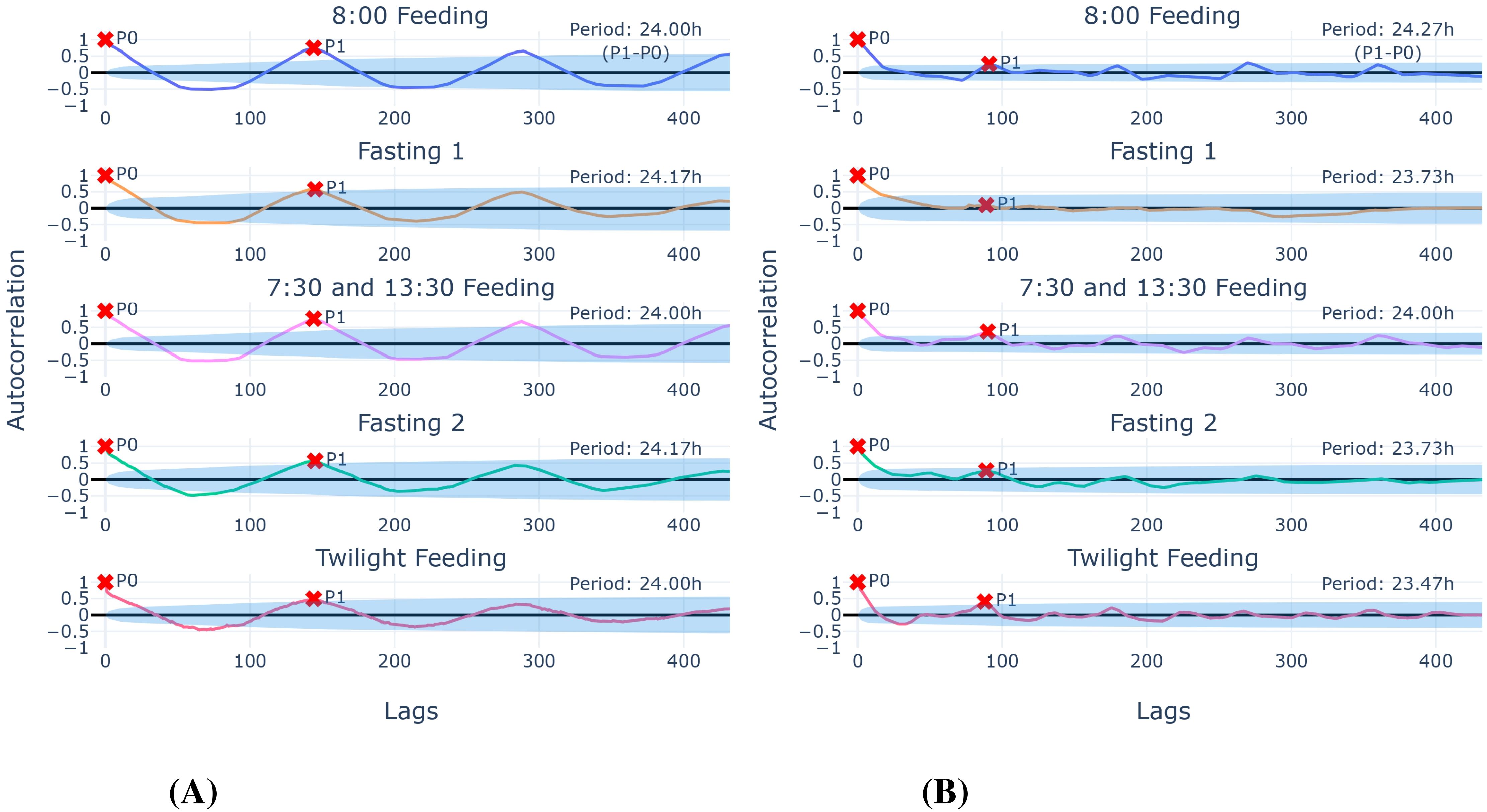
Figure 6. Autocorrelation function for activity (A) and speed (B) in the different experiment phases. The period is calculated by P1 − P0, where P0 and P1 are consecutive local maxima. Points lying outside the lying-cone shaped area around the x-axis (5% significance limits) are considered significant. One lag corresponds to 10 min for (A), and 16 min for (B) (since speed data points outside of the interval 6:00–21:00 were excluded).

Although all P1 autocorrelation values in Figure 6A were significant for activity, the autocorrelation values for the fasting phases [ρ(145) ≈ 0.58 and ρ(145) ≈ 0.56, respectively] and the twilight phase [ρ(144) ≈ 0.49] are just approximately 0.5, contrary to the first two feeding phases [ρ(144) ≈ 0.75 and ρ(144) ≈ 0.76].

Compared to the ACFs for the speed time series in Figure 6B, the fasting phases did not show a significant P1 (second local maxima), indicating the absence of a notable daily pattern during these periods.

Additionally, the wavelet power transform also showed the 24-h periodicity of the activity (see Figure 7). For fasting periods or pause periods, the pattern disappeared (the light areas became less pronounced).

Figure 7

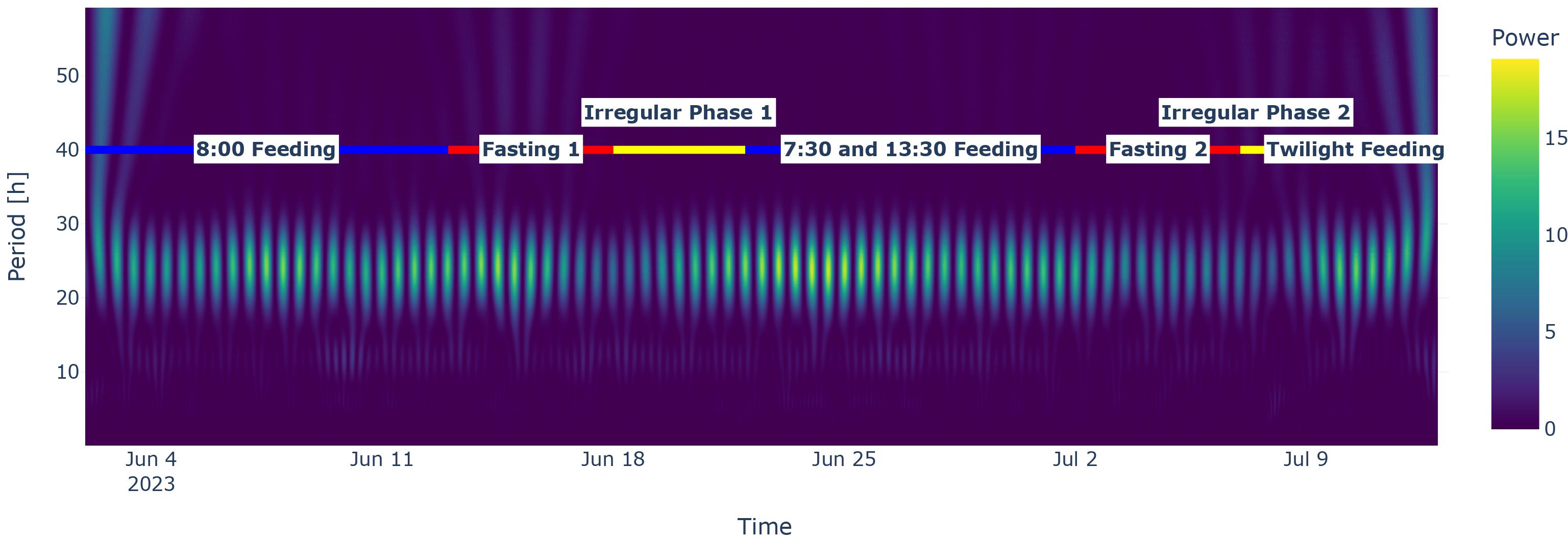
Figure 7. Wavelet spectrum for the activity time series. Note the stripes throughout the experiment feeding phases with the highest power at around 24 h. The coloured horizontal line represents the experiment phases. Blue indicates a feeding phase, red denotes a fasting phase, and yellow indicates an irregular phase.

However, the wavelet power transform for speed was not interpretable. Both without and with spline interpolation for the night (see Supplementary Figure S2), the speed periodicities were not clearly readable or were noisy when comparing with a priori knowledge about the experiment phases.

3.2.2 Correlation between activity and speed

When conducting a full cross-correlation between the activity time series and the speed time series, the highest significant coefficient was at zero lags, indicating that the best match was the Pearson correlation coefficient with ρ = 0.46. Furthermore, the shape of the cross-correlation function was asymmetric with a slower decrease for negative lags (see Supplementary Figure S3). As a lag was the frequency of the time series, the 24-h periods are different for activity and speed, where one 24-h day for activity corresponds to 144 lags, but 90 lags made up a 24-h day for speed (owing to the cutoff times for the speed time series, see Section 2.3.2).

3.3 Feeding patterns

3.3.1 Stationarity

For the experiment window, the depth and activity time series extracted from the transmitters and the speed time series were both stationary (ADF test, p < 0.05 and KPSS test, p > 0.05), allowing for more reliable downstream statistical analysis such as autocorrelation. However, the temperature time series was not stationary by the same tests. The significance of the test statistics on the speed time series with gaps (see Section 2.3.1) was invariant against first-order spline interpolation or filling the gaps with 0 values. Therefore, the different speed time series variants were also stationary (ADF test, p < 0.05 and KPSS test, p > 0.05, respectively).

3.3.2 Behaviour around feeding

For the phase “7:30 and 13:30 Feeding”, fish were significantly in deeper waters (0.68 ± 0.24 m) when feeding occurred at 13:30 than for the feeding at 7:30 (dependent t-test for paired samples, p < 0.05), as illustrated in Figure 8. For the phase “Twilight Feeding”, no significant difference was found (dependent t-test for paired samples, p ≥ 0.05).

Figure 8

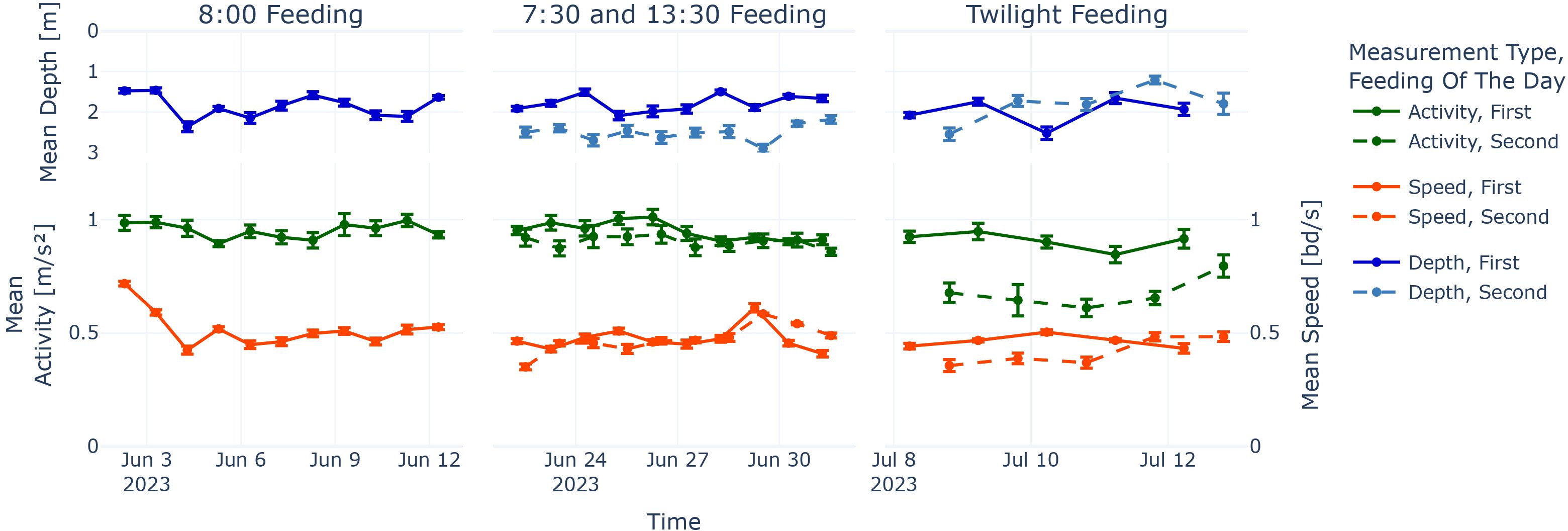
Figure 8. Activity, speed, and depth around feeding events. Values are means of activity, speed (green and orange line graphs), and depth (blue line graphs) ± SEM from 1 h before feeding until 2 h after feeding for each feeding event. All line graphs follow the continuous time x-axis; therefore, the first and second feeding are shown with offset where applicable.

When looking at the activity around feeding for the two phases with two feeding times, there was a significant difference between the first and second feeding, respectively (dependent t-test for paired samples, p < 0.05).

In a qualitative manner, it did seem like that the second feeding activity means were syncing up with the first feeding of the day; while being more or less below the first feeding activity mean at the beginning of the phases with two feedings, the difference disappears towards the end of the phases. Even though we had only a few days for the “Twilight Feeding”, one could see a trend of the activity means from the second feeding going up towards the means of the first feeding.

For the phases “7:30 and 13:30 Feeding” and “Twilight Feeding”, there was no significant difference in the speed around the first and the second feeding (dependent t-test for paired samples, p ≥ 0.05). We note that the speed data points around the first feeding in “7:30 and 13:30 Feeding” were not normally distributed (Shapiro–Wilk test, p < 0.05).

3.3.3 Food anticipatory and post-feeding behaviour

Activity was a reliable tracker for FAA for the feeding phases (see the green bottom stripes prior to feeding in Figure 9). The start of FAA for activity was significantly more often earlier than for speed (one proportion z-test, n = 51, p < 0.05). On the other hand, speed was significantly more often trailing behind than activity (one proportion z-test, n = 51, p < 0.05), meaning that even though activity levels have suspended, the speed levels are still within of high-value-window considerations. Both tests were invariant against the number of hours added to the feeding end to measure “true” post-feeding activity/speed (n_hours∈{0,1,2}), nor did it depend on the minimum duration of high fish activity (t_duration∈{60,120} min).

Figure 9

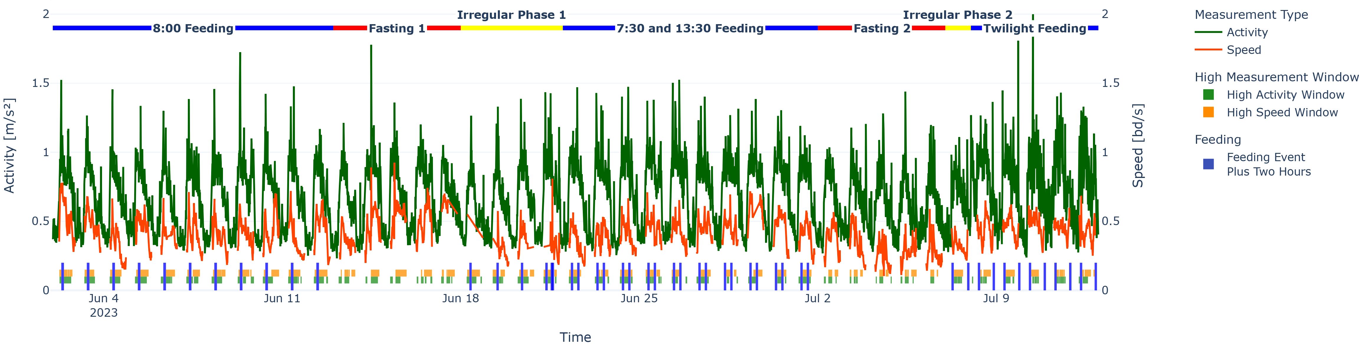
Figure 9. High-activity/speed windows plotted under the activity/speed time series for the whole experiment to show FAA and, more generally, high measurement windows. Just above the x-axis, stripes in blue indicate feeding events plus 2 h after feeding, and the two piece-wise horizontal stripes represent high measurement windows for activity (green) and speed (orange).

4 Discussion

The main findings in this study verify first and foremost the usefulness of acoustic telemetry in terms of feature detection around feeding behaviour and general animal monitoring/tracking (Li et al., 2020; Darodes de Tailly et al., 2021). Similar to our study, there are studies that concerned themselves with fish behaviour analysis through the means of using camera systems monitoring swimming speed, movements like turning speed (Miyazaki et al., 2000; Ubina et al., 2021; Priyadarshana et al., 2006; Hansen et al., 2015), or critical swimming speed (Remen et al., 2016; Yu et al., 2010), but behavioural patterns were usually qualified by humans.

Using persistent peaks as a comparison tool, we aimed to qualify the results from the camera system with the acoustic telemetry setup and conclude that movement speed could be a reliable candidate for future endeavours in fish behaviour (remote) monitoring as important features, especially around feeding, are exhibited in the speed time series.

4.1 Using persistent peaks in biological time series

Our choice to use PH for data analysis has predecessors; a wide range of fields from the medical sector [e.g., heart rate analysis (Chung et al., 2021)] over bio-molecular data analysis (Meng et al., 2020) to fish pattern analysis [e.g., quantifying zebrafish patterns (McGuirl et al., 2020)] have benefited from looking at the topological aspect of the data. In our case, using the most “significant” peaks in the time series allowed for comparison between the activity and speed time series regardless of the underlying value type (activity in m/s², speed in bd/s), since the structure of the data was the focus.

We note that an alternative method, peak detection using z-scores (Brakel, 2024; Sherathiya et al., 2021; Lima et al., 2019), though popular, was deemed inapplicable in our case for comparison of a fixed number of peaks, and would also require implicit assumptions about the peak patterns in the activity and speed time series.

4.2 Establishment of feeding patterns

We see trends of similarity in the establishment of feeding patterns for activity and speed, especially when one only considers the persistent peaks of rank 1 (see Figure 4). In both activity and speed, we see an immediate synchronisation with the feeding schedule in the “7:30 and 13:30 Feeding”. Notably, it does seem like speed retains feeding patterns much less than activity when looking at the two fasting phases, distinguishing the two locomotor activities of acceleration and speed. The wide spread of activity in the Peak 2s in Figure 4 for the phases “8:00 Feeding” and Fasting 1 could mean that fish locomotion is quite random (no pattern) as there is only one feeding time of interest. Further studies with longer feeding phases could look deeper into the concentration of secondary activities with the highest (feeding) already excluded to gain more knowledge about other fish behaviours.

Furthermore, the results of the first feeding phase in conjunction with the first fasting phase in Figure 4 align with the literature on (food-entrained) circadian rhythm in fish (Feng and Bass, 2016; Paredes et al., 2015), as we interpret the Peak 1s (activity and speed) after the feeding time as a time lag. Fasting 2 in Figure 4 indicates an inner circadian rhythm of at least more than 24 h. Furthermore, with insights from Figure 6, where the periodicity of activity is always around 24 h (never below 24 h for activity, in fact), but never reaching 25 h, we argue that the circadian rhythm of the behaviour of European seabass is potentially in that interval.

The periodicity analysis in Figure 6 illustrates that activity can potentially proxy speed data and vice versa in tracking periodic feeding patterns, since the highest deviation within the same trial was 24.00 h − 23.47 h = 0.53 h, which is around 32 min. However, we note that, because of the different translation from lags in the ACFs to minutes, the given minute difference should be taken with caution.

Moreover, the cross-correlation analysis in Section 3.2.2 shows a perfect match for activity and speed, since the highest significant values were obtained with zero lag. Nevertheless, the results for non-zero lags are also distorted due to the fact that they compare values with having 9-h time difference due to the exclusion of values outside of 6:00–21:00.

When taking a look at the depth behaviour, bright sunlight during the middle of the day was likely the main influence in the diving behaviour we observed in Figure 8. Fish avoid surface proximity during the middle of the day even around feeding time as seen before (Chen et al., 2023).

4.3 Two feedings per day

On a more general level, it does seem that the first and second feeding activity levels are synchronising after a few days as seen in Figure 8. Although in the beginning, the first feeding event was more dominant in terms of high activity values around the feeding time, the second feeding catches up towards the end of the respective feeding phases. For speed, it appears that the change is either less pronounced or not existent as the statistics in Section 3.3.2 were not significant.

On the persistent peak level, we make more detailed findings, namely, that in phase “7:30 and 13:30 Feeding”, the highest persistent peak was for both data types predominantly at the second feeding at 13:30 (see Figure 5). We postulate, together with the concentration of Peak 1s around the feeding time (see blue bars in Figure 4), that fish might be in the balancing act of avoiding the brighter upper water column, while still maximising food intake. We suggest that aligning both the feeding-entrained and the light-entrained circadian rhythm could have caused the spikes in activity and speed, respectively, as the feeding-entrained clock seems to be malleable (del Pozo et al., 2012).

For the “Twilight Feeding” phase, caution is advised, as the number of days was small (N_days = 5). While the periodicity analysis indicates that there are daily patterns (see Figure 6), they are not visible in the persistent peak analysis (see Figure 4). In contrast, the Peak 1s for activity and speed are significantly different for this feeding phase, showing an inconsistent knowledge gain from the two measurement types, activity and speed. For activity, Peak 1s are too late, and for speed, Peak 1s are too early for the closest feeding event.

Another inconsistency is also found in the mean locomotion around the feeding, as shown in Figure 8: While the speed around feeding remains stable for the “Twilight Feeding” phase regardless of the feeding event, the activity around the evening feeding is considerably lower than for the early morning feeding. It is in fact the lowest recorded activity around feeding for the whole experiment.

We conclude that maybe the European seabass in our study were not preparing for incoming evening feed. While farmed European seabass have their feeding periods during dawn and dusk in demand-feeding setups (Rubio et al., 2004), fish in our case were habituated to receive feeding during the day, which might have depressed the circadian rhythm induced by photoperiod to expect feed in the evening.

At the same time, stable speed levels around feeding speak for the notion that the circadian rhythm induced by photoperiod is not strongly linked to general movement of fish, only to (fast) acceleration. Lastly, another explanation could be that fish are not preferring meals at twilight times in general, which is also indicated by the dominant lack of FAA for both the early morning and evening (see Figure 9).

4.4 Food anticipatory behaviour analysis

The threshold for FAA duration was 60 min shorter than in Chen et al. (2023) as we included two feeding phases in this experiment and thus expected a shortening in FAA exhibition (even though it made no difference in significance whether we used 60 or 120 min for the statistics). Interestingly, activity and speed differ in the detection of FAB. Using the increases of the values in the time series, even with some parameter variations, activity could be considered a “front-runner” for FAA while higher speed values retained longer. This pattern is even consistent regardless of whether we look at feeding phases or fasting phases. A careful interpretation would be that feeding activity—and pre-feeding activity for that matter—are a type of activity that is more captured through acceleration, since the feeding action itself is more a burst towards the feed. The prolonged speed windows could potentially be explained by the assumption that speed is a more even measurement type and less “spiky”.

4.5 Comparison of activity and speed

In a sense, we used acoustic transmitters to qualify camera readings in this study and have mixed results. Firstly, there are different advantages and drawbacks to each technology.

The main advantage of using acoustic telemetry is that continuous monitoring is feasible without artificial light and that acoustics do not attenuate underwater as fast as light. This makes analysis of welfare and general fish behaviour more comprehensible, since the individual level can always be considered if desired.

The main drawback of using acoustic telemetry is that operational costs can be resource-consuming. Tags are expensive, making tagging of many individuals hardly feasible, which, in turn, can lead to questions about the representativeness of the tagged fish. Furthermore, when tagging fish, one has to ensure that the implantation does not affect the fish behaviour. As seen in Section 2.2.1, we dealt with the possible effects of implantation on behaviour by waiting at least 14 days before beginning behavioural monitoring in accordance with the results of Georgopoulou et al. (2022). Another limitation can be battery life—the main reason the last feeding phase in this study fell short (N_days = 5) in the data collection phase as transmitters stopped sending signals. Lastly, as in our study, analysis often has to be done post-experiment if the acoustic receivers cannot transmit data in real time. Note that some of the mentioned issues can be alleviated with acoustic telemetry systems that allow real-time monitoring (Hassan et al., 2019; Manicacci et al., 2022).

The main advantage of using cameras like in this experiment is that the setup can be integrated in net pen setups without many complications, making it suitable for commercial fish farming. Additionally, the gained video data can be revisited at any later stage as computer vision is advancing at a considerable speed, which may allow further post-experiment analysis. Furthermore, the agnostic nature of cameras in terms of individuality allows for an overview of the net pen status.

The main drawback of using camera systems is that they are light and sight dependent (i.e., photoperiod and turbidity) and therefore cannot provide true 24-h time series without assumptions or interpolations. Dealing with this type of time series that has gaps of the type “Missing not at random” (MNAR) (Rubin, 1976) is arguably the most challenging one, since we cannot properly correct for biases if the conducting analysis had introduced them (Mack et al., 2018). Comparing time series with gaps against true 24-h time series, errors might be induced. An additional drawback of camera analysis is the lack of depth range (Føre et al., 2018), which, with occlusion, also limits the usage for individual tracking. Some of these issues could be solved by using infrared cameras as in future works, though the trade-off would be observation range (Babin and Stramski, 2002; Hale and Querry, 1973). In addition, multiple cameras could alleviate the issue of calculating 2D trajectories in a 3D world, even though we handled this in our experiment by normalising speed according to fish size (Georgopoulou et al., 2024). Moreover, as seen in Section 3.3.2 or Section 3.3.3, changes in speed seem to lag behind or are less responsive than acoustic telemetry data, which might be explained by the fact that individual fish behaviour in sea cages does need time to propagate throughout the school of fish. Lastly, at least in our case, the speed time series is somewhat not stable in regard to the wavelet power transform. While the activity time series does deliver a spectrum reflecting the experiment protocol, the speed power spectrum does not (see Figure 7; Supplementary Figure S2).

Going over to the similarities, there are some key aspects that indicate that speed and activity can be used interchangeably: Both data types catch pattern changes throughout the experiment (see Section 3.1.2 and Section 3.1.4), though some knowledge gaps remain for the “Twilight Feeding” phase. Likewise, the actual local maxima, the persistent peaks of rank 1, tend to align during feeding, with the phase “Twilight Feeding” excluded. Similarly, the measurements around the feeding times (see Figure 8) were especially stable in the phase “7:30 and 13:30 Feeding”, but both data types in the persistent peak distribution in Figure 5 revealed high noon feeding locomotion. That this specific behaviour could be recorded with both acoustics and visual sensors indicates that a certain degree of interchangeability exists. Lastly, the periodicity analysis based on autocorrelation indicates that general patterns are caught by both data types reliably, even though the retention qualities may differ (see Figure 6).

All in all, behaviour analysis that needs fast responses from the fish or is focused on nighttime activity could benefit from using acoustic transmitters if equipped with the possibility of real-time data extraction. In order to gain an overview of group behaviour, on the other hand, one might benefit from camera setups for speed inference.

We anticipate that camera setups invite less downstream concerns, especially in commercial settings, than implanted transmitters and therefore are suitable to guide feeding optimisation and fish behaviour monitoring for remote applications. Nonetheless, using both technologies in parallel naturally yields a more holistic view on fish behaviour in sea cages and could be used in a qualifying manner when testing new fish farming protocols.

4.6 Limitations of the study

First and foremost, we make it clear that we do not claim that there is a direct cause–effect relationship between measured activity and speed, as any found correlation is likely spurious with fish locomotion work in general as a confounding factor. Because fish move at all, we can record activity from acceleration and speed from tracking individuals and averaging; therefore, both measurements come from the same source.

Secondly, using persistent peaks might introduce biases or other skewness, since we first applied the peak analysis on the raw data and then analysed these results. The intermediate layer of persistent peaks might be faulty, even though we avoided the pitfall of conducting statistical analysis or machine learning directly on persistence values themselves (Cao et al., 2024), but only on the ranking of persistent peaks.

Thirdly, by having irregular phases (see Table 1) in the experiment, the generated data for the feeding phases could be somewhat distorted. The error would then propagate through the entire analysis. Additionally, there is an absence of both biological and technical replicates; therefore, further work is needed to verify the trends and implications of the results.

Lastly, one potential limitation is that we did not reflect the whole sea cage with both sensor systems. In the worst case, fish that occluded conspecifics for the camera and the tagged fish exhibited a certain behaviour not shared by the rest of the sea cage fish, therefore giving us a false impression of the underlying mechanisms in fish behaviour.

4.7 Future work

Future work could entail controlled manipulation and testing of environmental factors such as water temperature, salinity, and light in order to make presented results more robust, as fish behaviour might differ in various environments. In order to generalise the results from this study, bigger sample sizes for acoustic telemetry would also be beneficial. Additionally, conducting similar studies on other farmed fish species and more fish sizes could improve current findings.

Another interesting study direction would be exploring the potential complete substitution of one technology for the other. However, one should take into account that both measurement types have inherently different properties, such as the spikiness of activity and retaining of high measurement windows of speed before exchanging one technology for the other.

Data availability statement

The transmitter dataset and the speed dataset for this study can be found under the DOI 10.5281/zenodo.12999133 and is licensed under the Creative Commons CC-BY 4.0 license. The latest code release of the Python code used for this study is licensed under the Apache License 2.0 and can be found under the DOI: 10.5281/zenodo.12997571. Please note that, due to similar or same type, format and structure of the acoustic transmitter dataset of this study and a previous explored one (data under DOI: 10.5281/zenodo.7900274), pieces of code from this study’s repository were heavily inspired or identical to previous published code, under the DOI 10.5281/zenodo.7977064 which belongs to the paper under DOI 10.3389/fmars.2023.1168953, or namely Chen et al. (2023).

Ethics statement

The animal study was approved by the Ethics Committee of the IMBBC and the relevant veterinary authorities (Ref Number 32257 09-02-2021), all in accordance with legal regulations (EU Directive 2010/63). The study was conducted in accordance with the local legislation and institutional requirements.

Author contributions

I-HC: Conceptualization, Data curation, Formal analysis, Methodology, Software, Visualization, Writing – original draft, Writing – review & editing. DG: Conceptualization, Data curation, Formal analysis, Methodology, Visualization, Writing – review & editing. LE: Conceptualization, Formal analysis, Funding acquisition, Investigation, Project administration, Resources, Supervision, Validation, Writing – review & editing. DV: Data curation, Investigation, Validation, Writing – review & editing. AM-K: Formal analysis, Methodology, Writing – review & editing. NP: Conceptualization, Data curation, Formal analysis, Funding acquisition, Investigation, Methodology, Project administration, Resources, Supervision, Validation, Writing – review & editing.

Funding

The author(s) declare financial support was received for the research, authorship, and/or publication of this article. This work was funded by the iFishIENCi project and has received funding from the European Union’s Horizon 2020 research and innovation program under grant agreement no. 818036 and the Norwegian Research Council, Project number 323300.

Acknowledgments

The authors thank Laura Weingott for their contribution in visualising Figure 5.

Conflict of interest

The authors declare that the research was conducted in the absence of any commercial or financial relationships that could be construed as a potential conflict of interest.

Publisher’s note

All claims expressed in this article are solely those of the authors and do not necessarily represent those of their affiliated organizations, or those of the publisher, the editors and the reviewers. Any product that may be evaluated in this article, or claim that may be made by its manufacturer, is not guaranteed or endorsed by the publisher.

Supplementary material

The Supplementary Material for this article can be found online at: https://www.frontiersin.org/articles/10.3389/fmars.2024.1497336/full#supplementary-material

References

Alfonso S., Zupa W., Spedicato M. T., Lembo G., Carbonara P. (2022). Using telemetry sensors mapping the energetic costs in european sea bass (Dicentrarchus labrax), as a tool for welfare remote monitoring in aquaculture. Front. Anim. Sci. 3. doi: 10.3389/fanim.2022.885850

Crossref Full Text | Google Scholar

Al-Jubouri Q., Al-Nuaimy W., Al-Taee M. A., Young I. (2017). “Computer stereovision system for 3D tracking of free-swimming zebrafish (Institute of Electrical and Electronics Engineers Inc.),” in 2017 10th International Conference on Developments in eSystems Engineering (DeSE), Paris, France. pp. 188–192. doi: 10.1109/DeSE.2017.31

Crossref Full Text | Google Scholar

AlZubi H. S., Al-Nuaimy W., Buckley J., Young I. (2016). “An intelligent behavior-based fish feeding system,” in 2016 13th International Multi-Conference on Systems, Signals & Devices (SSD), Leipzig, Germany. 22–29 (IEEE). doi: 10.1109/SSD.2016.7473754

Crossref Full Text | Google Scholar

An D., Hao J., Wei Y., Wang Y., Yu X. (2021). Application of computer vision in fish intelligent feeding system—A review. Aquaculture Res. 52, 423–437. doi: 10.1111/are.14907

Crossref Full Text | Google Scholar

Azzaydi M., Rubio V. C., Lopez F. J. M., Sánchez-Vázquez F. J., Zamora S., Madrid J. A. (2007). Effect of restricted feeding schedule on seasonal shifting of daily demand-feeding pattern and food anticipatory activity in European sea bass (Dicentrarchus labrax L.). Chronobiol. Int. 24, 859–874. doi: 10.1080/07420520701658399

PubMed Abstract | Crossref Full Text | Google Scholar

Babin M., Stramski D. (2002). Light absorption by aquatic particles in the near-infrared spectral region. Limnol. Oceanogr. 47, 911–915. doi: 10.4319/lo.2002.47.3.0911

PubMed Abstract | Crossref Full Text | Google Scholar

Brakel J. v. (2024). Robust peak detection algorithm (using z-scores). Available online at: https://stackoverflow.com/questions/22583391/peak-signal-detection-in-realtime-timeseriesdata/2264036222640362 (Accessed April 17th, 2024).

Google Scholar

Cao Y., Leung P., Monod A. (2024). k-means clustering for persistent homology. Adv. Data Anal. Classification. doi: 10.1007/s11634-023-00578-y

Crossref Full Text | Google Scholar

Carbonara P., Alfonso S., Dioguardi M., Zupa W., Vazzana M., Dara M., et al. (2021). Calibrating accelerometer data, as a promising tool for health and welfare monitoring in aquaculture: Case study in European sea bass (Dicentrarchus labrax) in conventional or organic aquaculture. Aquaculture Rep. 21, 100817. doi: 10.1016/j.aqrep.2021.100817

Crossref Full Text | Google Scholar

Chazal F., Michel B. (2021). An introduction to topological data analysis: fundamental and practical aspects for data scientists. Front. Artif. Intell. 4. doi: 10.3389/frai.2021.667963

PubMed Abstract | Crossref Full Text | Google Scholar

Chen I.-H., Georgopoulou D. G., Ebbesson L. O. E., Voskakis D., Lal P., Papandroulakis N. (2023). Food anticipatory behaviour on European seabass in sea cages: activity-, positioning-, and density-based approaches. Front. Mar. Sci. 10. doi: 10.3389/fmars.2023.1168953

Crossref Full Text | Google Scholar

Chuang M. C., Hwang J. N., Williams K., Towler R. (2015). Tracking live fish from low-contrast and low-frame-rate stereo videos. IEEE Trans. Circuits Syst. Video Technol. 25, 167–179. doi: 10.1109/TCSVT.2014.2357093

Crossref Full Text | Google Scholar

Chung Y.-M., Hu C.-S., Lo Y.-L., Wu H.-T. (2021). A persistent homology approach to heart rate variability analysis with an application to sleep-wake classification. Front. Physiol. 12. doi: 10.3389/fphys.2021.637684

PubMed Abstract | Crossref Full Text | Google Scholar

Cohen-Steiner D., Edelsbrunner H., Harer J. (2007). enStability of persistence diagrams. Discrete Comput. Geometry 37, 103–120. doi: 10.1007/s00454-006-1276-5

Crossref Full Text | Google Scholar

Darodes de Tailly J.-B., Keitel J., Owen M. A., Alcaraz-Calero J. M., Alexander M. E., Sloman K. A. (2021). enMonitoring methods of feeding behaviour to answer key questions in penaeid shrimp feeding. Rev. Aquaculture 13, 1828–1843. doi: 10.1111/raq.12546

Crossref Full Text | Google Scholar

del Pozo A., Montoya A., Vera L. M., Sánchez-Vázquez F. J. (2012). Daily rhythms of clock gene expression, glycaemia and digestive physiology in diurnal/nocturnal European seabass. Physiol. Behav. 106, 446–450. doi: 10.1016/j.physbeh.2012.03.006

PubMed Abstract | Crossref Full Text | Google Scholar

Edelsbrunner H., Harer J. (2008). Persistent homology—a survey. Discrete Comput. Geometry - DCG 453, 257–282. doi: 10.1090/conm/453/08802

Crossref Full Text | Google Scholar

Edelsbrunner, Letscher, Zomorodian (2002). Topological persistence and simplification. Discrete Comput. Geometry 28, 511–533. doi: 10.1007/s00454-002-2885-2

Crossref Full Text | Google Scholar

FAO (2024). The State of World Fisheries and Aquaculture 2024 – Blue Transformation in action (Rome: FAO).

Google Scholar

Feng N. Y., Bass A. H. (2016). Singing” Fish rely on circadian rhythm and melatonin for the timing of nocturnal courtship vocalization. Curr. Biol. 26, 2681–2689. doi: 10.1016/j.cub.2016.07.079

PubMed Abstract | Crossref Full Text | Google Scholar

Føre M., Svendsen E., Alfredsen J. A., Uglem I., Bloecher N., Sveier H., et al. (2018). Using acoustic telemetry to monitor the effects of crowding and delousing procedures on farmed Atlantic salmon (Salmo salar). Aquaculture 495, 757–765. doi: 10.1016/j.aquaculture.2018.06.060

Crossref Full Text | Google Scholar

Foster M., Petrell R., Ito M. R., Ward R. (1995). Detection and counting of uneaten food pellets in a sea cage using image analysis. Aquacultural Eng. 14, 251–269. doi: 10.1016/0144-8609(94)00006-M

Crossref Full Text | Google Scholar

Fugacci U., Scaramuccia S., Iuricich F., Floriani L. D. (2016). Persistent homology: a step-by-step introduction for newcomers. 1–10. doi: 10.2312/stag.20161358

Crossref Full Text | Google Scholar

Georgopoulou D. G., Fanouraki E., Voskakis D., Mitrizakis N., Papandroulakis N. (2022). European seabass show variable responses in their group swimming features after tag implantation. Front. Anim. Sci. 3, 997948. doi: 10.3389/fanim.2022.997948

Crossref Full Text | Google Scholar

Georgopoulou D. G., Vouidaskis C., Papandroulakis N. (2024). Swimming behavior as a potential metric to detect satiation levels of European seabass in marine cages. Front. Mar. Sci. 11. doi: 10.3389/fmars.2024.1350385

Crossref Full Text | Google Scholar

Hale G. M., Querry M. R. (1973). Optical constants of water in the 200-nm to 200-m wavelength region. Appl. Optics 12, 555–563. doi: 10.1364/AO.12.000555

PubMed Abstract | Crossref Full Text | Google Scholar

Han F., Zhu J., Liu B., Zhang B., Xie F. (2020). Fish shoals behavior detection based on convolutional neural network and spatiotemporal information. IEEE Access 8, 126907–126926. doi: 10.1109/ACCESS.2020.3008698

Crossref Full Text | Google Scholar

Hansen M. J., Schaerf T. M., Ward A. J. W. (2015). enThe influence of nutritional state on individual and group movement behaviour in shoals of crimson-spotted rainbowfish (Melanotaenia duboulayi). Behav. Ecol. Sociobiol. 69, 1713–1722. doi: 10.1007/s00265-015-1983-0

Crossref Full Text | Google Scholar

Hassan W., Føre M., Ulvund J. B., Alfredsen J. A. (2019). Internet of Fish: Integration of acoustic telemetry with LPWAN for efficient real-time monitoring of fish in marine farms. Comput. Electron. Agric. 163, 104850. doi: 10.1016/j.compag.2019.06.005

Crossref Full Text | Google Scholar

Hu W. C., Chen L. B., Huang B. K., Lin H. M. (2022). A computer vision-based intelligent fish feeding system using deep learning techniques for aquaculture. IEEE Sensors J. 22, 7185–7194. doi: 10.1109/JSEN.2022.3151777

Crossref Full Text | Google Scholar

Hu X., Liu Y., Zhao Z., Liu J., Yang X., Sun C., et al. (2021). Real-time detection of uneaten feed pellets in underwater images for aquaculture using an improved YOLO-V4 network. Comput. Electron. Agric. 185, 106135. doi: 10.1016/j.compag.2021.106135

Crossref Full Text | Google Scholar

Huber S. (2017). Persistent topology for peak detection. Available online at: https://www.sthu.org/blog/13perstopology-peakdetection/index.html (Accessed June 6th, 2024).

Google Scholar

Huber S. (2021). “dePersistent Homology in Data Science,” in Data Science – Analytics and Applications. Eds. Haber P., Lampoltshammer T., Mayr M., Plankensteiner K. (Springer Fachmedien, Wiesbaden), 81–88. doi: 10.1007/978-3-658-32182-613

Crossref Full Text | Google Scholar

Jacoby D. M. P., Piper A. T. (2023). What acoustic telemetry can and cannot tell us about fish biology. J. Fish Biol.. 1–25. doi: 10.1111/jfb.15588

PubMed Abstract | Crossref Full Text | Google Scholar

Jepsen N., Schreck C., Clements S., Thorstad E. (2005). “A brief discussion on the 2% tag/bodymass rule of thumb,” in 5th Conference on Fish Telemetry - Ustica, Italy. Aquatic telemetry: advances and applications. 255–259 (Food and Agriculture Organization of the United Nations).

Google Scholar

Kolarevic J., Aas-Hansen E., Baeverfjord G., Terjesen B. F., Damsgard B. (2016). The use of acoustic acceleration transmitter tags for monitoring of Atlantic salmon swimming activity in recirculating aquaculture systems (RAS). Aquacultural Eng. 72-73, 30–39. doi: 10.1016/j

PubMed Abstract | Crossref Full Text | Google Scholar

Kong Q., Du R., Duan Q., Zhang Y., Chen Y., Li D., et al. (2022). A recurrent network based on active learning for the assessment of fish feeding status. Comput. Electron. Agric. 198, 106979. doi: 10.1016/j.compag.2022.106979

Crossref Full Text | Google Scholar

Lédée E. J. I., Heupel M. R., Taylor M. D., Harcourt R. G., Jaine F. R. A., Huveneers C., et al. (2021). Continental-scale acoustic telemetry and network analysis reveal new insights into stock structure. Fish Fisheries 22, 987–1005. doi: 10.1111/faf.12565

Crossref Full Text | Google Scholar

Leroy B., Scutt Phillips J., Potts J., Brill R. W., Evans K., Forget F., et al. (2023). Recommendations towards the establishment of best practice standards for handling and intracoelomic implantation of data-storage and telemetry tags in tropical tunas. Anim. Biotelemetry 11, 4. doi: 10.1186/s40317-023-00316-3

Crossref Full Text | Google Scholar

Li D., Du Z., Wang Q., Wang J., Du L. (2024a). Recent advances in acoustic technology for aquaculture: A review. Rev. Aquaculture 16, 357–381. doi: 10.1111/raq.12842

Crossref Full Text | Google Scholar

Li D., Wang Z., Wu S., Miao Z., Du L., Duan Y. (2020). Automatic recognition methods of fish feeding behavior in aquaculture: A review. Aquaculture (Amsterdam Netherlands) 528, 735508. doi: 10.1016/j.aquaculture.2020.735508

Crossref Full Text | Google Scholar

Li D., Yu J., Du Z., Xu W., Wang G., Zhao S., et al. (2024b). Advances in the application of stereo vision in aquaculture with emphasis on fish: A review. Rev. Aquaculture 16, 1718–1740. doi: 10.1111/raq.12919

Crossref Full Text | Google Scholar

Lima B. M. R., Ramos L. C. S., de Oliveira T. E. A., da Fonseca V. P., Petriu E. M. (2019). Heart rate detection using a multimodal tactile sensor and a Z-score based peak detection algorithm. CMBES Proc. 42. Retrieved from https://proceedings.cmbes.ca/index.php/proceedings/article/view/850.

Google Scholar

Liu Z., Li X., Fan L., Lu H., Liu L., Liu Y. (2014). Measuring feeding activity of fish in RAS using computer vision. Aquacultural Eng. 60, 20–27. doi: 10.1016/j.aquaeng.2014.03.005

Crossref Full Text | Google Scholar

López-Olmeda J. F., Noble C., Sánchez-Vázquez F. J. (2012). enDoes feeding time affect fish welfare? Fish Physiol. Biochem. 38, 143–152. doi: 10.1007/s10695-011-9523-y

PubMed Abstract | Crossref Full Text | Google Scholar

Macaulay G., Bui S., Oppedal F., Dempster T. (2021a). Challenges and benefits of applying fish behaviour to improve production and welfare in industrial aquaculture. Rev. Aquaculture 13, 934–948. doi: 10.1111/raq.12505

Crossref Full Text | Google Scholar

Macaulay G., Warren-Myers F., Barrett L. T., Oppedal F., Føre M., Dempster T. (2021b). Tag use to monitor fish behaviour in aquaculture: a review of benefits, problems and solutions. Rev. Aquaculture 13, 1565–1582. doi: 10.1111/raq.12534

Crossref Full Text | Google Scholar

Mack C., Su Z., Westreich D. (2018). “Types of Missing Data,” in Managing Missing Data in Patient Registries: Addendum to Registries for Evaluating Patient Outcomes: A User’s Guide, 3rd ed. (Agency for Healthcare Research and Quality, US).

Google Scholar

Malott N. O., Chen S., Wilsey P. A. (2023). A survey on the high-performance computation of persistent homology. IEEE Trans. Knowledge Data Eng. 35, 4466–4484. doi: 10.1109/TKDE.2022.3147070

Crossref Full Text | Google Scholar

Måløy H., Aamodt A., Misimi E. (2019). A spatio-temporal recurrent network for salmon feeding action recognition from underwater videos in aquaculture. Comput. Electron. Agric. 167, 105087. doi: 10.1016/j.compag.2019.105087

Crossref Full Text | Google Scholar

Manicacci F.-M., Mourier J., Babatounde C., Garcia J., Broutta M., Gualtieri J.-S., et al. (2022). enA wireless autonomous real-time underwater acoustic positioning system. Sensors 22, 8208. doi: 10.3390/s22218208

PubMed Abstract | Crossref Full Text | Google Scholar

Martins C. I. M., Galhardo L., Noble C., Damsgård B., Spedicato M. T., Zupa W., et al. (2012). Behavioural indicators of welfare in farmed fish. Fish Physiol. Biochem. 38, 17–41. doi: 10.1007/s10695-011-9518-8

PubMed Abstract | Crossref Full Text | Google Scholar

McGuirl M. R., Volkening A., Sandstede B. (2020). Topological data analysis of zebrafish patterns. Proc. Natl. Acad. Sci. 117, 5113–5124. doi: 10.1073/pnas.1917763117

PubMed Abstract | Crossref Full Text | Google Scholar

Meng Z., Anand D. V., Lu Y., Wu J., Xia K. (2020). Weighted persistent homology for biomolecular data analysis. Sci. Rep. 10, 2079. doi: 10.1038/s41598-019-55660-3

PubMed Abstract | Crossref Full Text | Google Scholar

Miyazaki T., Masuda R., Furuta S., Tsukamoto K. (2000). Feeding behaviour of hatcheryreared juveniles of the Japanese flounder following a period of starvation. Aquaculture 190, 129–138. doi: 10.1016/S0044-8486(00)00385-9

Crossref Full Text | Google Scholar

Munch E. (2017). A user’s guide to topological data analysis. J. Learn. Analytics 4, 47–61. doi: 10.18608/jla.2017.42.6

Crossref Full Text | Google Scholar

Neo Y. Y., Hubert J., Bolle L. J., Winter H. V., Slabbekoorn H. (2018). European seabass respond more strongly to noise exposure at night and habituate over repeated trials of sound exposure. Environ. pollut. 239, 367–374. doi: 10.1016/j.envpol.2018.04.018

PubMed Abstract | Crossref Full Text | Google Scholar

Niu B., Li G., Peng F., Wu J., Zhang L., Li Z. (2018). Survey of fish behavior analysis by computer vision. J. Aquaculture Res. Dev. 9, 534. doi: 10.4172/2155-9546.1000534

Crossref Full Text | Google Scholar

Orduna C., Encina L., Rodr´ıguez-Ruiz A., Rodríguez-Sánchez V. (2021). Hydroacoustics for density and biomass estimations in aquaculture ponds. Aquaculture 545, 737240. doi: 10.1016/j.aquaculture

Crossref Full Text | Google Scholar

Paredes J. F., López-Olmeda J. F., Mart´ınez F. J., Sánchez-Vázquez F. J. (2015). Daily rhythms of lipid metabolic gene expression in zebra fish liver: Response to light/dark and feeding cycles. Chronobiol. Int. 32, 1438–1448. doi: 10.3109/07420528.2015.1104327

PubMed Abstract | Crossref Full Text | Google Scholar

Pautsina A., Císař P., Štys D., Terjesen B. F., Espmark M. O. (2015). Infrared reflection system for indoor 3D tracking of fish. Aquacultural Eng. 69, 7–17. doi: 10.1016/j.aquaeng.2015.09.002

Crossref Full Text | Google Scholar

Pradana H., Horio K. (2022). Automatic controlling fish feeding machine using feature extraction of nutriment and ripple behavior. doi: 10.24507/ijicic.17.05.1483

Crossref Full Text | Google Scholar

Priyadarshana T., Asaeda T., Manatunge J. (2006). enHunger-induced foraging behavior of two cyprinid fish: Pseudorasbora parva and Rasbora daniconius. Hydrobiologia 568, 341–352. doi: 10.1007/s10750-006-0201-5

Crossref Full Text | Google Scholar

Remen M., Solstorm F., Bui S., Klebert P., Vågseth T., Solstorm D., et al. (2016). enCritical swimming speed in groups of Atlantic salmon Salmo salar. Aquaculture Environ. Interact. 8, 659–664. doi: 10.3354/aei00207

Crossref Full Text | Google Scholar

Rubin D. B. (1976). Inference and missing data. Biometrika 63, 581–592. doi: 10.2307/2335739

Crossref Full Text | Google Scholar

Rubio V. C., Vivas M., Sánchez-Mut A., Sánchez-Vázquez F. J., Covès D., Dutto G., et al. (2004). Self-feeding of European sea bass (Dicentrarchus labrax, L.) under laboratory and farming conditions using a string sensor. Aquaculture 233, 393–403. doi: 10.1016/j.aquaculture.2003.10.011

Crossref Full Text | Google Scholar

Saberioon M., Gholizadeh A., Cisar P., Pautsina A., Urban J. (2017). Application of machine vision systems in aquaculture with emphasis on fish: state-of-the-art and key issues. Rev. Aquaculture 9, 369–387. doi: 10.1111/raq.12143

Crossref Full Text | Google Scholar

Samedy V., Wach M., Lobry J., Selleslagh J., Pierre M., Josse E., et al. (2015). Hydroacoustics as a relevant tool to monitor fish dynamics in large estuaries. Fisheries Res. 172, 225–233. doi: 10.1016/j.fishres.2015.07.025

Crossref Full Text | Google Scholar

Samori E. (2024). Daily rhythms of physiological processes in fish: synchronization to light and feeding cycles and effects on the molecular clock, epigenetics and welfare (Universidad de Murcia). Available online at: http://purl.org/dc/dcmitype/Text (Accessed December 15th, 2024).

Google Scholar

Sherathiya V. N., Schaid M. D., Seiler J. L., Lopez G. C., Lerner T. N. (2021). GuPPy, a Python toolbox for the analysis of fiber photometry data. Sci. Rep. 11, 24212. doi: 10.1038/s41598-021-03626-9

PubMed Abstract | Crossref Full Text | Google Scholar

Stockwell C. L., Filgueira R., Grant J. (2021). Determining the effects of environmental events on cultured Atlantic salmon behaviour using 3-dimensional acoustic telemetry. Front. Anim. Sci. 2. doi: 10.3389/fanim.2021.701813

Crossref Full Text | Google Scholar

Torisawa S., Kadota M., Komeyama K., Suzuki K., Takagi T. (2011). A digital stereo-video camera system for three-dimensional monitoring of free-swimming Pacific bluefin tuna, Thunnus orientalis, cultured in a net cage. Aquat. Living Resour. 24, 107–112. doi: 10.1051/alr/2011133

Crossref Full Text | Google Scholar

Ubina N., Cheng S.-C., Chang C.-C., Chen H.-Y. (2021). Evaluating fish feeding intensity in aquaculture with convolutional neural networks. Aquacultural Eng. 94, 102178. doi: 10.1016/j.aquaeng.2021.102178

Crossref Full Text | Google Scholar

Verdegem M., Buschmann A. H., Latt U. W., Dalsgaard A. J. T., Lovatelli A. (2023). enThe contribution of aquaculture systems to global aquaculture production. J. World Aquaculture Soc. 54, 206–250. doi: 10.1111/jwas.12963

Crossref Full Text | Google Scholar

Wagner G. N., Cooke S. J., Brown R. S., Deters K. A. (2011). Surgical implantation techniques for electronic tags in fish. Rev. Fish Biol. Fisheries 21, 71–81. doi: 10.1007/s11160-010-9191-5

Crossref Full Text | Google Scholar

Wang Q., Long W., Wang Y., Jiang L., Hu L. (2021). “Fish behavior detection using computer vision: a review,” in 2021 3rd International Conference on Artificial Intelligence and Advanced Manufacture (AIAM), Manchester, United Kingdom. pp. 375–381. doi: 10.1109/AIAM54119.2021.00082

Crossref Full Text | Google Scholar

Wang Y., Yu X., Liu J., An D., Wei Y. (2022). Dynamic feeding method for aquaculture fish using multi-task neural network. Aquaculture 551, 737913. doi: 10.1016/j.aquaculture.2022.737913

Crossref Full Text | Google Scholar

Yang L., Liu Y., Yu H., Fang X., Song L., Li D., et al. (2021a). Computer vision models in intelligent aquaculture with emphasis on fish detection and behavior analysis: A review. Arch. Comput. Methods Eng. 28, 2785–2816. doi: 10.1007/s11831-020-09486-2

Crossref Full Text | Google Scholar

Yang X., Zhang S., Liu J., Gao Q., Dong S., Zhou C. (2021b). Deep learning for smart fish farming: applications, opportunities and challenges. Rev. Aquaculture 13, 66–90. doi: 10.1111/raq.12464

Crossref Full Text | Google Scholar

Yu X., Zhang X., Duan Y., Zhang P., Miao Z. (2010). Effects of temperature, salinity, body length, and starvation on the critical swimming speed of whiteleg shrimp, Litopenaeus vannamei. Comp. Biochem. Physiol. Part A: Mol. Integr. Physiol. 157, 392–397. doi: 10.1016/j.cbpa.2010.08.021

PubMed Abstract | Crossref Full Text | Google Scholar

Zhou C., Lin K., Xu D., Chen L., Guo Q., Sun C., et al. (2018a). Near infrared computer vision and neuro-fuzzy model-based feeding decision system for fish in aquaculture. Comput. Electron. Agric. 146, 114–124. doi: 10.1016/j.compag.2018.02.006

Crossref Full Text | Google Scholar

Zhou C., Xu D., Lin K., Sun C., Yang X. (2018b). Intelligent feeding control methods in aquaculture with an emphasis on fish: a review. Rev. Aquaculture 10, 975–993. doi: 10.1111/raq.12218

Crossref Full Text | Google Scholar

Zhou C., Zhang B., Lin K., Xu D., Chen C., Yang X., et al. (2017). Near-infrared imaging to quantify the feeding behavior of fish in aquaculture. Comput. Electron. Agric. 135, 233–241. doi: 10.1016/j.compag.2017.02.013

Crossref Full Text | Google Scholar