Real-time ocean wave prediction in time domain with autoregression and echo state networks

This study evaluates the potential of applying echo state networks (ESN) and autoregression (AR) for dynamic time series prediction of free surface elevation for use in wave energy converters (WECs). The performance of these models is evaluated on time series data at different water depths and wave conditions, including both measured and simulated data with a focus on real-time prediction of ocean waves at a given location without resolving for the surrounding ocean surface, in other words, short-time single-point forecasting. The work presented includes training the models on historical wave data and testing their ability to predict phase-resolved future surface wave patterns for short-time forecasts. Additionally, this study discusses the feasibility of deploying these models for extended time intervals. It provides valuable insights into the trade-offs between accuracy and practicality in the real-time implementation of predictive models for wave elevation, which are needed in wave energy converters to optimise the control algorithm.

1 Introduction

Renewable energy resources are increasingly contributing to the world’s energy generation, and ocean waves have emerged as a significant competitor to offshore wind power. Indeed, ocean power is a promising renewable energy source with an estimated resource potential of 2 TW based on average wave energy density and global coastline length (Cruz, 2008). Since the first wave farm in Portugal started operation in 2008, the substantial potential of wave energy has led to the establishment of wave power farms in various countries, aiming to harness energy from the ocean (Ringwood et al., 2014; Ge and Kerrigan, 2016). In most wave energy converters, the energy conversion is based on the relative oscillation between bodies or oscillating pressure distributions within fixed or moving chambers. As explained in Budar and Falnes (1975), in order to exploit inherent resonances in these systems, the energy converter needs to be controlled in an appropriate way. In fact, it can be shown that a well-designed control algorithm can significantly enhance the power take-up of the WEC (Falnes, 2007; Ringwood et al., 2014; Falnes and Kurniawan, 2020) and also reduce stress on the components (Laporte Weywada et al. (2021)). Real-time control of wave energy converters in turn, requires accurate forecasting of future incident wave elevation, and this is the main topic of the present contribution.

In Fusco (2009) and Fusco and Ringwood (2010), an AR model for short-time wave forecasting and real-time control for WECs was introduced and initiated in some cases from low-pass filtered wave data. To improve the accuracy of short-time prediction models, the high-frequency components in the wave records are removed by realising a low-pass filter. Different approaches are suggested for enhancing the traditional AR model for multi-step ahead prediction for system control of WECs. Fusco (2009) proposed updating the AR parameters when new data are received using recursive least squares (RLS) with a forgetting parameter. There are some trade-offs with this method such as the low-pass filter introduces a delay that needs to be compensated for by adjusting the original wave record, there is no method to determine the forgetting parameter, and after a specific time, the magnitude of the AR coefficients calculated by RLS may explode (Fusco, 2009; Ge and Kerrigan, 2016).Another approach was to minimise the error of a set of multi-step ahead prediction equations to find the AR coefficients that best describe the surface elevation instead of solving a linear ordinary least square problem (OLS) (Fusco and Ringwood, 2010). Other methods examined by Fusco and Ringwood (2010) are neural network, cyclical model and sinusoidal extrapolation with the extended Kalman filter, but all of these were found to be less promising methods for WECs than AR.

The wave records used in Fusco and Ringwood (2010) were from buoys moored in 20 and 40 meters depth. The wavelength-to-depth ratio is too small to classify as shallow water, and based on the data used, it appears that a model with an inherently linear bias such as the AR model is sufficient, and there is no need for using methods allowing nonlinear effects, and this is also borne out in the results in Fusco and Ringwood (2010). Now wave energy devices can be placed at more or less any depth (Drew et al., 2009), and wave forecasting in shallow water may require methods which are more adept at handling highly nonlinear signals expected due to the shoaling waves (see Cervantes et al. (2021) and references therein). In the present paper, we set out to test a certain type of artificial neural network, the so-called Echo State Network (ESN) which was introduced in Jaeger and Haas (2004). Considering the ESN architecture with a large reservoir of non-linearly interconnected neurons and a single dedicated output neuron, this type of network appears to be perfectly suited for predicting ocean waves, particularly for large waveheights where non-linearity is expected to be a dominant factor. In addition, since only one layer of weights (connecting to the output neuron) needs to be tuned, updating the network weights can be done efficiently and quickly.

The main aim of the present work is to investigate the actual performance of a short-term wave prediction model under realistic conditions, and we take an approach which we believe is necessary to successfully run a wave signal prediction in real-time for several hours. Consequently, the present work’s short-time ocean wave prediction is based on the original wave record rather than the corresponding low-pass filtered record. This approach also ensures a fair comparison between the AR and ESN approaches. As will come to light, both AR and ESN are viable approaches for optimising WEC in water depths of about 5 to 30 meters. Both models accurately predict the wave phase over 4 hours with a 20-second prediction horizon without calibrating the models. The advantage of the AR models calculated with ordinary least squares is that they can work effectively with limited access to data and are computationally cheap. ESN models require more data for training but can make predictions over a longer time horizon without recalculating the network’s output weights.

2 Available time series data

We utilise various types of surface ocean data to compare the performance of the different short-time prediction models and evaluate their potential for real-time implementation in WECs. This includes shallow, intermediate, and deep-water data, encompassing real-world measurements and simulated data. These diverse datasets offer a comprehensive basis for assessing and validating the wave prediction models in this study.

The simulated data are generated using the JONSWAP spectrum for deep-water time series simulation and the Bossinesq Surf and Ocean Model (BOSZ) for various water depths Roeber et al. (2010); Matysiak et al. (2024). JONSWAP simulations provide a time series with a sample rate of 1.25 Hz at infinite water depth and a frequency spectrum between 0.04 Hz and 1.25 Hz. For the JONSWAP data, the significant wave height is 1.9 meters, and the significant wave period is 11.2 seconds.

Conversely, Boussinesq models such as BOSZ allow us to study nonlinear nearshore wave processes at depths of 30 meters or less. The data used here have a sampling rate of 1 Hz and a time series length of 2 hours. The spectrum of the simulation is divided into central frequency bins between 0.03 Hz and 0.16 Hz (Matysiak et al., 2024). In this study, we used data generated by BOSZ with a number of sea states. The significant wave height H_s varies between 0.5 meters and 3.7 meters, and the significant wave period T_s varies between 7.7 and 11.1 seconds for BOSZ at 30 meters depth. For the BOSZ model output at 5 meters depth, the significant wave height varies between 0.5 and 2.2 meters, and the significant wave period varies between 7.6 and 16.6 seconds.

Buoy data is provided by the National Network of Regional Coastal Monitoring Programmes (NNRCMP) and measured at Bideford Bay in England; the wave buoy location is 51° 03.48’ N 004° 16.62’ W. The Datawell Directional WaveRider Mk III buoy was deployed on 17 June 2009 and measures surface elevation with a sampling rate of 1.28 Hz at a water depth of about 11 meters. The datasets used in the analysis are taken from 25 January to 29 January 2024 between 10:00:00 and 18:00:00 GMT (NNRCMP, 2024). The sea state in the different datasets varies, with a significant wave height between 0.8 and 1.9 meters and a significant wave period between 8.6 and 12.4 seconds.

3 Forecasting models

Most works focus on short-time prediction models that predict only seconds to hours of forecast with higher accuracy and confidence (Yevnin et al., 2023), see e.g. Duan et al. (2020); Ma et al. (2021) and Kagemoto (2020). On the other hand, long-time prediction focus on prediction of long-term statistical ocean wave properties (significant wave height, etc.) over several hours and days (Meng et al., 2022; Yevnin et al., 2023). Our study involves training and testing the models on historical wave data to predict future surface wave patterns in the seens of short-time dynamic wave prediction. This section describes the short-time prediction methods examined in the present contribution.

3.1 Autoregressive model

Assume that time series data of surface water waves can be described by a stationary stochastic linear model, a so-called autoregressive (AR) model. Here, stationary refers to second-order stationary, which means that the time series’ statistical properties, mean and variance, are time-independent and finite (Box et al., 2008).

The sea surface elevation at the current time t is denoted as $\eta (t)$ and is supposed to be linearly dependent on a number p of its past values, $\eta (t-i)$ for $t=1,2,···,p$ and a stochastic term, $є(t)$, which is supposed to be Gaussian and white noise. Equation 1 expresses mathematically an AR model of order p, where p represents the number of lagged values to include in the model (Box et al., 2008; Fusco and Ringwood, 2010).

$\begin{array}{ll}\eta (t)=\sum _{i=1}^p{a}_i\eta (t-i)+є(t)& (1)\end{array}$

The regression parameters of the autoregressive model, $a_1,a_2,···,a_p$, have the property $\left|a_i\right|<1$ for $i=1,2,···,p$ to represent a stationary process (Box et al., 2008).

When using AR as a model for predicting future surface elevation, the parameters $a_i$ are estimated as ${\widehat{a}}_i$, and the l step ahead prediction of the surface elevation at an instant time t is given by $\widehat{\eta }(t+l)$ in Equation 2.

$\begin{array}{ll}\widehat{\eta }(t+l)=\sum _{i=1}^p{\widehat{a}}_i\widehat{\eta }(t+l-i)& (2)\end{array}$

As long as $t+l-i\le t,\widehat{\eta }(t)=\eta (t)$ since the information is already acquired in the data set and there is no need for prediction (Fusco and Ringwood, 2010).

When applying machine learning techniques such as autoregression (and neural networks), hyperparameters must be determined before training the model. For example, in an autoregressive (AR) model, the order p is a key hyperparameter that must be known before estimating the coefficients ${\widehat{a}}_1,{\widehat{a}}_2,···,{\widehat{a}}_p$. These hyperparameters can be determined by splitting the data into training and testing sets, and evaluating the model’s performance on these sets.

There are different approaches for estimating the model coefficients, e.g., maximum likelihood, method of moments, and ordinary least square estimation (OLS) (Fusco and Ringwood, 2010). The coefficients can be calculated from a number n of batch wave elevation observations, $\eta (t-i)$ for all $i=1,2,···,n$, which could be written as a system of one-step ahead prediction equations, Equation 2 where $l=1$.

The AR model will be used for a multi-step ahead prediction in this contribution. So instead of minimising the OLS problem for a one-step ahead prediction, we follow the recommendations in the literature to introduce a multi-step ahead prediction cost function which is given in Equation 3. Minimising this l-step ahead cost function allows the estimation of parameters to improve the accuracy of the multi-step ahead predictions.

$\begin{array}{ll}J=\sum _{t=1}^n\sum _{j=1}^N{[\eta (t+l-j)-\widehat{\eta }(t+l-j)]}^2& (3)\end{array}$

The multi-step ahead prediction cost function J in Equation 3 quantify the error in predicting future values $\eta (t)$, using an AR model. The cost function is formulated as the sum of squared prediction errors over the prediction horizons N, and for multiple time steps n. The predicted value is denoted $\widehat{\eta }(t-j)$ with the corresponding observations, $\eta (t-j)$.The optimisation goal is to minimise the cost function given in Equation 3. This can be done using standard algorithms for solving nonlinear least square problems, such as the Gauss-Newton iteration, initialised with the OLS solution for a one-step ahead prediction (Liu et al., 1999; Fusco and Ringwood, 2010).

3.2 Echo state networks

Neural networks are machine learning models inspired by the architecture of biological brains. The standard method for training these networks is error backpropagation, a significant achievement in cognitive processes. Echo state networks (ESNs) are an alternative to backpropagation based RNNs. ESN is a simple type of RNN, mainly known for their more efficient learning of series and signal forecasting compare to standard RNN. A key feature of ESNs is their nonlinear behaviour, and in order to achieve high performance with ESNs, tuning the network’s hyperparameters properly is an important step (Lukoševičius, 2012). Echo state networks are a type of RNN composed of three layers: an input layer, one single hidden layer (also known as the reservoir, and an output layer. The weights between the input layer and reservoir W_in and within the reservoir units W^r are initialised randomly and remain fixed during training. This reduces the number of parameters to train compared to traditional RNNs, where all weights are trained. Only the output weights W_out are adjusted to match task-specific data, learning to reproduce temporal patterns efficiently (Jaeger, 2001; Lukoševičius, 2012).

ESNs are applied for supervised machine learning tasks where the input signal $\mathit{u}(n)\in {ℝ}^{N_u}$ is used for training the target signal, ${\mathit{y}}^{target}\in {ℝ}^{N_y}$. Here, n represents a discrete time series, and T is the number of samples in the training dataset. The objective is to train the model output, $\mathit{y}(n)$, to match the actual measurements closely ${\mathit{y}}^{target}(n)$ by minimising the error measure $E(\mathit{y}(n),{\mathit{y}}^{target}(n)$ and generalising well to unseen data. The root mean square error (RMSE) is a typical error measurement and is mathematically given in Equation 4. The RMSE in Equation 4 is averaged over N_y, the dimension of the output here.

$\begin{array}{ll}E(\mathit{y}(n),{\mathit{y}}^{target}(n))=\frac{1}{N_y}\sum _{i=1}^{N_y}\sqrt{\frac{1}{T}{\displaystyle \sum _{n=1}^T}{(y_i(n)-y_i^{target}(n))}^2}& (4)\end{array}$

The ESN update state $\tilde{\mathit{x}}(n)\in {ℝ}^{N_x}$ is given by Equation 5, where α ∈ (0,1] is the leaking rate, $\mathit{x}(n)\in {ℝ}^{N_x}$ represent the reservoir units activation and is given by Equation 6. The activation function tanh is applied element-wise.

$\begin{array}{ll}\tilde{\mathit{x}}(n)=\text{tanh }\left(W^{in}\left[\begin{array}{c}1\\ \mathit{u}(n)\end{array}\right]+W\mathit{x}(n-1)\right)& (5)\end{array}$

$\begin{array}{ll}\mathit{x}(n)=(1-\alpha )\mathit{x}(n-1)+\alpha \tilde{\mathit{x}}(n)& (6)\end{array}$

The linear readout layer is given by Equation 7.

$\begin{array}{ll}\mathit{y}(n)=W^{out}\left[\begin{array}{c}1\\ \mathit{u}(n)\\ \mathit{x}(n)\end{array}\right]& (7)\end{array}$

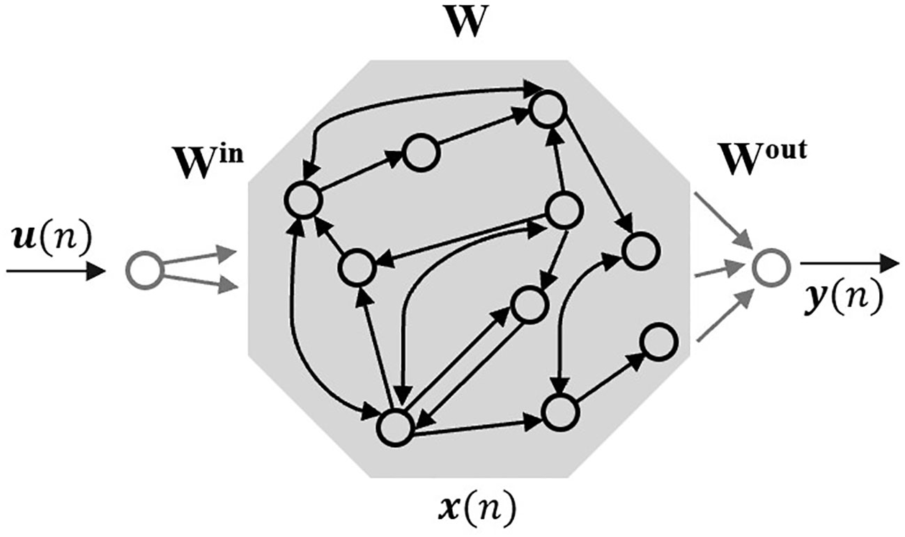
Here, $\mathit{y}(n)$ is the ESN output, and $W^{out}$ is the output weight matrix. The architecture of an ESN is illustrated in Figure 1 (Lukoševičius, 2012). Connections directly from the input units and between output units are allowed (Jaeger, 2001).

Figure 1

Figure 1. Example of an echo state network architecture with one input and one output neuron.

The method of reservoir computing by ESN involves three main steps presented in Jaeger (2001).

1. Generate the reservoir: Construct a large RNN with random recurrent connections, termed the reservoir $(W^{in},W,\alpha )$.

2. Train RNN: Run the RNN using the training input $\mathit{u}(n)$ and collect corresponding reservoir activation states $\mathit{x}(n)$.

3. Use the trained network: Apply the trained network to new input data $\mathit{u}(n)$ with the trained output weights $W^{out}$ to compute the prediction $\mathit{y}(n)$.

3.2.1 Reservoir hyperparameters

The reservoir has to be generated rigorously to implement an ESN with high performance. Key hyperparameters for optimising the ESN reservoir include input scaling, spectral radius, reservoir size and leaking rate. Proper tuning of these parameters is crucial for high performance (Lukoševičius, 2012). Input scaling refers to adjusting the scaling of the input weight matrix Wⁱⁿ to control the reservoir’s nonlinear response. Making the reservoir connections W sparse is also recommended, and the non-zero elements are Gaussian distributed. The spectral radius of the reservoir connection matrix W is denoted as ρ(W). It is the maximum eigenvalue of this matrix, affecting the stability and memory of the reservoir. To ensure stability, the echo state property, ρ(W) < 1, should be selected to maximise the model’s performance. The reservoir size and the number of units in the reservoir influence the model’s capacity to capture input dynamics. Larger reservoirs typically perform better, given appropriate regularisation (Jaeger, 2001; Lukoševičius, 2012).

The most pragmatic way to evaluate a reservoir is by training the output weights using Equation 7 and measuring its error through validation or test error. To ensure deterministic repeatability in experiments, fixing a random seed in the programming environment is crucial for making the random aspects of the reservoir identical over several trials. Automated selection of hyperparameters is preferred for efficiency and reproducibility. When tuning an ESN’s hyperparameters, grid search is the most straightforward option. Implementing a grid search involves nested loops, making it easy to explore a wide range of parameter values. A reasonable approach is to perform a coarser grid search over a wide range, followed by a finer search over more promising parameter ranges. If the best performance in the coarser grid is found at the boundary, the optimal hyperparameters may lie outside the initial grid range. The best choice of hyperparameters is often to average the best parameters in the search. Additionally, plotting some reservoir activation signals $\mathit{x}(n)$ can provide insights into the internal dynamics of the reservoir (Lukoševičius and Uselis, 2019).

3.2.2 Training output weights

ESNs work by linearly combining the input and reservoir units to generate the network output. To find the optimal $W^{out}$ that minimises the RMSE between the output $\mathit{y}(n)$ and the target time series ${\mathit{y}}^{target}(n)$, the ridge regression solution is commonly used and given by Equation 9 where $Y^{target}$ is defined as in Equation 8, the matrix form of Equation 7, I is the identity matrix, and β is the regularisation coefficient. X is here used for notional brevity instead of X = [1;U;X] as a vertical matrix concatenation.

$\begin{array}{ll}{Y}^{target}=W^{out}X& (8)\end{array}$

$\begin{array}{ll}{W}^{out}=Y^{target}{X}^T{(X{X}^T+\beta I)}^{-1}& (9)\end{array}$

Regularisation helps prevent overfitting by adding a penalty to the model’s loss function, maintaining its complexity while ensuring it generalises well to unseen data (Lukoševičius, 2012).

A powerful extension of the basic ESN approach is training many smaller ESNs in parallel and averaging their outputs, $W^{out}$. This reduces the random component of the model output, and in some cases, this approach has drastically improved the ESN model performance (Jaeger et al., 2007).

4 Results

Figures 2, 3 illustrates the decrease in accuracy of respectively ESN and AR models of different order after n-step ahead prediction. For BOSZ data, 1 second into the future corresponds to a one-step ahead prediction. This study aims for a 20-second wave prediction to account for the diminishing accuracy of the models as the prediction horizon extends. After 20 seconds, the AR prediction get out of phase with the data, as the value of the RMSE indicates. The RMSE for models with a prediction horizon longer than 20 seconds is unacceptable high. ESN is more accurate over a longer time horizon with respect to both phase and amplitude as Figure 3 shows. The RMSE (unit meters) for the ESN model is 0.23 after 60 second and is still almost exactly in phase, but for the AR-OLS models the RMSE varies between 0.30 and 0.45, which are unacceptable high in the case of a sea state with a significant wave amplitude of 0.5 meters. However, the AR models capture the first seconds of prediction with higher accuracy on the examined data than ESN overestimates the amplitude. After 20 seconds prediction the AR-OLS models and the prediction with ESN give similar accuracy, respectively RMSE (unit meters) 0.18 and 0.14. By focusing on a 20-second prediction time frame we ensure a fair comparison between AR and ESN, and we aim to capture the wave dynamics precisely.

Figure 2

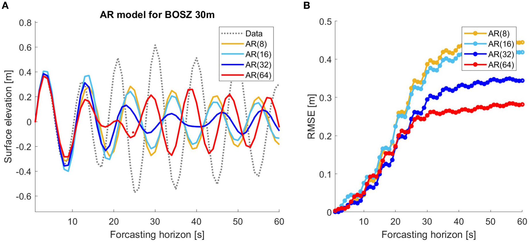
Figure 2. AR models of order 8, 16, 32 and 64 calculated with the OLS method over 60 step ahead prediction corresponds to 60 seconds prediction horizon for BOSZ simulated data at 30 meters depth. (A) Plot of the prediction models (solid lines) and the target signal (dashed line). (B) RMSE (unit: meters) of the AR models after n seconds.

Figure 3

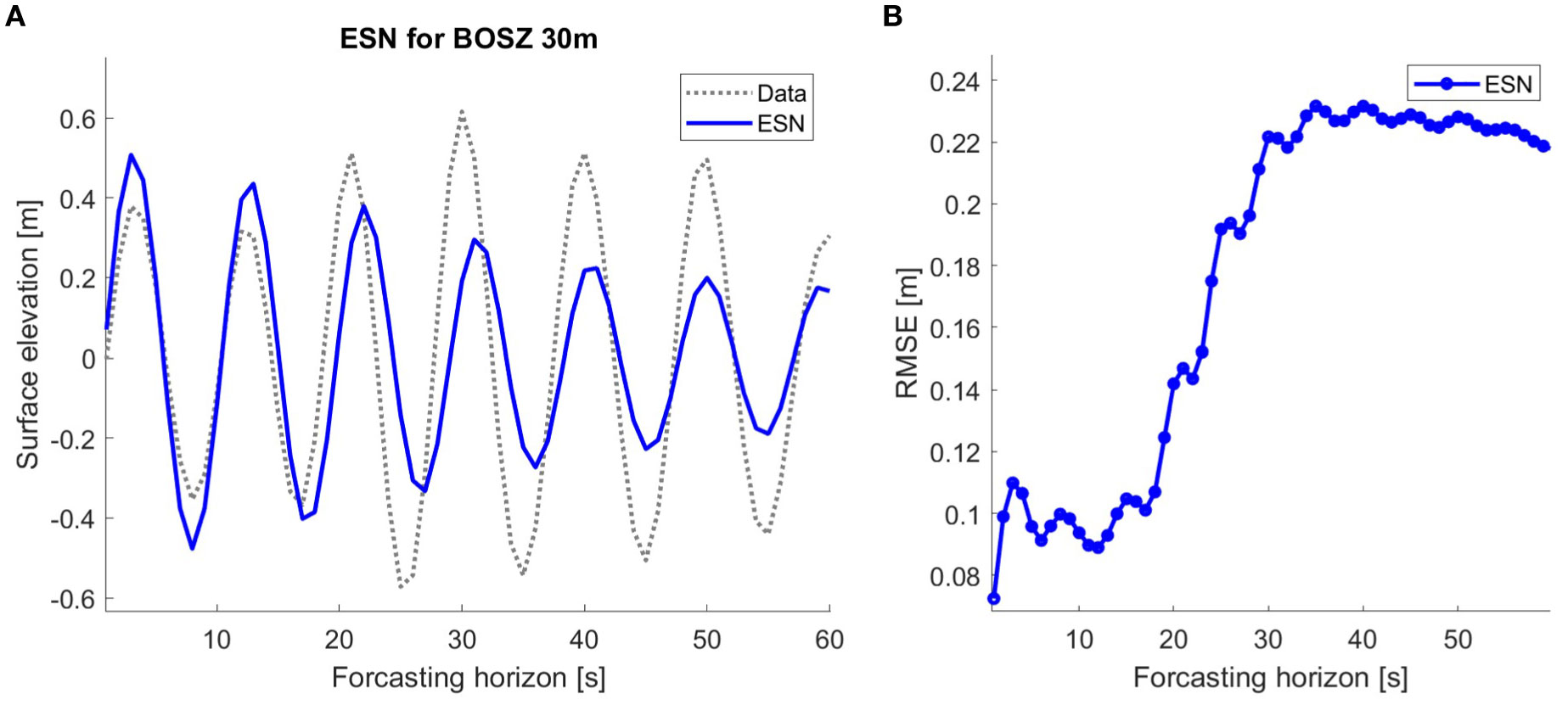
Figure 3. ESN prediction over 60 step ahead prediction corresponds to 60 seconds prediction horizon for BOSZ simulated data at 30 meters depth. (A) Plot of the models (solid lines) and the target signal (dashed line). (B) RMSE (unit: meters) of the ESN prediction after n seconds.

Start by looking at the simulated data, which is essentially low-pass filtered by design. Table 1 presents RMSE for AR models of different orders and ESN for JONSWAP and BOSZ data for a 200-2second prediction length with a 20-second prediction horizon. After every 20 seconds, the AR(p) model takes the last p measurements as new input without recalculating the AR coefficients, and ESN is trained again without calibrating the hyperparameter.

Table 1

Table 1. RMSE (unit: meters) for different AR models and ESN for multi-step ahead prediction for 20 seconds and 10 updates, total prediction length of 200 seconds on simulated data.

The AR coefficients are computed with the standard OLS method for all AR models and compared with the alternative approach, which minimises the multi-step cost function, Equation 3. Here, the Equation 3 is minimised by Gauss Newton’s iteration for a multi-step prediction of 20 seconds (GN-20). All AR models are fitted against a 10-minute wave record training data to approximate the parameters, as this time length gave the most accurate AR coefficients. AR models calculated with GN have lower overall performance; see Table 1. No RMSE was reported for some AR-(GN-20) models of order 64 since the predicted signal “exploded” or the RMSE were unacceptable high. Figure 4 compares the performance of AR(32) for GN-20 and OLS on JONSWAP deep-water data. GN is computationally more expensive and does not yield significantly better results, so AR-GN models will not be considered further. Tables 2, 3 presents RMSE for AR models calculated with OLS and ESN models for real-world data from Bideford Bay at 11 meters depth.

Figure 4

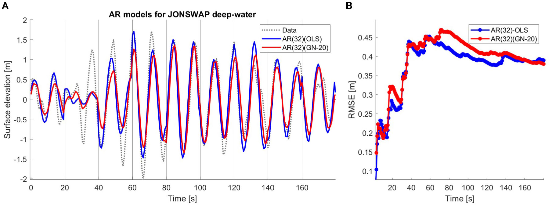
Figure 4. (A) The AR model of order 32 for JONSWAP deep-water computed with the OLS method in blue and computed by minimising Equation 3 with GN-20 in red, and the data in dashed grey. Prediction length of 180 seconds with 20 seconds prediction horizon. (B) RMSE (unit: meters) of AR-OLS (blue) and AR-GN (red) model of order 32 as a function of time for JONSWAP simulated data. Prediction length of 180 seconds with 20 seconds prediction horizon.

Table 2

Table 2. RMSE (unit: meters) for different AR models was calculated with OLS and ESN for multi-step ahead prediction for 20 seconds and 10 updates, total prediction length of 200 seconds on Bidford Bay buoy data at 01/25/2024: T_s = 11.2s, H_s = 2.2m.

Table 3

Table 3. RMSE (unit: meters) for different AR models was calculated with OLS and ESN for multi-step ahead prediction for 20 seconds and 10 updates, total prediction length of 200 seconds on Bidefor Bay buoy data.

The ESN models are trained on as much data as is available for training, leaving 10 minutes for testing to get the possible model performance. The 10-minute testing data is the same dataset used for testing the AR models, so all models are tested on the same wave record and time range. The BOSZ and JONSWAP data are trained on about 100 minutes of wave record. Different lengths of training data, from minutes to hours, are used to train an ESN for Bideford Bay buoy data. In our code, the ESN model is initiated with Gaussian distributed reservoir weights, and 128 units in the reservoir are used. This reservoir size provided the best performance. The ESN models predict the waves’ proper phase, but the amplitude of the waves is generally too low; see Figures 5A, 6. The accuracy of ESN predicting JONSWAP data in Figures 5A, B is lower than expected from Figure 3; but can probably be explained by more varying wave conditions.

Figure 5

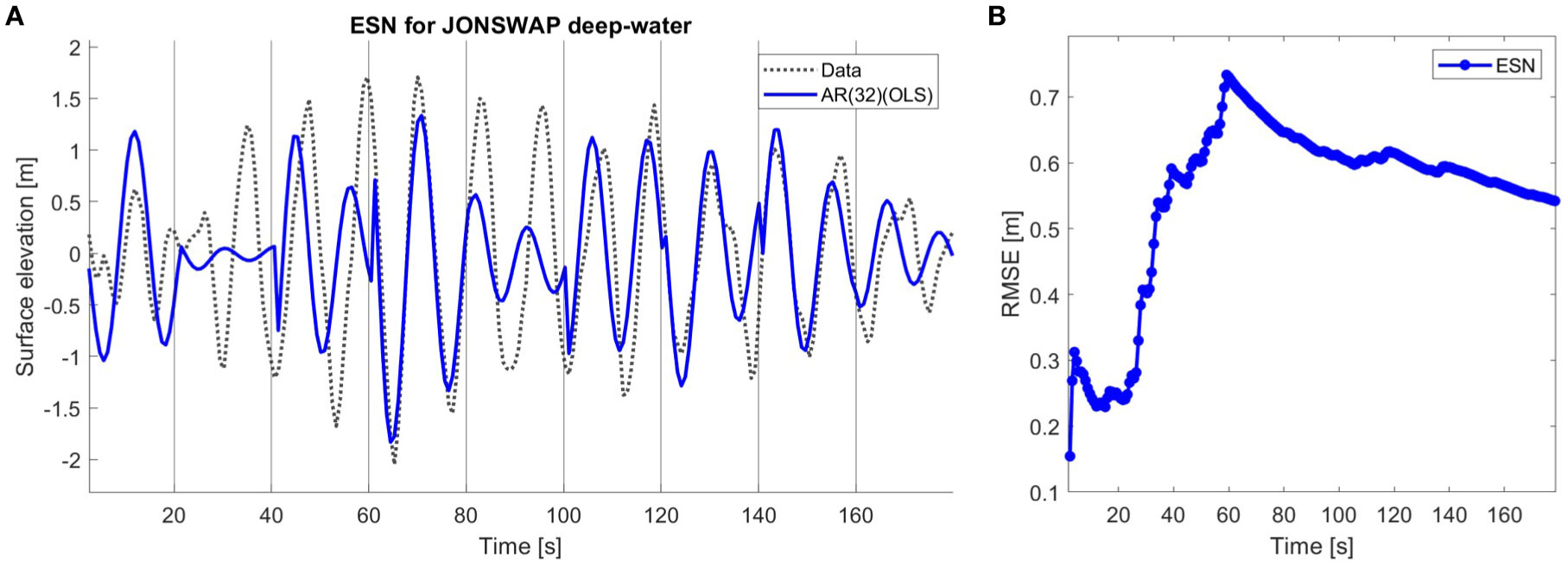
Figure 5. (A) ESN prediction for JONSWAP simulated deep-water data in blue and the data in dashed grey. Prediction length of 180 seconds with 20 seconds prediction horizon. (B) RMSE (unit: meters) as a function of time for ESN prediction JONSWAP data.

Figure 6

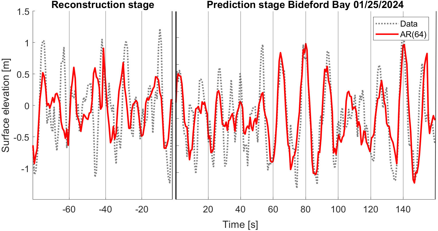
Figure 6. AR(64)-OLS model in red and Bideford Bay buoy data from 01/25/2024 in dashed grey. Sea state: T_s = 11.2s, H_s = 2.2m. The left panel shows 80 seconds of reconstruction stage and the right panel shows 160 seconds of prediction stage with 20-second prediction horizon.

In Table 2, the models are tested on data used for training and compared with unseen data, respectively RMSE_{Reconstruction} and RMSE_Prediction as suggested in Wu et al. (2023). Both prediction and reconstruction length is 200 seconds, and the models updated every 20 second with the last 20-seconds of measurements without updating the model itself. The RMSE are very close in the reconstruction and prediction stage, this ensure overfitting is not present. For the AR models, there is no clear trend between the performance in the reconstruction and prediction stages, see Table 2 and Figure 6. However, the ESN model performs better in the reconstruction part than in the prediction, see Figure 7. Figure 6 compare the prediction of AR(64) model with measurements from Bideford Bay 25 January 2024 and has allover a RMSE (unit meters) of 0.47, and in Figure 7 the ESN prediction in the same case is given with a RMSE of 0.52. As demonstrated in Tables 2 and 3, allover acceptable accuracy for AR-OLS and ESN predicting real-world buoy data from Bideford Bay under different wave conditions.

Figure 7

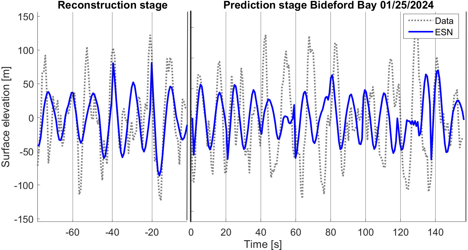
Figure 7. ESN prediction in blue and Bideford Bay buoy data from 01/25/2024 in dashed grey. Sea state: Ts = 11.2s, Hs = 2.2m. The left panel shows 80 seconds of reconstruction stage and the right panel shows 160 seconds of prediction stagewith 20 seconds prediction horizon.

As expected, the performance of the prediction models on field data is lower than the performance of similar models on the simulated data due to the relatively larger share of high-frequency oscillations in the buoy records. Still, the models capture the main surface elevation, which is the low frequencies and the waves with the most energy. The higher-order AR model increases the complexity of the models, and in the case of measurements, it also generalises to unseen data better. Tables 1–5 show that a higher order of the AR model does not necessarily result in higher performance, so the best AR model depends on the complexity of the sea state. The performance of ESN prediction is allover lower, but not significantly lower than for the AR models.

Table 4

Table 4. RMSE (unit: meters) of different AR-OLS models and ESN for multi-step ahead prediction for 20 seconds and 10 updates, total prediction length of 200 seconds on different BOSZ models in 30 meters water depth.

Table 5

Table 5. RMSE (unit: meters) of different AR-OLS models and ESN for multi-step ahead prediction for 20 seconds and 10 updates, total prediction length of 200 seconds on different BOSZ models in 30 meters water depth.

In order to investigate the conditions of the models performance and verify the results of this studyall prediction models are tested on a multiple simulated and measured wave records in intermediate to shallow water for different sea states. The results are shown in Tables 4 and 5. It is evident that data featuring higher significant wave heights have higher lead to larger allover RMSE and for such sea states higher RMSE can still give acceptable results. The overall performance of the models on these datasets, with high significant wave height, is relatively lower than for the wave records with smaller waves. However, it is important to note that the phase is still accurately predicted, and the main cause of the increased error is due to the amplitude. The fact that wave height varies more for sea states with higher waves than for sea states with much shorter waves explains the spread of the reported RMSE for the different models and data. It seems like the wave conditions for BOSZ 5 meters, T_s = 16.6s, H_s = 2.2m, is to dramatic and non-linear for both models for both AR models and ESN to predict with sufficiently high performance. E. g. AR(8) and AR(16) did not capture the wave phase at all. Although predicting the phase of waves at 5 meters of water depth is done with high performance in calmer seas.

5 Real-time control of wave energy converters

In this report, we have seen several models for wave prediction in different water depths, predicting accurately enough to catch the trend in the data. However, are these models robust enough for real-time implementation in WEC applications? The real-time implementation of a phase control system for optimising WECs represents a significant advancement in renewable energy.

The AR model has the potential for real-time implementation for short-time wave prediction in deepwater and intermediate water. In shallow water, as Fusco and Ringwood (2010) proposes, it requires the realisation of a low-pass filter. However, low-pass filtering of historical data does not improve the forecasting results here. As the sea state does not change in the simulated data, it is not surprising that the error estimate does not significantly change for each update interval of 20 seconds over a prediction length of 2 hours. A static AR model for BOSZ 5 meters maintains high accuracy over 2 hours, which is the length of the simulation. As BOSZ is a low-frequency model, we implement a low-pass filter for actual data with high nonlinear components to increase the accuracy of the surface elevation prediction. However, the fact is that implementing a low-pass filter causes a delay, which significantly affects the performance of wave prediction.

Run a real-time implementation of an AR-OLS model of order 32 for 4 hours with a prediction horizon of 20 seconds, in total 720 input updates of the AR model on the Bideford Bay time series. Figure 8 shows RMSE for each prediction window where the red line is the running mean with a filter window of size 3. The mean RMSE (unit meters) over the update windows lies between 0.25 and 0.5 RMSE for 4 hours. The RMSE increases slightly with time as expected, but still after predicting almost four hours the models captures the frequency of the main surface elevation; see Figure 9.

Figure 8

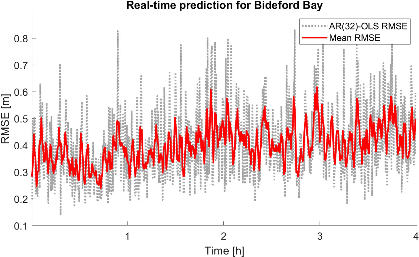
Figure 8. RMSE (unit: meters) of each update-interval in a real-time implementation of AR- OLS model of order 64 for Bideford Bay buoy data in gray and a moving average with a filtering window of 3 points. Prediction length of 4 hours with 20 seconds prediction horizon.

Figure 9

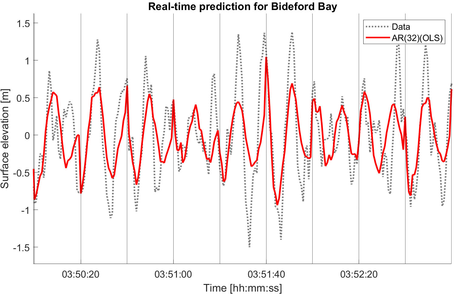
Figure 9. Real-time implementation of AR-OLS model of order 32 for Bideford Bay buoy data. The predicted time series is in red after 3 hours, 50 minutes, and 180 seconds further, with a 20-second prediction horizon.

In a real-time implementation of ESN, we used the same setup as the AR-OLS model for 4 hours with a 20-second prediction horizon, and the results were acceptable. We also did a real-time implementation with a longer prediction horizon, so the output weight was trained more rarely. A 40-second prediction horizon over 4 hours of forecasting gives a mean RMSE (unit meters) over each 40-second prediction window varying between 0.3 and 0.8. As the prediction horizon is twice as long as for the real-time implementation of the AR models, the RMSE is exacted to be higher. However, the RMSE is still and a real-time implementation of ESN is possible as long as the network is trained on enough data, see Figures 10 and 11. The length of the prediction horizon for the considered short-time prediction models depends on the availability of data and the sea conditions as calmer seas are predicted more accurately than more dramatic and non-linear seas.

Figure 10

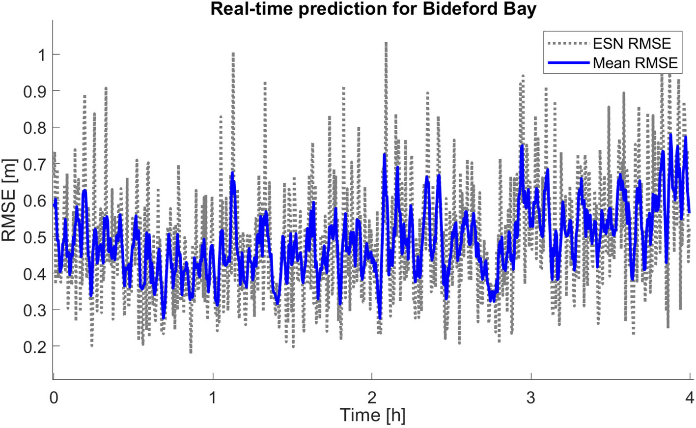
Figure 10. RMSE (unit: meters) of each update-interval in a real-time implementation of the ESN model for Bideford Bay buoy data in grey and a moving average with a filtering window of 3 points in blue. Prediction length of 4 hours with 40 seconds prediction horizon.

Figure 11

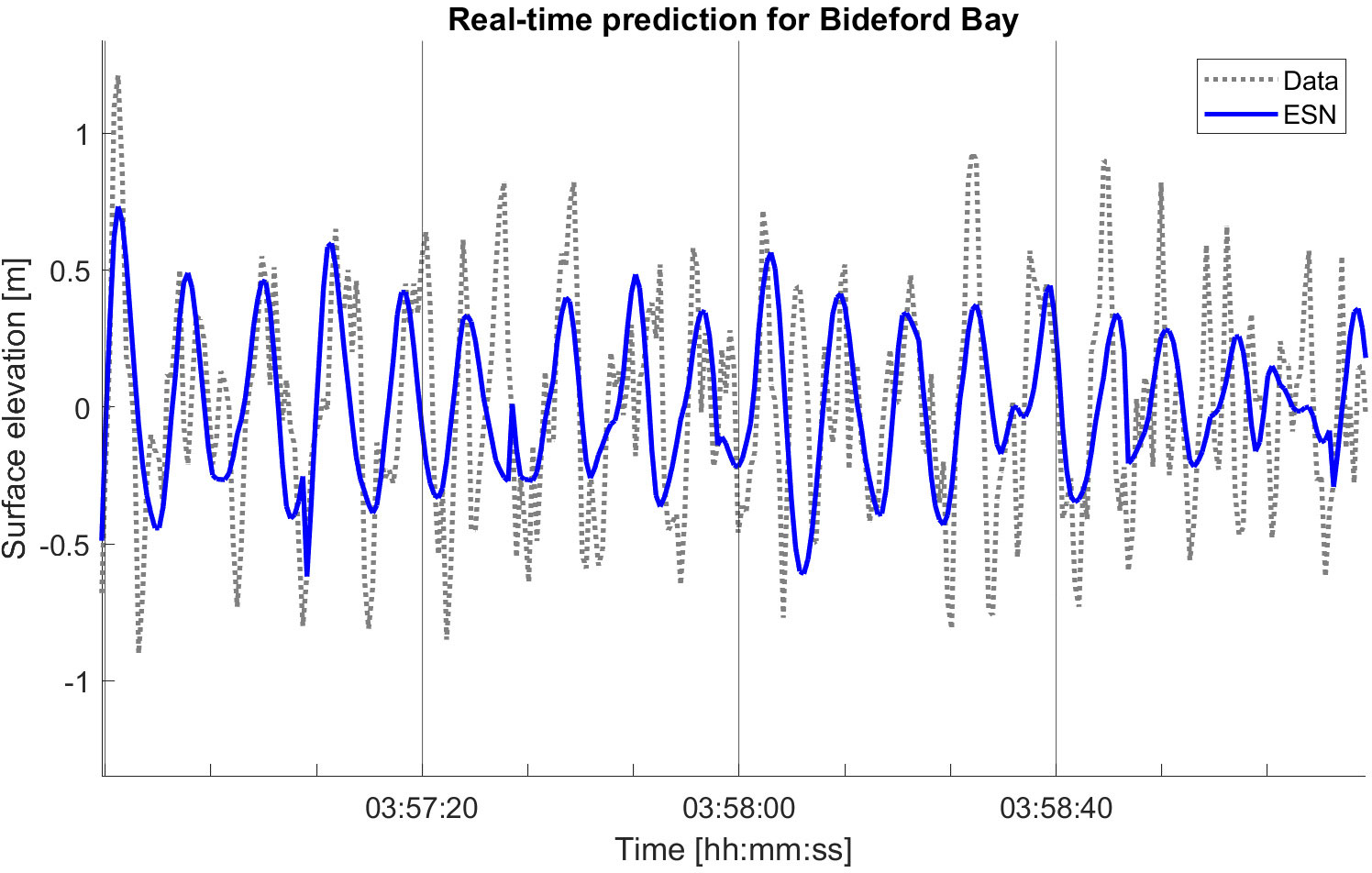
Figure 11. Real-time implementation of ESN for Bideford Bay buoy data. The predicted time series in blue after 3 hours, 56 minutes and 40 seconds, and 160 seconds further, with 40 seconds prediction horizon.

6 Conclusion

In the present contribution, the potential of echo state networks (ESN) and autoregression (AR) for dynamic time series forecasting of ocean waves has been under investigation. The choice of these two methods were partially motivated by the findings of Fusco and Ringwood (2010) which indicated AR as the best overall method among those tested in their work. In particular, it was found that the neural-network approach did not give better results than the AR method. Since the wave signals used in Fusco and Ringwood (2010) were given in deep to intermediate depth, one could ask the question what would happen if waves in shallower water were to be forecast. For wave forecasting in shallow water, an echo state network seems to be a good choice since the architecture is designed to deal with more nonlinear signals (Jaeger and Haas, 2004). In addition to the single output neuron and lean structure that enable fast learning of the network.

According to our investigation, it is possible to accurately predict low-frequency waves for over 4 hours with a 20-second prediction horizon using a model with well-calculated AR coefficients calculated by OLS method. This can be achieved without calibrating the AR coefficients. An Echo State Network can also deliver acceptable results with a similar error as the AR model, but the ESN requires ample data for training. The main advantage of the AR model is its relative simplicity, and it can work effectively with limited access to data for tuning. Thus, we agree with Fusco and Ringwood (2010) that AR models for real-time ocean wave prediction for WECs are a promising approach. They are the most efficient and accurate method for optimising WECs in water depths down to about 10 meters on a prediction horizon of 20 seconds. On the other hand, the ESN model requires significantly more data than the time series we aim to predict. However, the advantage of the ESN model is that if access to a large amount of data is available for training hyperparameters, then the model can make predictions over a longer prediction horizon without recalculating the output weight of the network.

While the ESN mode is inherently a nonlinear model and should have an advantage in shallower depth where the waves are more nonlinear, no clear distinction between the two approaches was observed with regard to performance in the shallowest depth of 5 meters considered here. We also ran some tests with wave data in very shallow water, i.e. in the surf zone using signals also used in Holand et al. (2023). However neither the AR nor the ESN approach were able to give acceptable results for forecasting such signals. Probably the presence of wave breaking makes such predictions too challenging for these relatively simple methods. Of course, from the viewpoint of wave energy extraction, this is not a serious impediment since WECs would most likely not be placed in an area where ample wave breaking is expected due to the large forces on the devices from the breaking waves. If better results are required either with respect to time horizon or shallower depth, one may try to use the ideas of Matysiak et al. (2024), who suggested that the ESN structure may be optimised using ideas from neuroscience, and in particular using the structure of the auditory cortex to build the ESN reservoir.

Data availability statement

Publicly available datasets were analysed in this study. This data can be found here: https://coastalmonitoring.org/realtimedata.

Author contributions

KH: Conceptualization, Formal analysis, Investigation, Methodology, Writing – review & editing, Data curation, Software, Validation, Visualization, Writing – original draft. HK: Conceptualization, Formal analysis, Investigation, Methodology, Writing – review & editing, Funding acquisition, Project administration, Supervision.

Funding

The author(s) declare financial support was received for the research, authorship, and/or publication of this article. University of Bergen, Climate Fund, Green Master Scholarship European Union’s Horizon 2020 research and innovation programme under grant agreement No. 763959. European Union’s Horizon Europe research and innovation programme under the Marie Skłodowska-Curie grant agreement No. 101119437.

Acknowledgments

The authors would like to thank Volker Roeber for providing the simulated data from the BOSZ model which were used in this study.

Conflict of interest

The authors declare that the research was conducted in the absence of any commercial or financial relationships that could be construed as a potential conflict of interest.

Publisher’s note

All claims expressed in this article are solely those of the authors and do not necessarily represent those of their affiliated organizations, or those of the publisher, the editors and the reviewers. Any product that may be evaluated in this article, or claim that may be made by its manufacturer, is not guaranteed or endorsed by the publisher.

Abbreviations

AR, Autoregression; BOSZ, Bossinesq model; ESN, Echo state network; GN, Gauss-Newton iterative method; NNRCMP, National Network of Regional Coastal Monitoring Programmes; RLS, Recursive least square method; RMSE, root mean square error; RNN, recurrent neural networks; OLS, Ordinary least square method; WEC, Wave energy converter.

References

Box E. P., Jenkins G. M., Reinsel G. C. (2008). Time Series Analysis - Forecasting and Control (Hoboken, N.J: John Wiley & Sons).

Google Scholar

Budar K., Falnes J. (1975). A resonant point absorber of ocean-wave power. Nature 256, 478–479. doi: 10.1038/256478a0

Crossref Full Text | Google Scholar

Cervantes L., Kalisch H., Lagona F., Paulsen M., Roeber V. (2021). Statistical wave properties in shallow water using cnoidal theory. Coast. Dynam. 1–9. Available at: http://resolver.tudelft.nl/uuid:4fde3948-0ab7-4ad4-b74f-94b2d3163009.

Google Scholar

Cruz J. (2008). Ocean Wave Energy: Current Status and Future Prespectives (Berlin, Heidelberg: Springer).

Google Scholar

Drew B., Plummer A. R., Sahinkaya M. N. (2009). A review of wave energy converter technology. Proceedings of the Institution of Mechanical Engineers, Part A: Journal of Power and Energy. 223 (8), 887–902. doi: 10.1243/09576509JPE782

Crossref Full Text | Google Scholar

Duan W., Ma X., Huang L., Liu Y., Duan S. (2020). Phase-resolved wave prediction model for long-crest waves based on machine learning. Comput. Methods Appl. Mech. Eng. 372, 113350. doi: 10.1016/j.cma.2020.113350

Crossref Full Text | Google Scholar

Falnes J. (2007). A review of wave-energy extraction. Mar. Struct. 20, 185–201. doi: 10.1016/j.marstruc.2007.09.001

Crossref Full Text | Google Scholar

Falnes J., Kurniawan A. (2020). Ocean waves and oscillating systems: linear interactions including wave-energy extraction Vol. 8 (Cambridge, United Kingdom: Cambridge University Press).

Google Scholar

Fusco F. (2009). Short-term wave forecasting as a univariate time series problem; EE/2009/JVR/03 (Ireland: National University of Maynooth). Technical report.

Google Scholar

Fusco F., Ringwood J. V. (2010). Short-term wave forecasting for real-time control of wave energy converters. IEEE Trans. Sustain. Energy 1, 99–106. doi: 10.1109/TSTE.2010.2047414

Crossref Full Text | Google Scholar

Ge M., Kerrigan E. C. (2016). “Short-term ocean wave forecasting using an autoregressive moving average model,” in 2016 UKACC 11th International Conference on Control (CONTROL 2016), Vol. 1–6 (Piscataway, New Jersey, United States: IEEE). doi: 10.1109/CONTROL.2016.7737594

Crossref Full Text | Google Scholar

Holand K., Kalisch H., Bjørnestad M., Streßer M., Buckley M., Horstmann J., et al. (2023). Identification of wave breaking from nearshore wave-by-wave records. Phys. Fluids 35, 092105–1–092105–9. doi: 10.1063/5.0165053

Crossref Full Text | Google Scholar

Jaeger H. (2001). The “echo state” approach to analysing and training recurrent neural networks (St. Augustin. Germany: German National Research Center for Information Technology). Technical Report GMD Report 148.

Google Scholar

Jaeger H., Haas H. (2004). Harnessing nonlinearity: Predicting chaotic systems and saving energy in wireless communications. Science 304, 78–80. doi: 10.1126/science.1091277

PubMed Abstract | Crossref Full Text | Google Scholar

Jaeger H., Lukoševičius M., Popovici D., Siewert U. (2007). Optimization and applications of echo state networks with leaky-integrator neurons. Neural Networks 20, 335–352. doi: 10.1016/j.neunet.2007.04.016

PubMed Abstract | Crossref Full Text | Google Scholar

Kagemoto H. (2020). Forecasting a water-surface wave train with artificial intelligence- a case study. Ocean Eng. 207, 107380. doi: 10.1016/j.oceaneng.2020.107380

Crossref Full Text | Google Scholar

Laporte Weywada P., Scriven J., Matysiak A., König R., May P., Roeber V., et al. (2021). “Performance vs. survivability: Evaluation of a range of control strategies in a 1MW oscillating wave surge converter (OWSC),” in EWTEC 2021. Proceedings of the European Wave and Tidal Energy Conference. (Southampton, UK: University of Southampton) 14.

Google Scholar

Liu D., Shah S. L., Fisher D. G. (1999). “Multiple prediction models for long range predictive control, IFAC Proceedings. 32 Amsterdam: Elsevier(2), pp.6775–6780.

Google Scholar

Lukoševičius M. (2012). “A practical guide to applying echo state networks,” in Neural Networks: Tricks of the Trade, 2nd ed. Eds. Montavon G., Orr G. B., Müller K.-R. (Springer, Berlin, Heidelberg), 659–686.

Google Scholar

Lukoševičius M., Uselis A. (2019). “Efficient cross-validation of echo state networks,” in Artificial Neural Networks and Machine Learning – ICANN 2019: Workshop and Special Sessions. Eds. Tetko I. V., Kůrková V., Karpov P., Theis F. (Springer International Publishing, Cham), 121–133.

Google Scholar

Ma X., Huang L., Duan W., Jing Y., Zheng Q. (2021). The performance and optimization of ann-wp model under unknown sea states. Ocean Eng. 239, 109858. doi: 10.1016/j.oceaneng.2021.109858

Crossref Full Text | Google Scholar

Matysiak A., Roeber V., Kalisch H., König R., May P. J. (2024). Listen to the waves: Using a neuronal model of the human auditory system to predict ocean waves. arXiv. 2024, 1–23. doi: 10.48550/arXiv.2404.095105

Crossref Full Text | Google Scholar

Meng Z., Chen Z., Khoo B., Zhang A. (2022). Long-time prediction of sea wave trains by lstm machine learning method. Ocean Eng. 262, 112213. doi: 10.1016/j.oceaneng.2022.112213

Crossref Full Text | Google Scholar

NNRCMP (2024). Bideford bay 1 Hz data for 25/01/2024 10:00 GMT (United Kingdom: National Network of Regional Coastal Monitoring Programmes).

Google Scholar

Ringwood J. V., Bacelli G., Fusco F. (2014). Energy-maximizing control of wave-energy converters: The development of control system technology to optimize their operation. IEEE Control Syst. Mag. 34, 30–55. doi: 10.1109/MCS.2014.2333253

Crossref Full Text | Google Scholar

Roeber V., Cheung K. F., Kobayashi M. H. (2010). Shock-capturing Boussinesq-type model for nearshore wave processes. Coast. Eng. 57, 407–423. doi: 10.1016/j.coastaleng.2009.11.007

Crossref Full Text | Google Scholar

Wu J., Xiao D., Luo M. (2023). Deep-learning assisted reduced order model for high-dimensional flow prediction from sparse data. Phys. Fluids 35, 103115. doi: 10.1063/5.0166114

Crossref Full Text | Google Scholar

Yevnin Y., Chorev S., Dukan I., Toledo Y. (2023). Short-term wave forecasts using gated recurrent unit model. Ocean Eng. 268, 113389. doi: 10.1016/j.oceaneng.2023.113389

Crossref Full Text | Google Scholar