ISSA optimized spatiotemporal prediction model of dissolved oxygen for marine ranching integrating DAM and Bi-GRU

In marine ranching aquaculture, dissolved oxygen (DO) is a crucial parameter that directly impacts the survival, growth, and profitability of cultured organisms. To effectively guide the early warning and regulation of DO in aquaculture waters, this study proposes a hybrid model for spatiotemporal DO prediction named PCA-ISSA-DAM-Bi-GRU. Firstly, principal component analysis (PCA) is applied to reduce the dimensionality of the input data and eliminate data redundancy. Secondly, an improved sparrow search algorithm (ISSA) based on multi strategy fusion is proposed to enhance the optimization ability and convergence speed of the standard SSA by optimizing the population initialization method, improving the location update strategies for discoverers and followers, and introducing a Cauchy-Gaussian mutation strategy. Thirdly, a feature and temporal dual attention mechanism (DAM) is incorporated to the baseline temporal prediction model Bi-GRU to construct a feature extraction network DAM-Bi-GRU. Fourthly, the ISSA is utilized to optimize the hyperparameters of DAM-Bi-GRU. Finally, the proposed model is trained, validated, and tested using water quality and meteorological parameter data collected from a self-built LoRa+5G-based marine ranching aquaculture monitoring system. The results show that: (1) Compared with the baseline model Bi-GRU, the addition of PCA, ISSA and DAM module can effectively improve the prediction performance of the model, and their fusion is effective; (2) ISSA demonstrates superior capability in optimizing model hyperparameters and convergence speed compared to traditional methods such as standard SSA, genetic algorithm (GA), and particle swarm optimization (PSO); (3) The proposed hybrid model achieves a root mean square error (RMSE) of 0.2136, a mean absolute percentage error (MAPE) of 0.0232, and a Nash efficient (NSE) of 0.9427 for DO prediction, outperforming other similar data-driven models such as IBAS-LSTM and IDA-GRU. The prediction performance of the model meets the practical needs of precise DO prediction in aquaculture.

1 Introduction

As one of the crucial indicators of water quality, dissolved oxygen directly determines the health status of the water environment in marine ranching, and then affects the overall aquaculture benefits. Its concentration is influenced by factors such as air temperature, atmospheric pressure, and water body conditions, exhibiting nonlinear, coupled, and time-varying characteristics (Cuenco et al., 1985; Lipizer et al., 2014). When the DO concentration in water is too high or insufficient, it can directly or indirectly alter other water quality indicators, affecting the health status of aquacultured species, leading to decreased resistance, slow growth, stagnation, or even death (Abdel-Tawwab et al., 2019; Neilan and Rose, 2014; Jiang et al., 2021). Therefore, through real-time monitoring and effective prediction of DO concentration in water aquaculture, precise regulation of the water quality environment can be achieved, reducing the aquaculture risks in marine farms and enhancing their economic benefits.

Currently, artificial intelligence technology is widely used for modeling complex nonlinear systems (Zhu et al., 2019; Choi et al., 2021; Than et al., 2021; Guo et al., 2022, 2023). Scholars have proposed various methods for water quality prediction in different environments and achieved certain results. Wu et al. (2018) used a BP neural network model optimized by particle swarm optimization (PSO) for dissolved oxygen prediction. Zhu et al. (2017) established a dissolved oxygen prediction model based on the least squares support vector regression (LSSVR) model and fruit fly optimization algorithm (FOA). Li et al. (2023) applied a prediction model combining PCA with particle swarm optimization-based LSSVM to dissolved oxygen prediction in the Yangtze River Basin in Shanghai. Kuang et al. (2020) proposed a hybrid DO prediction model KIG-ELM consisting of K-means, improved genetic algorithm (IGA), and extreme learning machine (ELM). Cao et al. (2021a) proposed a method based on k-means clustering, PSO, and an improved soft ensemble extreme learning machine (SELM). The BP, SVM, LSSVM, and ELM prediction methods mentioned above all belong to shallow machine learning models. They have fast training speeds and can achieve high accuracy, but their representation capabilities for complex functions are limited under limited samples and computing units. Their generalization ability for complex classification problems is also constrained to a certain extent.

Additionally, scholars have also proposed an adaptive network-based fuzzy inference system (ANFIS), which combines the characteristics of fuzzy logic and neural networks. By learning the fuzzy rules and weight parameters from data, ANFIS can predict unknown data. Sharad et al. (2018) introduced two data-driven adaptive neuro-fuzzy systems: fuzzy C-means and ANFIS based on subtractive clustering, which were used to predict sensitive parameters in monitoring stations that could lead to changes in existing water quality index values. Arora and Keshari (2021) employed ANFIS with grid partitioning (ANFIS-GP) and subtractive clustering (ANFIS-SC) to simulate and predict high-dimensional river characteristics. The results showed that both ANFIS models could fully and accurately predict DO. However, ANFIS lacks adaptability, precise control over complex systems, and may encounter high computational complexity when dealing with complex problems.

In recent years, the development of deep learning models has provided an effective solution for the prediction of dissolved oxygen in aquaculture. Deep learning can achieve complex function approximation by learning a deep nonlinear network structure and mine the implicit information in data. Compared with machine learning methods with shallow structures, it has stronger learning and generalization abilities and demonstrates a strong ability to learn the essential features of data sets from a small number of samples. Among them, the recurrent neural network (RNN) based on deep learning, as a powerful tool for modeling sequential data, has received widespread attention and application. By introducing a recurrent structure within the network, RNN can model the temporal dependencies in sequential data, thereby capturing temporal dependencies and contextual information. However, due to parameter sharing and multiple multiplications, RNN is prone to the problems of gradient vanishing or gradient explosion during backpropagation, making it difficult to train the model or causing it to fail to converge. Long short-term memory (LSTM) and gated recurrent unit neural network (GRU), as the most popular variants of RNN, can effectively address the issues of gradient vanishing and gradient explosion during RNN training, and have become the mainstream for time series prediction (Li et al., 2021; Liu P. et al., 2019). Compared to LSTM, GRU consists of an update gate and a reset gate with simpler structure and fewer number of hyperparameters. Liu Y. et al., (2019) conducted research on short-term and long-term DO predictions using attention-based RNN, indicating that the proposed model outperformed five attention-based RNN methods and five baseline methods. Zhang et al., 2020 introduced a DO prediction model, kPCA-RNN, which combines Kernel PCA and RNN demonstrating that the model’s prediction performance surpassed current feedforward neural networks (FFNNs), support vector regression (SVR), and general regression neural networks (GRNN). Sun et al., 2021 proposed a DO prediction model that integrates an improved beetle antennae search algorithm (IBAS) with LSTM networks. Cao et al. (2021b) proposed a LSTM prediction model based on K-means clustering and improved particle swarm optimization (IPSO). Huan et al., 2022 systematically discussed and compared GRU water quality prediction methods based on the attention mechanism. The results showed that its performance in DO prediction surpassed that of LSTM based on the attention mechanism, as well as five traditional baseline algorithms: ANFISR, BF-AN, ELM, SVR, and ANN. However, only the feature attention mechanism was utilized in their study. Chen et al. (2022) established an attention-based LSTM model (AT-LSTM) to predict water quality in the Burnett River in Australia. The research findings indicated that the incorporation of the attention mechanism enhanced the prediction performance of the LSTM model. Only the temporal attention mechanism was used in their study. Tan et al. (2022) constructed a neural network model combining CNN and LSTM to predict DO demonstrating that this model achieved more accurate peak fitting predictions than traditional LSTM models. Yang and Liu (2022) utilized an improved whale optimization algorithm (IWOA) to optimize a GRU, creating a water quality prediction model for sea cucumber aquaculture. Experimental results showed that this model surpassed prediction models such as Support Vector Regression (SVR), Random Forest (RF), CNN, RNN, and LSTM networks in terms of prediction accuracy and generalization performance. Jiange et al. (2023) proposed a prediction model combining improved grey relational analysis (IGRA) with LSTM optimized by the ISSA named IGRA-ISSA-LSTM. Results indicated that the proposed model achieved higher determination coefficients (R2) for predicting DO, pH, and KMnO4 compared to the IGRA-BP, IGRA-LSTM, and IGRA-SSA-LSTM models. Zhang et al. (2023) introduced an DO spatio-temporal prediction model based on an improved RGU with a dual attention mechanism (IDA-GRU) and an improved inverse distance weighting (IIDW) interpolation algorithm.

Existing research has shown that various models can be employed for DO prediction, with deep learning-based models outperforming shallow machine learning models and ANFIS. The critical aspects of building an efficient and accurate DO prediction model focus on preprocessing of input data, model selection and improvement and hyperparameter optimization (Wang et al., 2023). Based on these findings, this paper proposes an hybrid model, named PCA-ISSA-DAM-Bi-GRU, to predicting DO in marine aquaculture farms. Specifically, PCA is utilized for dimensionality reduction of the model input data, while the DAM integrating both temporal and feature attention, is fused with the bidirectional gated recurrent unit (Bi-GRU) neural network for feature extraction. Furthermore, an enhanced ISSA incorporating multiple strategies is employed to search and optimize the hyperparameters of the Bi-GRU, aiming to enhance the model’s prediction precision. Finally, the accuracy and reliability of the model are validated using data collected from a self-built LoRa+5G-based marine aquaculture farm monitoring system.

2 Materials and methods

2.1 Marine ranching environment monitoring system based on LoRa+5G

This experiment has independently established a marine ranching environment monitoring system based on LoRa+5G, which integrates functions such as data collection, remote transmission, storage management, remote monitoring, and data analysis. The overall architecture is shown in Figure 1 and can be functionally divided into a perception layer, a network layer, and an application layer. The perception layer utilizes various sensors to collect water quality parameters and meteorological parameters. The network layer transmits the collected data to the application layer through the LoRa sensor network combined with 5G communication technology. The application layer stores and analyzes the collected data, providing a user interface as needed.

Figure 1

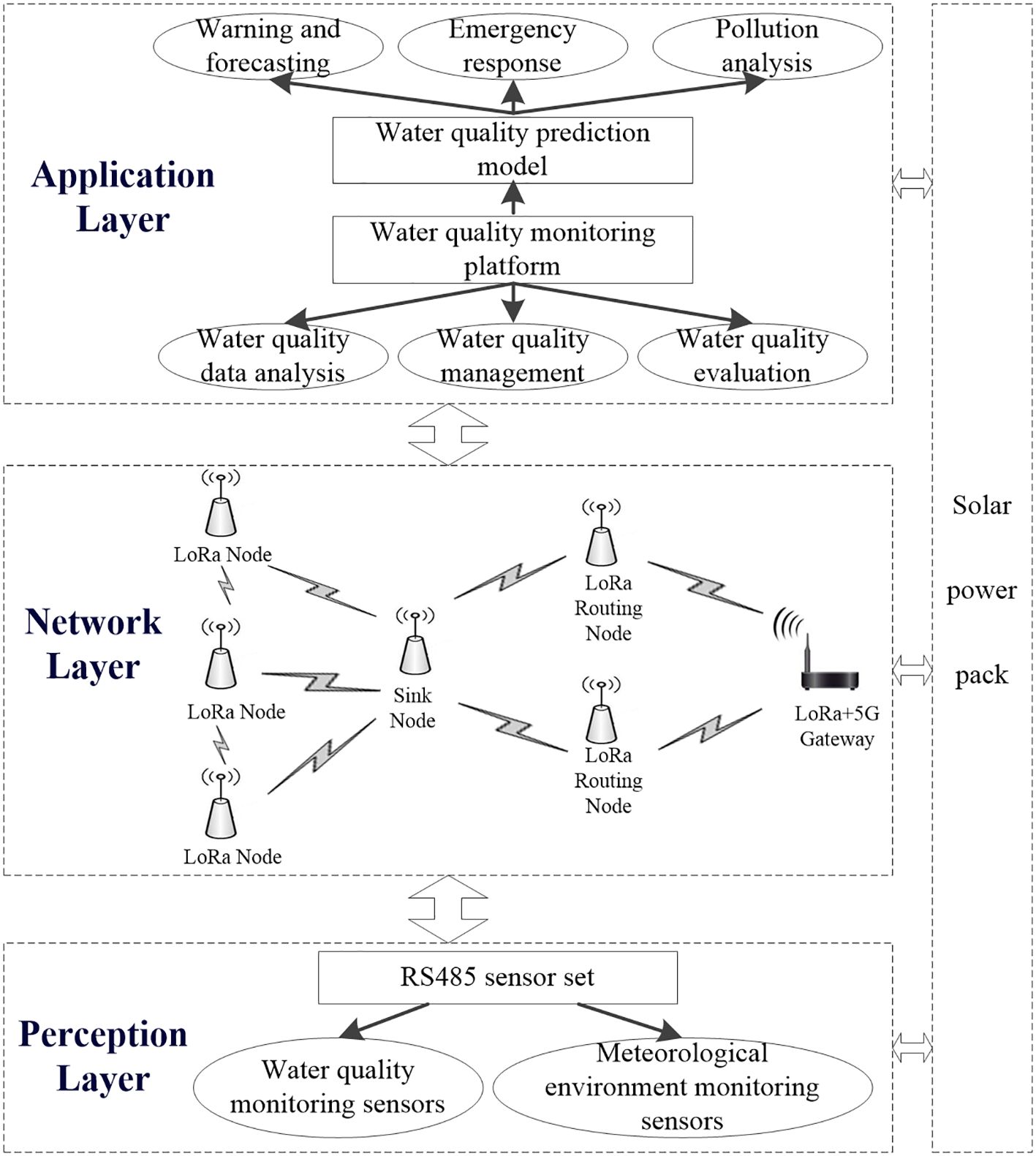
Figure 1. Overall structure of the aquaculture environmental monitoring system.

For this experiment, the monitoring system was deployed at an aquaculture farm in Xiayang Town, Xuwen County, Zhanjiang City, Guangdong Province, China, covering a sea area of 40m in length and 40m in width. To collect three-dimensional distribution data of the aquaculture area, nine water quality sensors were placed at corresponding locations above and below water depths of 0.8m and 1.6m. The monitor point distribution is shown in Figure 2.

Figure 2

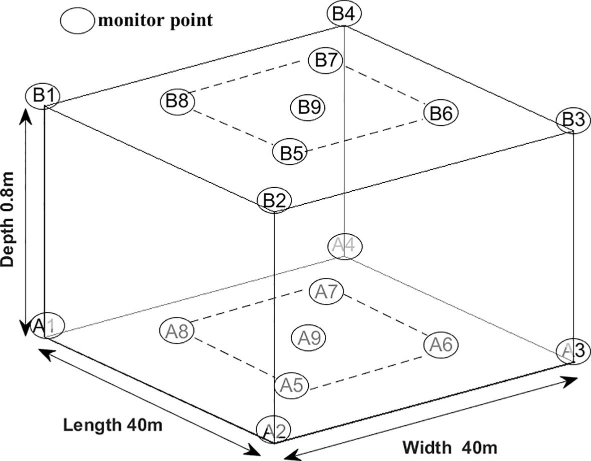
Figure 2. The distribution of monitor points.

The data collected by the water quality sensors include dissolved oxygen, water temperature, conductivity, pH value, ammonia nitrogen content, and turbidity. The meteorological monitoring station, located near the aquaculture farm, gathers data on atmospheric temperature, atmospheric relative humidity, atmospheric pressure, wind speed, wind direction, solar radiation, and rainfall. During the data collection process, factors such as the aquaculture environment, sensor malfunctions, and fluctuations in network signals can lead to the presence of abnormal values and a small number of missing values in the sample data. In this study, the mean smoothing method is adopted to eliminate abnormal data, and the linear interpolation method is used to fill in missing values. Additionally, a min-max normalization process is applied to each variable to ensure consistent scaling for analysis.

2.2 Construction of dissolved oxygen prediction model

2.2.1 Principal component analysis

On the basis of ensuring the integrity, validity, and accuracy of the input data, dimensionality reduction can be applied to eliminate redundancy in the input data, effectively reduce the complexity of the model structure, and enhance the model’s learning performance and prediction accuracy. Principal Component Analysis (PCA) is a commonly used data analysis method that transforms data from a high-dimensional space to a low-dimensional space. It recombines numerous indicators with certain correlations into a new set of uncorrelated comprehensive indicators, thereby achieving the goals of removing redundant information and noise reduction. Assuming the input raw data is in the form of a matrix, the specific steps for PCA to extract the principal components are as follows:

1. Data Decentralization: subtract the mean of each feature from itself ${X^{\prime }}_{ij}=X_{ij}-{\overline{X}}_i$;

2. Compute the Covariance Matrix: ${X^{\prime }}_{ij}{X^{\prime T}}_{ij}$;

3. Calculate Eigenvalues and Eigenvector;

4. Select Principal Components: sort the eigenvalues from largest to smallest and select the top k eigenvalues;

5. Construct Projection Matrix: combine the eigenvectors corresponding to the selected eigenvalues to form the projection matrix;

6. Dimensionality Reduction: multiply the original matrix by the projection matrix to obtain a new set of samples that retains most of the representative feature information from the original samples.

2.2.2 Bi-directional gated recurrent unit neural network

The GRU network is a simplified variant of the LSTM network. It consists of an update gate and a reset gate, resulting in a simpler structure with fewer hyperparameters. GRU networks take sequential data as input and utilize recurrent convolutional neural networks for feature extraction, making them well-suited for time series prediction. The specific structure of the GRU network cycle unit is illustrated in Figure 3. The input of the network unit includes the current input x_t and the hidden state h_t-1 passed down from the previous time step. The output is both the output for the current time step and the hidden state h_t passed to the next time step. The specific calculation process is described by Equations 1–4:

Figure 3

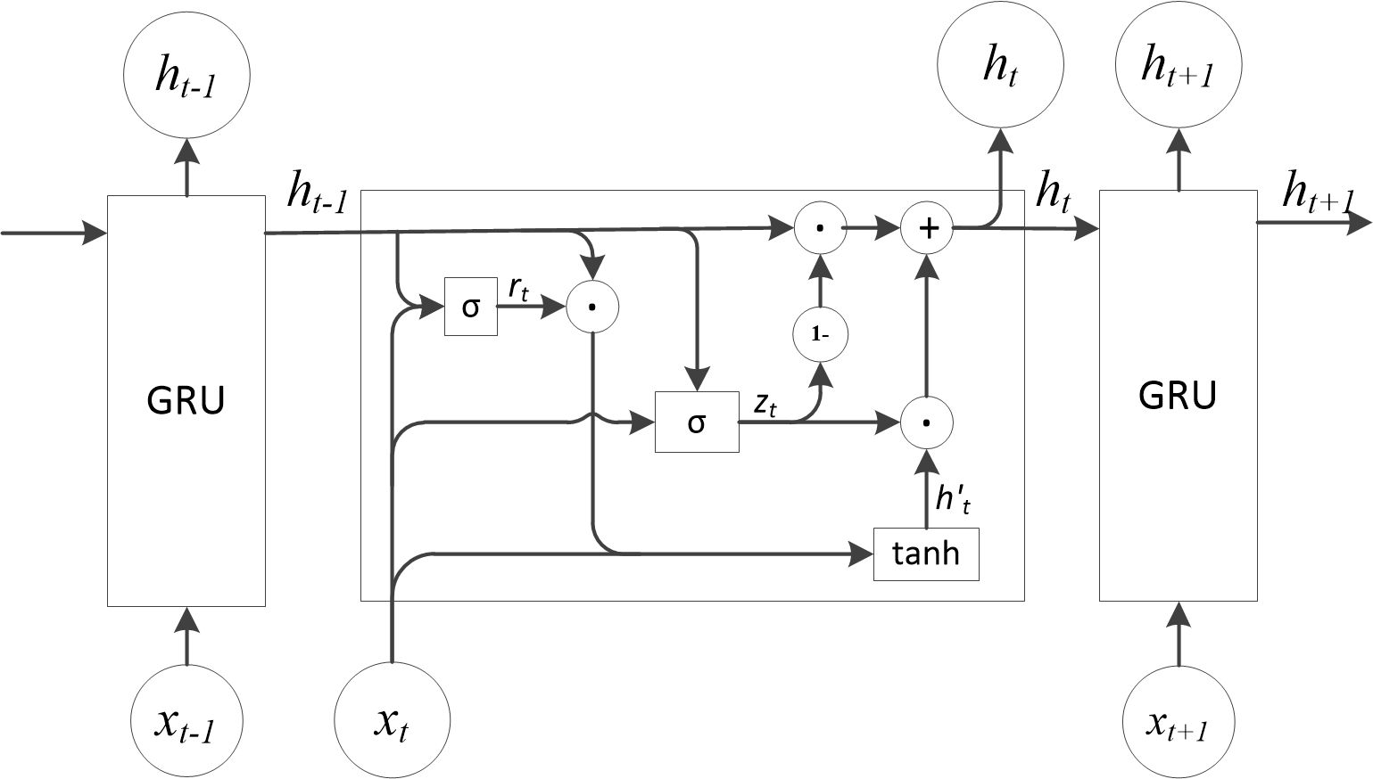
Figure 3. Basic structure of GRU.

$\begin{array}{ll}{r}_t=\sigma (W_{rx}{x}_t+W_{rh}{h}_{t-1}+b_r)& (1)\end{array}$

$\begin{array}{ll}{z}_t=\sigma (W_{zx}{x}_t+W_{zh}{h}_{t-1}+b_z)& (2)\end{array}$

$\begin{array}{ll}{h}_t^{\text{'}}=\tanh (W_{hx}{x}_t+W_{hr}{r}_t{h}_{t-1}+b_h)& (3)\end{array}$

$\begin{array}{ll}{h}_t=(1-z_t)h_{t-1}+z_t{h}_t^{\text{'}}& (4)\end{array}$

where $r_t$, $z_t$, $h_t^{\text{'}}$ and $h_t$ represent the output of the reset gate, the output of the update gate, the candidate state, and the hidden state, respectively. $W_{rx}$ and $W_{rh}$ are the weight matrices of the reset gate, $W_{zx}$ and $W_{zh}$ are the weight matrices of the update gate, and $W_{hx}$ and $W_{hr}$ are the weight matrices of the candidate output. $b_r$, $b_z$ and $b_h$ are the bias vectors for the reset gate, the update gate, and the candidate output, respectively. $\sigma$ and $\text{tanh}$ denote the sigmoid activation function and the hyperbolic tangent function, respectively.

Since GRU can only establish unidirectional associations in time series, the concentration of dissolved oxygen at a given moment should be related to both the preceding and following water quality and meteorological factors. The bidirectional GRU (Bi-GRU) can simultaneously mine the sequential correlation and reverse correlation of the time series, and comprehensively extract the timing features. Therefore, this study employs bi-directional GRU (Bi-GRU), which simultaneously explores the sequential and inverse sequential correlations in the time series, comprehensively extracting temporal features. The Bi-GRU network comprises two independently and symmetrically structured GRUs with identical inputs but opposite information transmission directions. The outputs from these two GRUs, which are independent and do not interact with each other, are concatenated to form the output for each time step, as shown in Figure 4.

Figure 4

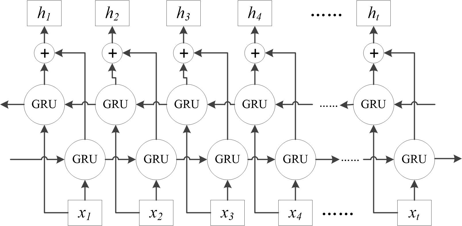
Figure 4. Bi-GRU network structure.

2.2.3 Dual attention mechanism

The attention mechanism in deep learning is a biomimetic technique that mimics the selective attention behavior in human reading, listening and speaking. Integrating attention mechanisms into neural network can make it autonomously learn and pay more attention to the important information in model input, and enhances the model’s feature extraction capabilities, robustness, and generalization ability by assigning different weights to the model’s inputs. In the DO prediction, the importance of each environmental factor is different, and the influence weight of the same environmental factor on DO concentration at different time points is also different. Furthermore, environmental factors at different historical moments have different importance in influencing current DO concentrations. Therefore, in this study, a feature attention mechanism is introduced at the Bi-GRU encoder stage to adaptively assign weights to different environmental factors at each time step. This mechanism enables the model to focus on the most influential factors for DO prediction. Additionally, a temporal attention mechanism is introduced at the decoder stage of the fully connected layer to dynamically adjust the weights of different time steps’ influence on the current DO concentration, so as to better capture the key information in the time series data. The combination of these two attention mechanisms allows for a more comprehensive and nuanced understanding of the complex relationships between environmental factors and DO concentrations over time.

The feature attention mechanism in the encoder utilizes multi-layer perceptron operations to quantify the feature attention weights, as illustrated in Figure 5. Its input comprises n environmental feature vectors $x_t=(x_t^1,x_t^2,\cdots ,x_t^n)$ at time t and the hidden layer state h_t-1 output by the encoder at the previous time step. The output is the attention weight of each feature at this time step ${\alpha }_t=({\alpha }_t^1,{\alpha }_t^2,\cdots ,{\alpha }_t^n)$, where ${\alpha }_t^k$ assesses the importance of the k-th feature. Subsequently, the updated ${\tilde{x}}_t=({\alpha }_t^1{x}_t^1,{\alpha }_t^2{x}_t^2,\cdots ,{\alpha }_t^n{x}_t^n)$ is employed as the encoder input for time t. The specific calculation process is outlined in Equations 5 and 6:

Figure 5

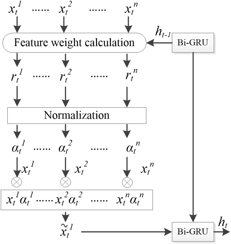
Figure 5. Structural diagram of the feature attention mechanism.

$\begin{array}{ll}{r}_t^k=V_r^T\tanh (W_r{h}_{t-1}+U_r{x}^k+b_r)& (5)\end{array}$

$\begin{array}{ll}{\alpha }_t^k=\text{softmax}(r_t^k)=\frac{\exp (r_t^k)}{{\displaystyle \sum _{i=1}^n\exp (r_t^i)}}& (6)\end{array}$

where $V_r^T$, $W_r$ and $U_r$ represents the network feature weights that need to be learned, and $b_r$ is the bias parameters. The softmax function is applied for normalization, ensuring that the sum of all weights equals 1.

The temporal attention mechanism structure in the decoder is illustrated in Figure 6. Take the encoder’s historical hidden state $H=(h_1^{},\cdots ,h_t^{}\cdots ,h_T^{})$ and the decoder’s hidden layer state at the previous moment d_t-1 as the input of the temporal attention mechanism to obtain the temporal attention weight coefficient ${\beta }_t=({\beta }_t^1,{\beta }_t^2,\cdots ,{\beta }_t^T)$ at the current moment. ${\beta }_t^k$ represents the influence of the hidden layer state at the k-th layer on the DO prediction at the current moment. By weighted summing the ${\beta }_t^k$ with the corresponding hidden layer state $h_k$, the comprehensive information of the predicted time series features could be obtained:. The calculation process is shown in Equations 7 and 9:

Figure 6

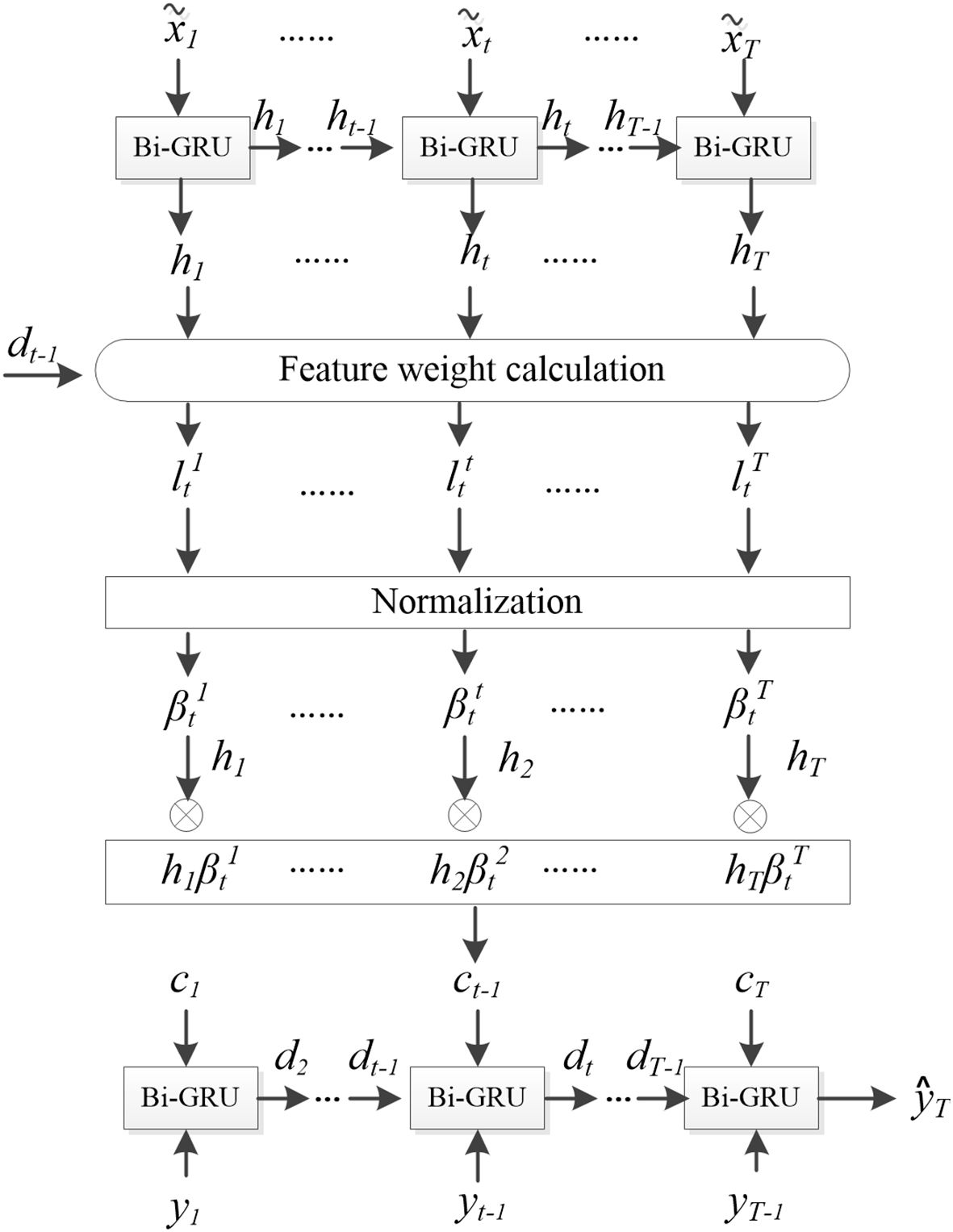
Figure 6. Structural diagram of the temporal attention mechanism.

$\begin{array}{ll}{l}_t^k=V_d^T\tanh (W_d{d}_{t-1}+U_d{h}_k+b_d)& (7)\end{array}$

$\begin{array}{ll}{\beta }_t^k=\text{softmax}(l_t^k)=\frac{\exp (l_t^k)}{{\displaystyle \sum _{i=1}^T\exp (l_t^i)}}& (8)\end{array}$

$\begin{array}{ll}{c}_t={\displaystyle \sum _{k=1}^t{\beta }_t^k}{h}_k& (9)\end{array}$

where $V_d^T$, $W_d$ and $U_d$ represents the network feature weights that need to be learned, and $b_d$ is the bias parameters. The softmax function is applied for normalization, ensuring that the sum of all weights equals 1.

Fuse the dissolved oxygen yt with ct as the input to the GRU network:

$\begin{array}{ll}{\tilde{y}}_t={\tilde{W}}^T[y_t,c_t]+\tilde{b}& (10)\end{array}$

where ${\tilde{\mathit{W}}}^T$ and $\tilde{b}$ represents the weights and biases for the fused input to the GRU neural network.

The hidden state after incorporating the temporal attention mechanism is updated using Equation 11:

$\begin{array}{ll}{d}_t=f_1(d_{t-1},{\tilde{y}}_{t-1})& (11)\end{array}$

The predicted value of the dissolved oxygen to be predicted is:

$\begin{array}{ll}{\tilde{y}}_{T+1}=F(y_1,y_2,\dots y_T,x_1,x_2,\dots x_T)=V_y^T(W_y[d_T,c_T]+b_w)+b_y& (12)\end{array}$

where $W_y$ and $b_w$ are the weights and biases of the GRU network, respectively; while $V_y^T$ and $b_y$ are the weights and biases of the entire network, respectively.

2.2.4 Improved sparrow search algorithm

The hyperparameters of neural network models affect the structure, topology, and details of the training process, which in turn impact the learning process and performance of the models. Traditionally, the setting of Bi-GRU hyperparameters often relies on trial and error based on experience, leading to poor stability, susceptibility to overfitting and underfitting, and time-consuming processes. Existing research has demonstrated the importance of hyperparameter optimization in enhancing the robustness, generalization, stability, and accuracy of models (Sun et al., 2021; Yang and Liu, 2022; Jiange et al., 2023). There are numerous hyperparameter optimization algorithms, among which the sparrow search algorithm (SSA) proposed in 2020 is a novel swarm intelligence optimization algorithm inspired by bird foraging behavior (Xue and Shen, 2020). By simulating the foraging process of sparrows to search for optimal solutions, SSA boasts high search accuracy, fast convergence speed, and strong robustness, making it widely applicable to various optimization problems. This study proposes an improved sparrow search algorithm (ISSA) that integrates multiple strategies to search and optimize the hyperparameters of the Bi-GRU model, thereby enhancing the model’s optimal learning capabilities.

SSA is a discoverer-follower model which superimposes detection and early warning mechanism. The individual who finds the best food in the sparrow acts as the discoverer, and the other individuals act as followers, and compete with the discoverer for food when the discoverer finds the better food. Additionally, a certain proportion of individuals within the population are selected as scouts to conduct reconnaissance and warning, abandoning food sources if danger is detected. Addressing the issues of insufficient population diversity, poor convergence performance, and the imbalance between global exploration and local exploitation capabilities in the standard SSA, this study proposes improvements to the algorithm from the following aspects.

2.2.4.1 Incorporating gauss chaotic sequence into population initialization

The standard SSA randomly generates the initial population, and once the population gathers, it will affect the breadth of the search space. Additionally, if a “super sparrow” (an individual with a fitness value significantly higher than the average) emerges prematurely during the iteration process, a large number of participants may converge towards it, drastically reducing the diversity of the population. To address these issues, the gauss chaotic sequence is introduced into the initialization phase of the SSA algorithm. The gauss chaotic mapping possesses properties such as regularity, randomness, and ergodicity, which can help ensure a uniform distribution of the initial population, enhancing both the diversity of the population and the global search performance of the model. The mathematical expression for the gauss chaotic mapping is given as:

$\begin{array}{ll}{x}_{k+1}=\{\begin{array}{l}0x_k=0\\ \frac{1}{x_k\mathrm{mod}(1)},x_k\ne 0\end{array}& (13)\end{array}$

where “mod” represents the modulo operation.

2.2.4.2 Improving the discoverer’s position update strategy by borrowing from the salp group algorithm

The position update strategy for discoverers in the standard SSA is:

$\begin{array}{ll}{x}_{i,d}^{t+1}=\{\begin{array}{l}{x}_{i,d}^t·\exp (-\frac{i}{{\beta }_1{T}_{\max }})R_2<S_T\\ x_{i,d}^t+{\beta }_2·L{R}_2\ge S_T\end{array}& (14)\end{array}$

where t represents the current iteration number; T_max represents the maximum number of iterations; ${\beta }_1$ and ${\beta }_2$ are random numbers, ${\beta }_1\in (0,1]$ and ${\beta }_2$ follows a normal distribution; L is a 1×d matrix filled with 1; $R_2\in [0,1]$,which represents the warning value; and $S_T\in [0.5,1]$ represents the safe value.

According to the Equation 14, when $R_2<S_T$, each dimension of the position converges towards zero, leading the algorithm to easily become trapped in local optima near zero and potentially miss optimal solutions located away from zero. In order to improve the global search ability of the algorithm, this study draws on the leader’s update strategy in the Salp Group Algorithm (Mirjalili et al., 2017), and modified the position update formula for the discoverer as follows:

$\begin{array}{ll}{x}_{i,d}^{t+1}=\{\begin{array}{l}{x}_{i,d}^t·\frac{c_1[(u_b-l_b)c_2+l_b)] }{(1+c_3)u_b}{R}_2<S_T\\ x_{i,d}^t+{\beta }_2·L{R}_2\ge S_T\end{array}& (15)\end{array}$

$\begin{array}{ll}{c}_1=2\exp -{(\frac{4t}{T_{\max }})}^2& (16)\end{array}$

In Equation 15, $u_b$ and $l_b$ represents the lower and upper bounds of the current dimension’s search space, respectively. $c_2,c_3\in (0,1)$ are random variables that follow a uniform distribution, and $c_1$ serves as a balancing parameter that regulates the trade-off between the algorithm’s global search and local search capabilities. With these modifications, the SSA discoverer’s position does not necessarily decrease in each dimension at the early stage of iteration, which improved the search range and global search ability of the population. Meanwhile, it also maintains a balance with the convergence speed and local search capabilities during the later iterations of the algorithm.

2.2.4.3 Improving the follower’s position update strategy inspired by chicken swarm optimization

In the standard SSA, the follower’s position update strategy is typically defined as follows:

$\begin{array}{ll}{x}_{i,d}^{t+1}=\{\begin{array}{l}{\beta }_2·\exp (\frac{x_{worst}^t-x_{i,d}^t}{i^2})i>\frac{N}{2}\\ x_{p,d}^{t+1}+\left|x_{i,d}^t-x_{p,d}^{t+1}\right|·A^{+}·Li\le \frac{N}{2} \end{array}& (17)\end{array}$

where $x_{p,d}^{t+1}$ refers to the best position found by the discoverer (or leader) of the swarm during the t+1-st iteration of the algorithm, and $x_{\text{worst}}^t$ represents the worst position found by any individual (including both followers and the discoverer) in the current iteration or across all iterations so far. $A^{+}=A^T{(A{A}^T)}^{-1}$, where A is a 1-by-d matrix whose elements are randomly chosen from the set {1, −1}.

According to Equations 17, when $i\le \frac{N}{2}$, the follower’s position update is primarily guided by the leader $x_{p,d}^{t+1}$. It is prone to rapid aggregation of the population within a short period, leading to a sharp decline in population diversity and significantly increasing the probability of the algorithm falling into a local optimum. Drawing inspiration from the random following strategy in the chicken swarm algorithm (Osamy et al., 2020), where hens converge towards roosters with a certain probability, the follower’s position update strategy is improved as follows:

$\begin{array}{ll}{x}_{i,d}^{t+1}=\{\begin{array}{l}{\beta }_2·\text{exp}(\frac{x_{worst}^t-x_{i,d}^t}{i^2})i>\frac{N}{2}\\ x_{i,d}^t+S\text{rand}(0,1)(x_{k,d}^t-x_{i,d}^t)i\le \frac{N}{2} \end{array}& (18)\end{array}$

$\begin{array}{ll}S=\exp (f_s\text{- }{f}_i)& (19)\end{array}$

where $k\in [1,N]$ represents the fitness of any k-th sparrow, and $k\ne i$. The improved SSA ensures both convergence and population diversity, balancing local exploitation and global search capabilities.

2.2.4.4 Introduction of Cauchy-Gaussian mutation strategy

The standard SSA is prone to falling into local optima and stagnation in the later stages of iteration due to the decrease in population diversity. Therefore, the Cauchy-Gaussian mutation strategy (Wang et al., 2020) is adopted in this study to ensure population diversity and resistance to stagnation, thereby avoiding premature convergence of the algorithm. The specific formula is as follows:

$\begin{array}{ll}{u}_{best}=x_{best}[1+{\lambda }_1\text{Cauchy}(0,{\sigma }^2)+{\lambda }_2\text{Gauss}(0,{\sigma }^2)]& (20)\end{array}$

$\begin{array}{ll}\sigma =\{\begin{array}{l}1,f(x_{best})<f(x_i)\\ \exp (\frac{f(x_{best})-f(x_i)}{\left|f(x_{best})\right|})f(x_{best})\ge f(x_i)\end{array}& (21)\end{array}$

In Equations 20 and 21, $u_{best}$ represents the position of the optimal individual after mutation; $\sigma$ denotes the standard deviation of the Cauchy-Gaussian mutation strategy; $\text{Cauchy}(0,{\sigma }^2)$ is a random variable that follows a Cauchy distribution; $\text{Gauss}(0,{\sigma }^2)$ is a random variable that follows a Gaussian distribution; ${\lambda }_1=1-\frac{t^2}{T_{\max }^2}$ and ${\lambda }_2=\frac{t^2}{T_{\max }^2}$ are dynamic parameters adaptively adjust with the number of iterations.

2.2.5 Dissolved oxygen prediction model fuse DAM and Bi-GRU optimized by ISSA

The flowchart of the ISSA-optimized DO prediction model integrating DAM and Bi-GRU proposed in this study is shown in Figure 7. The main processes include data the preprocessing based on PCA, the hyperparameter optimization conducted by ISSA, the training and optimization of the DAM-Bi-GRU model, and the evaluation of model performance.

Figure 7

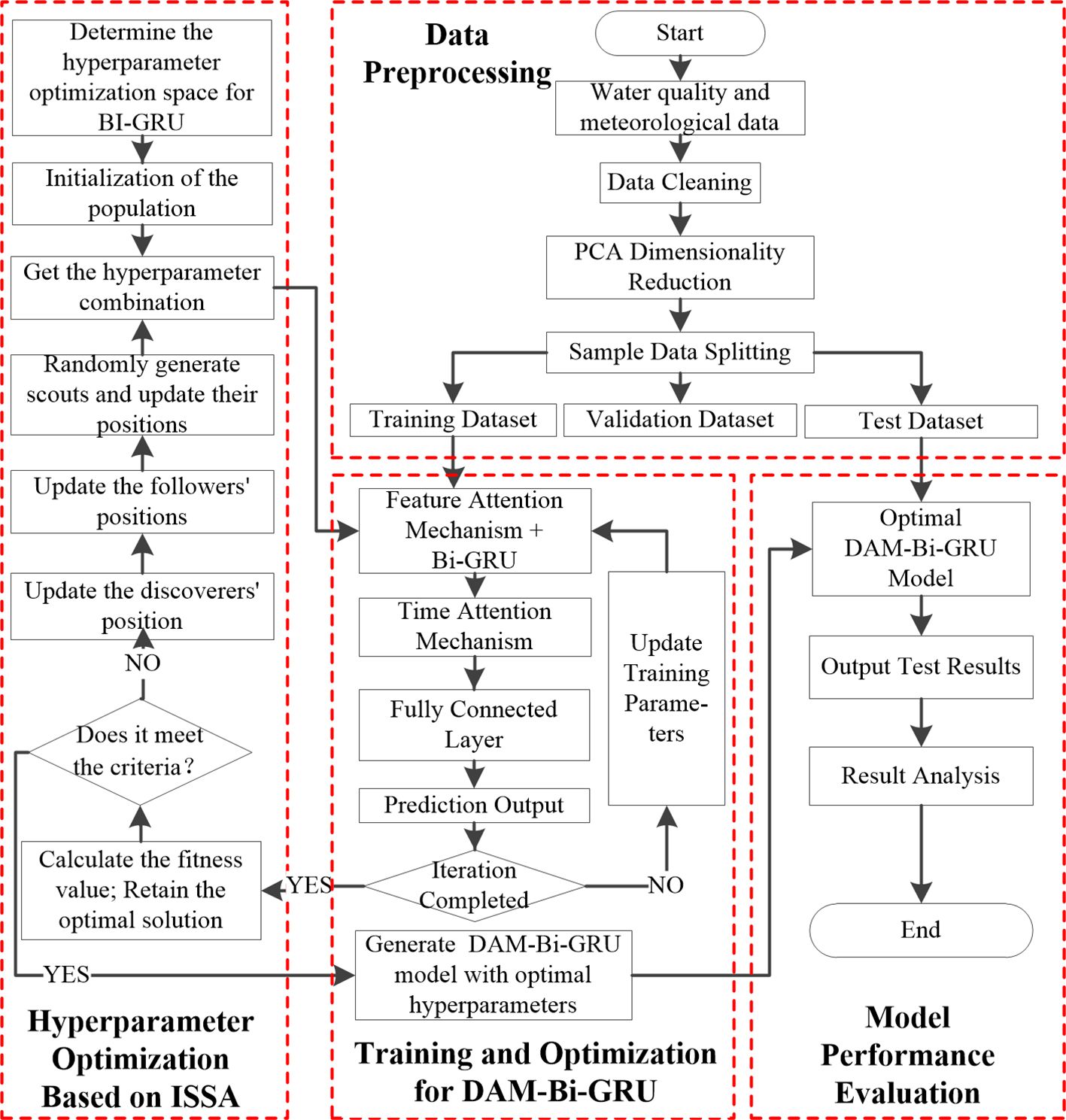
Figure 7. Flowchart of DO prediction algorithm PCA-ISSA-DAM-Bi-GRU.

3 Results

3.1 Data processing

To validate the performance of the proposed model in this article, data from the study area spanning 86 days from June 1st 2023 to August 25th 2023 were collected, with each data point recorded every 30 minutes, resulting in a total of 4,184 data sets for every given monitor point. The first 60 days’ data were used as the training set, the next 13 days’ data as the validation set, and the final 13 days’ data as the test set, following a 7:1.5:1.5 ratio. For any given time t, the model’s input comprised the aquaculture environmental parameters from the preceding 24 hours, and its output predicted the dissolved oxygen levels for the following 2 hours. This resulted in 2,832 training samples, 624 validation samples, and 624 test samples. Due to space limitations, a portion of the raw data collected on June 20th 2023 is presented in Table 1. Furthermore, taking monitor point A9 as an example, after removing outliers and filling in missing values through linear interpolation, statistical analysis was conducted on the data, as shown in Table 2. Subsequently, the PCA algorithm was applied to reduce the data’s dimensionality, eliminating redundant information and noise. Finally the processed data was input into the neural network model for feature extraction. The PCA of the aquaculture environmental parameters is presented in Table 3. As can be seen, the cumulative contribution rate of the first seven components reaches 86.27%, representing the majority of environmental information. Therefore, this study selected seven principal components, utilizing PCA to reduce the original 13-dimensional data to seven dimensions.

Table 1A

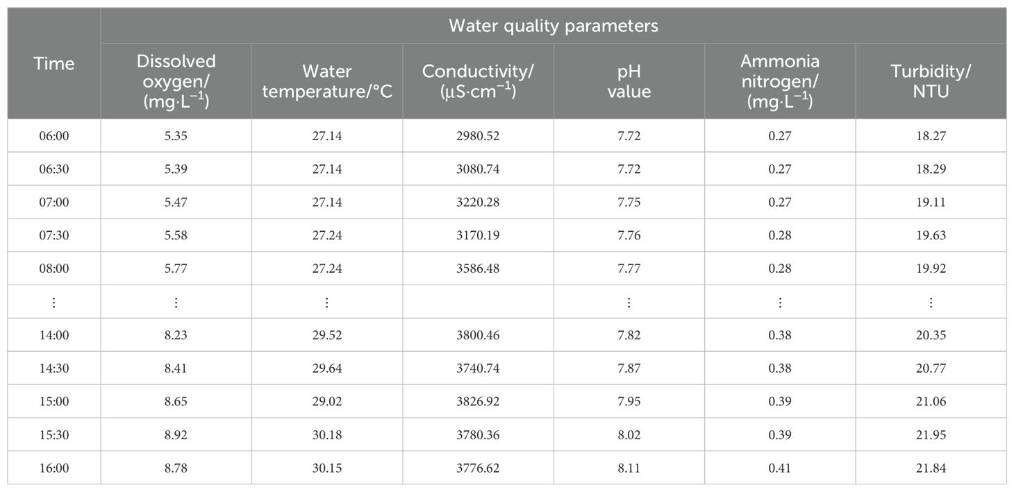
Table 1A. Water quality data collected by monitoring station A9 on June 20, 2023.

Table 1B

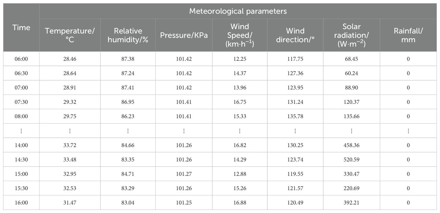
Table 1B. Meteorological parameter data collected by monitoring station A9 on June 20, 2023.

Table 2

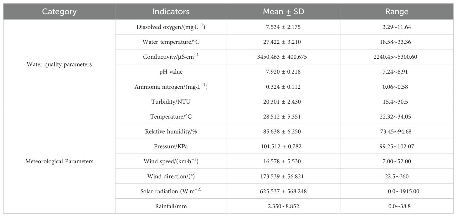
Table 2. Statistical results of data collected by monitoring station A9.

Table 3

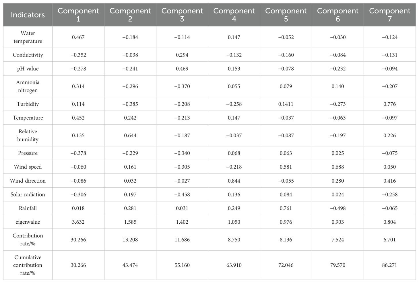
Table 3. Principal component coefficient matrix of aquaculture environment parameters.

3.2 Hyperparameter optimization and training of the model

The data, after being processed through outlier removal, linear interpolation for missing values, and principal component analysis, was input into the neural network model for hyperparameter optimization and training.

Step 1: Initialize the hyperparameters of the ISSA. The number of sparrows was set to 50, the maximum number of iterations T was 100, with the proportions of producers, followers, and scouts being 70%, 10%, and 20% respectively. The safety threshold was set to 0.6, and the search space was 5-dimensional. For the two-layer Bi-GRU, the optimization range for the number of hidden neurons was [8, 128], the optimization range for the maximum number of iterations was [10, 100], the optimization range for the batch size was [16, 128], and the optimization range for the learning rate was [0.001, 0.1].

Step 2: Train the DAM-Bi-GRU model using the hyperparameter combinations provided by ISSA. Each sparrow corresponds to a set of hyperparameter combinations. The model was trained using supervised learning, with the root mean square error (RMSE) function serving as the loss function. The mathematical definition of RMSE is as follows:

$\begin{array}{ll}\text{RMSE}=\sqrt{\frac{1}{N}{\displaystyle {\sum }_{i=1}^N{(y_i-{\widehat{y}}_i)}^2}}& (22)\end{array}$

where $y_i$ and ${\widehat{y}}_i$ represents the actual value and the predicted value by the model respectively, and N is the number of training samples in a batch. An end-to-end learning approach was adopted, where the neural network’s weights were continuously adjusted through forward propagation and backward propagation of gradients. The iteration stops once the preset number of iterations is reached or the training objective is achieved, completing the neural network training. Ultimately, each hyperparameter combination corresponds to a trained DAM-Bi-GRU model.

Step 3: Validate the DAM-Bi-GRU models trained in Step 2 using the pre-divided validation dataset. The validation result of each trained DAM-Bi-GRU model was measured by RMSE, and the fitness of the sparrow corresponding to the set of hyperparameter combinations for that model is also evaluated using the same RMSE value.

Step 4: Determining whether the model training has concluded based on the fitness value. If it has reaches the maximum number of the presented iterations of ISSA or the optimal fitness value of the sparrow population has met the training objective, end the training and output the DAM-Bi-GRU model with the optimal parameter combination. Otherwise, update the positions of producers, followers, and scouts based on the fitness values of the sparrow population, and generate new hyperparameter combinations. Repeat Steps 2 to 4 until the training is completed.

Following the above optimization and training steps, the final results of DAM-Bi-GRU hyperparameter optimization were obtained, with the hidden neuron counts for the two-layer Bi-GRU being 46 and 72 respectively; the maximum number of iterations being 86; the batch size being 66; and the learning rate being 0.004. Furthermore, the proposed ISSA was compared with the original SSA, PSO, and GA in terms of optimization performance. The convergence of the algorithms during the iterative optimization process is illustrated in Figure 8. It can be seen that the fitness value of ISSA converges to around 0.21 after approximately 35 iterations, while SSA converges to around 0.23 after about 45 iterations, PSO converges to around 0.26 after approximately 55 iterations, and GA converges to around 0.28 after approximately 70 iterations. This indicates that the optimization ability and convergence speed of ISSA are significantly higher than those of SSA, GA, and PSO. Additionally, the fluctuating downward trend of the fitness value of ISSA in Figure 8 suggests its ability to quickly escape local optima. In contrast, the other three optimization algorithms exhibit varying degrees of stagnation.

Figure 8

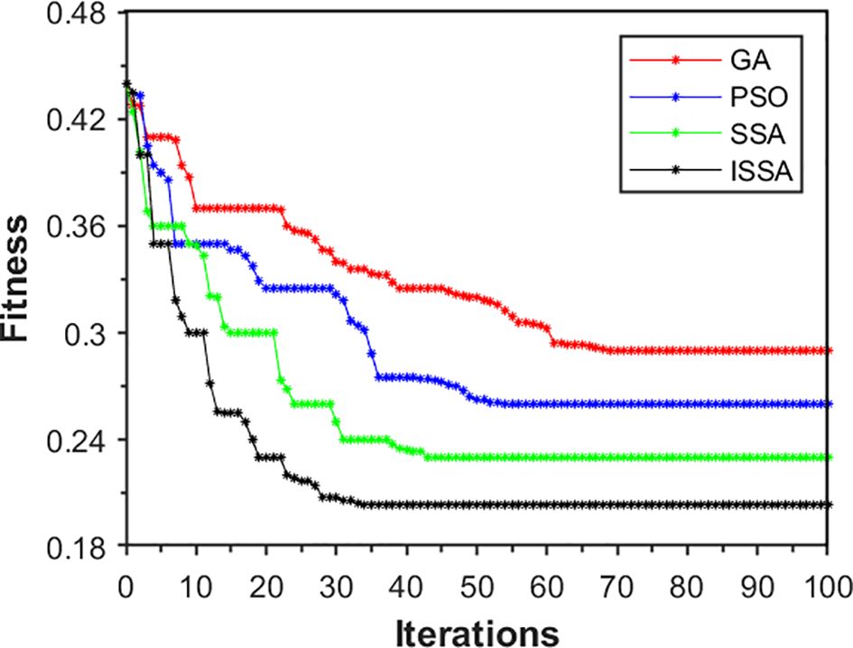
Figure 8. Iterative optimization and convergence curves for different optimization algorithm.

3.3 Testing and evaluation of the model

In this study, the root mean squared error (RMSE), mean absolute percentage error (MAPE), and Nash-Sutcliffe efficient (NSE) were adopted to evaluate the predictive performance of the model. The calculation formulas are as follows:

$\begin{array}{ll}\text{RMSE}=\sqrt{\frac{1}{N}{\displaystyle {\sum }_{i=1}^N{(y_i-{\widehat{y}}_i)}^2}}& (23)\end{array}$

$\begin{array}{ll}\text{MAPE}=\frac{1}{N}{\displaystyle {\sum }_{i=1}^N\left|\frac{y_i-{\widehat{y}}_i}{y_i}\right|}& (24)\end{array}$

$\begin{array}{ll}\text{NSE}=1-\frac{{\displaystyle {\sum }_{i=1}^N{(y_i-{\widehat{y}}_i)}^2}}{{\displaystyle {\sum }_{i=1}^N{(y_i-{\overline{y}}_i)}^2}}& (25)\end{array}$

where $y_i$ is the actual value, ${\overline{y}}_i$ is the mean of the actual values, ${\widehat{y}}_i$ is the predicted value by the model, and N is the number of data points in the data set used for evaluating the model’s performance. A lower RMSE indicates better predictive performance. MAPE measures the average magnitude of the percentage errors in a set of predictions, without considering their direction. A lower MAPE indicates better predictive accuracy. NSC ranges from negative infinity to 1, with 1 indicating a perfect match between observed and predicted values. Higher NSE values indicate better predictive performance. In summary, a lower RMSE and MAPE, and a higher NSC, all suggest better predictive performance of the model.

The 624 test data set samples were inputted one by one into the trained DAM-Bi-GRU model with the optimal combination of hyperparameters, the prediction results were obtained sequentially. The model’s performance parameters on the test set were calculated by Equations 23–25, namely RMSE, MAPE, and NSE which found to be 0.2136, 0.0232, and 0.9427, respectively. Additionally, Figures 9A–D sequentially present the comparison curves of predicted and actual values for the test samples, the prediction errors, the distribution of prediction errors, and the linear fitting between predicted and actual values. From Figure 9A, it can be observed that the proposed PCA-ISSA-DAM-Bi-GRU model is capable of capturing the changing trends of real dissolved oxygen data, sensitively identifying subtle fluctuations in the data, and maintaining a high prediction accuracy. Figures 9B–D demonstrate that there is a small discrepancy between the predicted and actual values.

Figure 9

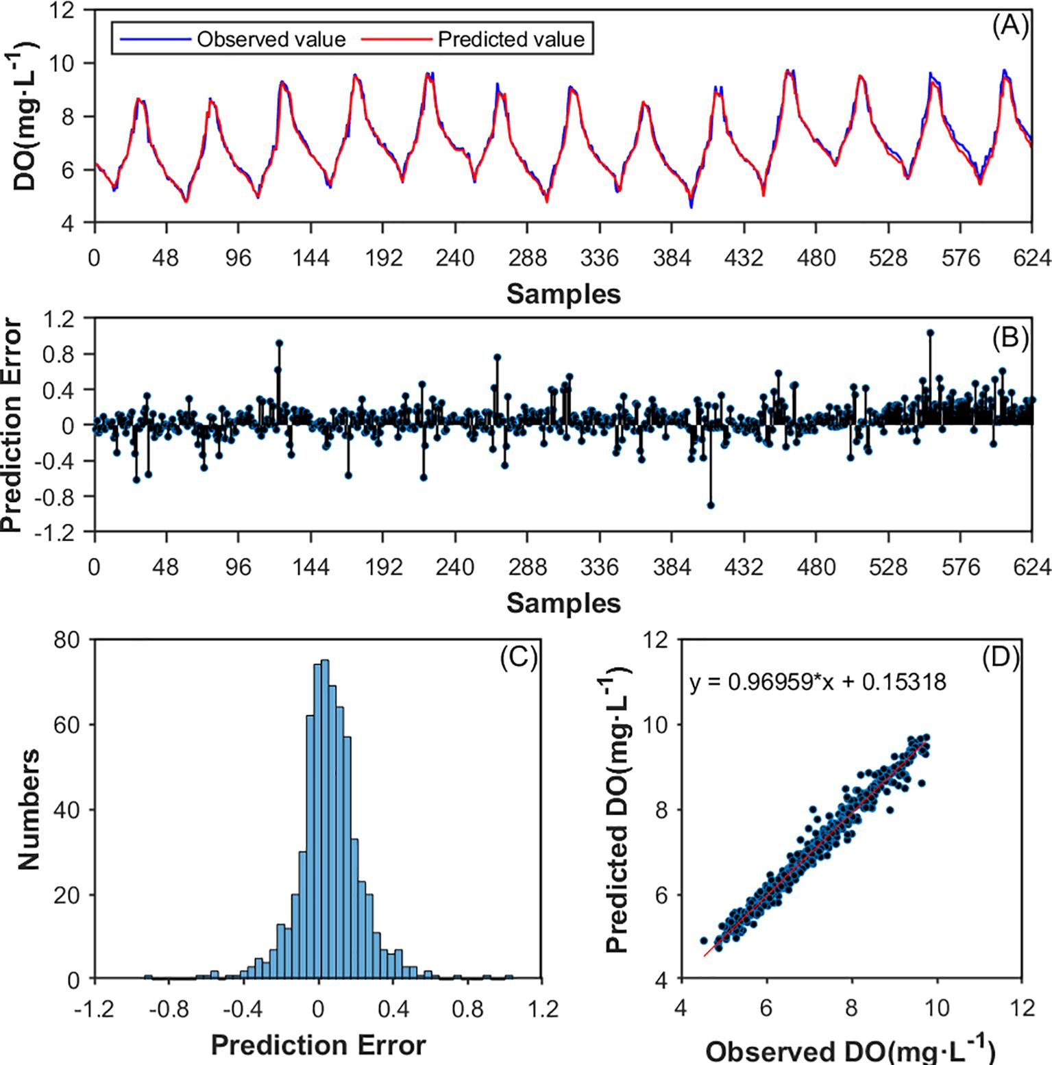
Figure 9. (A) DO prediction of the proposed model on the test data set. (B) Prediction error of the test data set; (C) Histogram of the prediction error distribution on the test data set; (D) Linear fitting between predicted and observed values.

3.4 Comparison and analysis of the models

To analyze and evaluate the competitiveness and superiority of the proposed model, this article designed ablation experiments and comparative experiments, selecting different models to compare their predictive performance.

3.4.1 Ablation experiments

The ablation experiments were conducted in two groups, A and B. The models in Group A do not incorporate the hyperparameter optimization module ISSA, with the baseline model being Bi-GRU. The models in Group B all include the ISSA, with the baseline model being ISSA-Bi-GRU. Each group include three models: one with PCA added alone to the baseline module, one with DAM added alone, and one with both PCA and DAM added simultaneously. For experiments in Group A, the random search method was used to determine the model’s hyperparameters with the number of random searches setted to be 100, which is equivalent to the maximum number of iterations for the ISSA module.

The prediction performance of each model on the test data set is shown in Table 4. In Group A, the prediction performance indicators RMSE, MAPE, and NSE of the baseline model Bi-GRU are 0.4077, 0.0527, and 0.8358, respectively. Compared with it, the PCA-Bi-GRU model shows a 9.22% decrease in RMSE, a 11.76% decrease in MAPE, and a 1.99% increase in NSE. The DAM-Bi-GRU model exhibits a 18.42% reduction in RMSE, a 28.27% reduction in MAPE, and a 5.56% increase in NSE. The PCA-DAM-Bi-GRU model, on the other hand, demonstrates a 24.63% decrease in RMSE, a 40.23% decrease in MAPE, and a 8.91% increase in NSE compared to the baseline. In Group B, the prediction performance indicators RMSE, MAPE, and NSE of the base model ISSA-Bi-GRU are 0.3424, 0.0392, and 0.8682, respectively. The PCA-ISSA-Bi-GRU model shows a 4.35% decrease in RMSE, a 8.16% decrease in MAPE, and a 3.44% increase in NSC compared to it. The ISSA-DAM-GRU model exhibits an 18.81% reduction in RMSE, a 17.6% reduction in MAPE, and a 6.73% increase in NSC. The PCA-ISSA-DAM-Bi-GRU model, however, demonstrates a 37.62% decrease in RMSE, a 40.82% decrease in MAPE, and an 8.85% increase in NSE compared to the base model. This indicates that both the DAM module and the PCA module can enhance the prediction performance of the models, with the DAM module showing a more significant improvement than PCA, and their fusion being even more effective. Figures 10A–C represent the three evaluation indicators (RMSE, MAPE, and NSE) for the models in Groups A and B, respectively. It can be observed that optimizing the hyperparameters of the Bi-GRU module through the ISSA module indeed enhances the prediction performance of the models.

Table 4

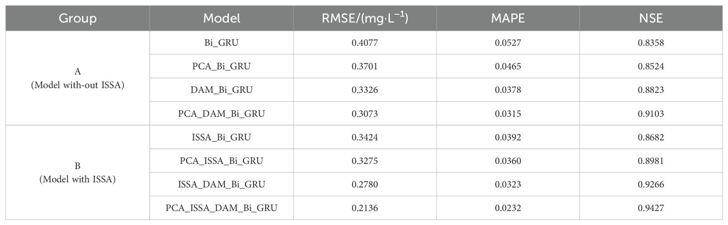
Table 4. Predictive performance of different models for the ablation experiments.

Figure 10

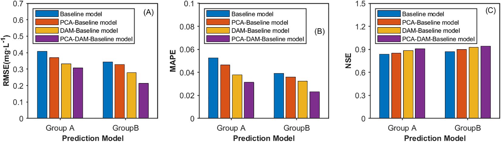
Figure 10. Prediction performance presented by (A) RMSE, (B) MARE and (C) NSE for various models in the ablation study. Group A do not incorporate attention mechanism and Group B incorporate attention Mechanism.

3.4.2 Comparative experiments

3.4.2.1 Comparison with baseline modules

To evaluate the superiority of PCA, ISSA, and Bi-GRU in enhancing prediction accuracy within the proposed model, the following comparative experiments were also conducted in this study: 1) Pearson correlation coefficient analysis was used to replace PCA, resulting in the comparative model P-ISSA-DAM-Bi-GRU; 2) ISSA was replaced with SSA, GA, and PSO, respectively, generating comparative models PCA-SSA-DAM-Bi-GRU, PCA-GA-DAM-Bi-GRU, and PCA-PSO-DAM-Bi-GRU; 3) Bi-GRU was replaced with Bi-LSTM, LSTM, and CNN, respectively, resulting in comparative models PCA-ISSA-DAM-Bi-LSTM, PCA-ISSA-DAM-LSTM, and PCA-ISSA-DAM-CNN. Eight comparative models were evaluated in total corresponding to serial numbers 1 to 8. The experimental results are presented in Table 5 and Figure 11, revealing the following: 1) The prediction performance metrics of the PCA-ISSA-DAM-Bi-GRU model are superior to those of P-ISSA-DAM-Bi-GRU, indicating that PCA outperforms the Pearson correlation coefficient analysis method in dimensionality reduction for data input in terms of dissolved oxygen prediction performance; 2) The prediction performance metrics of PCA-ISSA-DAM-Bi-GRU are superior to those of PCA-SSA-DAM-Bi-GRU, PCA-GA-DAM-Bi-GRU, and PCA-PSO-DAM-Bi-GRU, with the NSE value reaching 0.9807, demonstrating that compared to baseline approaches such as SSA, GA, and PSO, the optimization of Bi-GRU hyperparameters by ISSA results in better model fitting; 3) The prediction performance metrics of PCA-ISSA-DAM-Bi-GRU are slightly higher than those of PCA-ISSA-DAM-Bi-LSTM and significantly higher than those of PCA-ISSA-DAM-LSTM and PCA-ISSA-DAM-CNN, indicating that bidirectional neural networks enhance temporal feature extraction for contextually related time series prediction.

Table 5

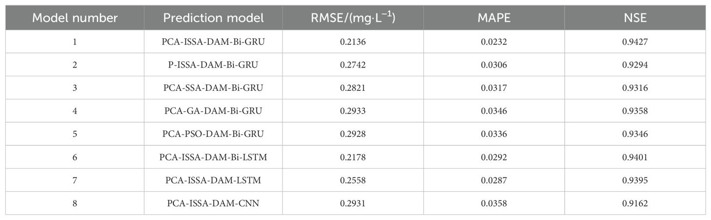
Table 5. Predictive performance of different models for the comparative experiments.

Figure 11

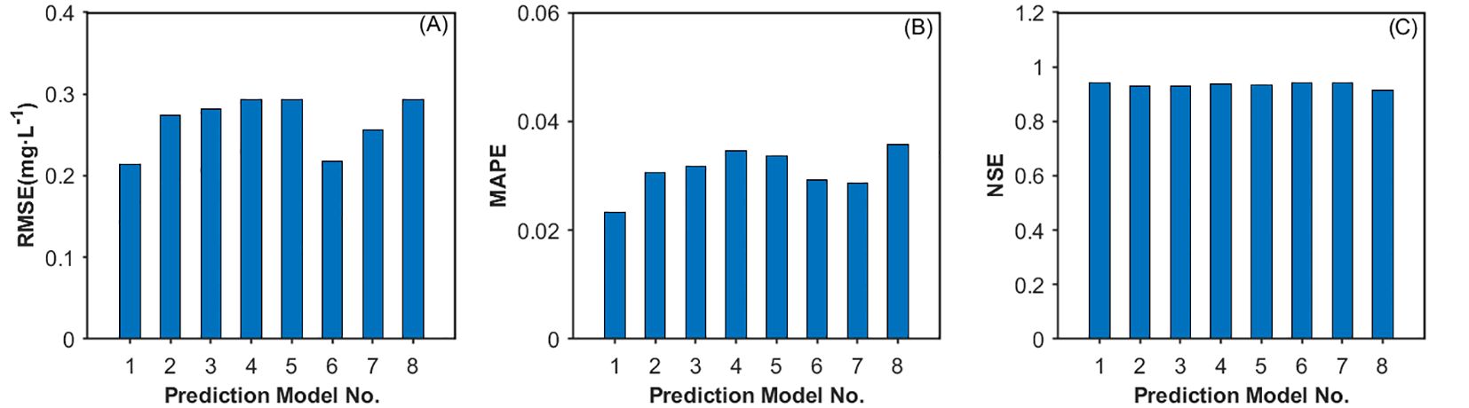
Figure 11. Prediction performance presented by (A) RMSE, (B) MARE and (C) NSE for various models in the comparative experiments.

3.4.2.2 Comparison with existing models

Furthermore, in order to test the overall predictive performance of the proposed hybrid model PCA-ISSA-DAM-Bi-GRU, this paper also selected dissolved oxygen prediction models proposed in the past three years, namely IPSO-LSTM (Cao et al., 2021b), IBAS-LSTM (Sun et al., 2021), CNN-LSTM (Tan et al., 2022) and IDA-GRU (Zhang et al., 2023) for comparison. The results in Table 6 show that the model proposed in this paper outperforms those 4 models, indicating the effectiveness and superiority of the individual modules and their fusion in enhancing the prediction accuracy of dissolved oxygen.

Table 6

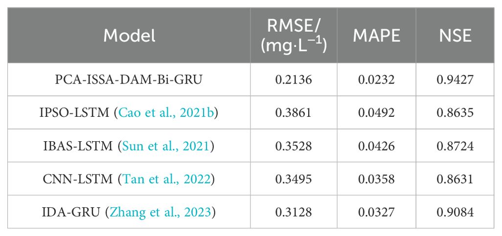
Table 6. Predictive performance of existing models.

3.5 Application of the model

To evaluate the practical effectiveness of the proposed model, the dissolved oxygen prediction for August 26, 2023, at the A9 monitoring station was selected as the experimental case. The prediction results and prediction error curves from the proposed PAC-ISSA-DAM-Bi-GRU model, along with the PCA-ISSA-Bi-GRU, PCA-DAM-Bi-GRU, IBAS-LSTM (Sun et al., 2021), and IDA-GRU (Zhang et al., 2023) models discussed in the previous section, are presented in Figure 12. The error value curves visually reflect the differences between the predicted curves and the actual curves, with smaller fluctuations and closer proximity to the zero-value line indicating better prediction performance. The analysis is as follows: 1) The prediction curve of the PCA-ISSA-DAM-Bi-GRU model proposed in this paper (Figures 12A, B) is closest to the actual observed values; 2) The prediction accuracy of PCA-ISSA-Bi-GRU without the dual attention mechanism (Figures 12E, F) and the IBAS-LSTM (Sun et al., 2021)model (Figures 12G, H) is significantly lower than that of the other three models, especially during the daytime. This maybe due to the factor that the dissolved oxygen is greatly affected by light intensity, and the introduced attention mechanism increases the weight of light intensity to improve the prediction accuracy; 3) The PCA-DAM-Bi-GRU model (Figures 12C, D), which do not incorporate hyperparameter optimization module ISSA, performs slightly better than IDA-GRU (Zhang et al., 2023) (Figures 12I, J), but both are significantly inferior to the PCA-ISSA-DAM-Bi-GRU model (Figures 12A, B) that incorporates ISSA for hyperparameter optimization.

Figure 12

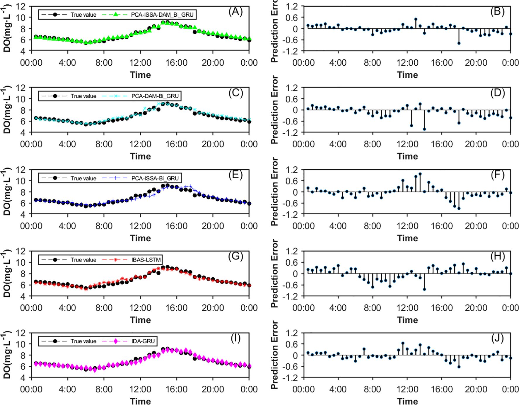
Figure 12. The prediction results and prediction error curves from five models on August 26, 2023. (A, B) PCA-ISSA-DAM-Bi-GRU model; (C, D) PCA-ISSA-Bi-GRU; (E, F) PCA-DAM-Bi-GRU; (G, H) IBAS-LSTM (Sun et al., 2021); (I, J) IDA-GRU (Zhang et al., 2023).

As can be seen from Figure 11, the daily dissolved oxygen reaches the peak at around 15:00 and reaches the valley value at around 06:00, which can reflect the health state of the water environment to a large extent. Figure 13 presents the predicted dissolved oxygen distribution at various depths and monitoring stations at 06:00 and 15:00 on August 26, 2023, using the proposed PCA-ISSA-DAM-Bi-GRU model. The analysis of this distribution provides valuable insights into the health status of the aquatic environment. The key observations are: 1) Vertical dissolved oxygen gradient: compared Figures 13A–D, it could be concluded that within the same vertical profile, the dissolved oxygen levels at 1.6 meters depth are consistently lower than those at 0.8 meters, with this difference being more pronounced during the day compared to night. This vertical gradient is a common phenomenon in aquatic systems, where oxygen solubility decreases with depth due to factors such as temperature and pressure. 2) Spatial variations during daytime: it could be seen from Figure 13A that during the day, the dissolved oxygen concentration in regions A1, A2, and A4 is higher than in A3 and A7. This can be attributed to various factors, including wind direction, water temperature, and the photosynthetic activity of aquatic plants (e.g., phytoplankton). Favorable wind conditions can enhance mixing and oxygenation, while increased photosynthetic activity during daylight hours releases oxygen into the water. 3) Spatial variations during nighttime: it could be seen from Figure 13C that The distribution of dissolved oxygen at night is influenced by different factors, such as the aggregation patterns of fish schools, wind direction, and the location of feeding devices. Notably, the dissolved oxygen levels in regions A1 and A9 are higher, while those in A7 and A8 are lower. This can be explained by the possible concentration of fish schools or the efficiency of oxygen replenishment mechanisms in these areas. Additionally, the reduced photosynthetic activity at night leads to a general decrease in dissolved oxygen levels across all regions.

Figure 13

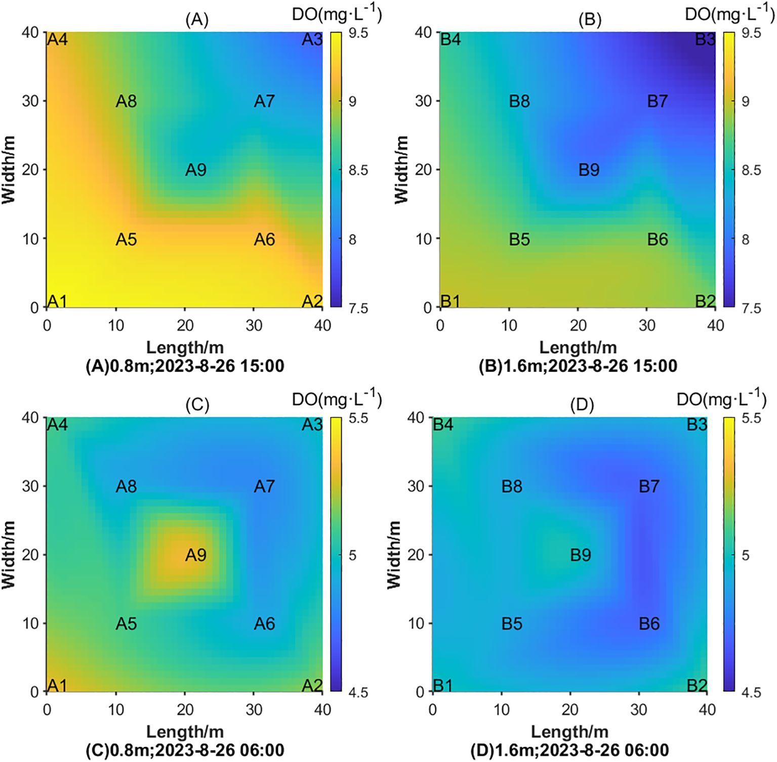
Figure 13. Dissolved oxygen distribution on different time at different water layers on August 26th 2023. (A) Dissolved oxygen distribution at a depth of 0.8 meters on 15:00; (B) Dissolved oxygen distribution at a depth of 1.6 meters on 15:00; (C) Dissolved oxygen distribution at a depth of 0.8 meters on 06:00; (D) Dissolved oxygen distribution at a depth of 1.6 meters on 06:00.

The observed diurnal and spatial variations in dissolved oxygen concentrations highlight the complexity of aquatic ecosystems and the importance of accurate monitoring and prediction. The PCA-ISSA-DAM-Bi-GRU model, by capturing these dynamic changes, provides a powerful tool for assessing the health of aquaculture systems and informing management decisions aimed at optimizing conditions for fish growth and welfare.

4 Discussion

4.1 Optimization mechanism of ISSA

As can be observed from Figure 8, the proposed ISSA in this study exhibits superior capability in optimizing model hyperparameters and convergence speed compared to the original SSA, GA, and PSO. Table 5 further indicates that the DO prediction performance of Bi-GRU optimized by ISSA is superior to that optimized by SSA, GA, and PSO. The optimization capability and convergence speed of SSA are primarily influenced by factors such as population diversity, global search performance, and local search ability. ISSA employs a multi-strategy fusion approach for improvement, which not only enhances the diversity and quality of the initial population but also fully utilizes information exchange among sparrow individuals to achieve a balance between local exploitation and global search in the algorithm. Additionally, it improves the algorithm’s ability to escape from local extrema. Firstly, the introduction of Gauss chaotic sequence into the population initialization process ensured a uniform distribution of the initial population, thereby enhancing population diversity and the global search performance of the model. Secondly, the improvement of the position update strategy for discoverers by drawing inspiration from the Salp Swarm Algorithm allowing the discoverers to not necessarily decrease in every dimension during the early iterations, enhancing the search range and global search capability of the population while also maintaining the convergence speed and local search ability during the later iterations of the algorithm. Furthermore, the improvement of the position update process for followers by adopting the random following strategy from the Chicken Swarm Optimization (CSO) algorithm, where hens converge towards roosters with a certain probability. This ensures both convergence and population diversity, balancing local exploitation and global search. Lastly, the introduction of the Cauchy-Gaussian mutation strategy maintains population diversity and resistance to stagnation, preventing premature convergence of the algorithm.

4.2 Optimization effects of each module in the proposed PAC-ISSA-DAM-Bi-GRU

Based on ablation and comparison experiments, the analysis of the optimization effects of each module in the PCA-ISSA-DAM-Bi-GRU model on DO prediction is as follows: 1) ISSA can optimize the hyperparameters of the neural network model, thereby enhancing its prediction performance for the factor that hyperparameters control the structure, topology, and training process of the network, directly impacting the model’s fitting degree, generalization ability, and stability during training. 2) Dimensionality reduction of data using PCA can improve model performance, and the effect is superior to that of the Pearson correlation coefficient analysis method. This is because the Pearson correlation coefficient analysis method only selects factors with high correlation coefficients with dissolved oxygen as inputs, completely ignoring factors weakly correlated with dissolved oxygen. In contrast, the PCA analysis method used in this study can capture 86.27% of water quality and meteorological information with only 7 dimensions of data. While reducing the dimensionality, it ensures that the input information is more complete and comprehensive, facilitating subsequent feature extraction. 3) The DAM module introduces a dual attention mechanism combining feature and temporal attention. The feature attention mechanism adaptively assigns weights to different environmental factors at each time point, while the temporal attention mechanism dynamically adjusts the weights of different time steps on the current DO concentration. This enables the neural network to better capture critical information in time series data. 4) The prediction performance of Bi-GRU is significantly higher than that of LSTM and CNN. This is because the dissolved oxygen concentration at a particular moment is correlated with environmental factors both before and after it. Bi-GRU can simultaneously explore the sequential and inverse correlations in time series, comprehensively extracting temporal features.

4.3 Competitiveness and superiority compared to existing models

4.3.1 Comparison with IPSO-LSTM and IBAS-LSTM

Both the IPSO-LSTM (Cao et al., 2021b) and IBAS-LSTM (Sun et al., 2021) models employed modified optimization algorithms, IPSO and IBAS, respectively, to optimize the hyperparameters of LSTM networks. In contrast to the PCA-ISSA-DAM-Bi-GRU model proposed in this paper, neither of these models performed PCA dimensionality reduction nor incorporates the feature and temporal attention mechanism DAM. Firstly, an ISSA-Bi-GRU model was constructed, and experiments revealed that its prediction performance was slightly higher than that of IPSO-LSTM (Cao et al., 2021b) and IBAS-LSTM (Sun et al., 2021), as shown in Table 7. This demonstrates the superiority of the ISSA and Bi-GRU modules proposed in this paper. Therefore, the optimization capabilities and convergence speeds of ISSA, IPSO, and IBAS were compared in this paper. As shown in Figure 14 and significantly higher than those of IPSO. This demonstrates that the ISSA, with its enhanced search mechanisms and adaptive parameter adjustments, exhibits superior performance in finding optimal solutions and converging towards them efficiently, compared to the other two algorithms. Furthermore, PCA-IPSO-DAM-LSTM and PCA-IBAS-DAM-LSTM were constructed based on IPSO-LSTM (Cao et al., 2021b) and IBAS-LSTM (Sun et al., 2021), respectively. Significant improvements in prediction performance were observed as shown in Table 7, thoroughly validating the effectiveness of PCA and DAM proposed in this paper in enhancing the predictive capabilities of the models.

Table 7

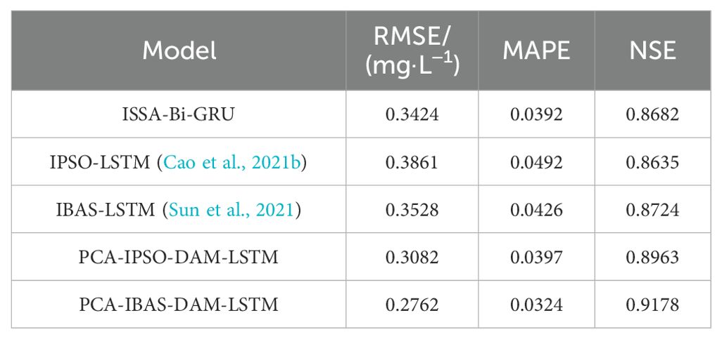
Table 7. Predictive performance of various models.

Figure 14

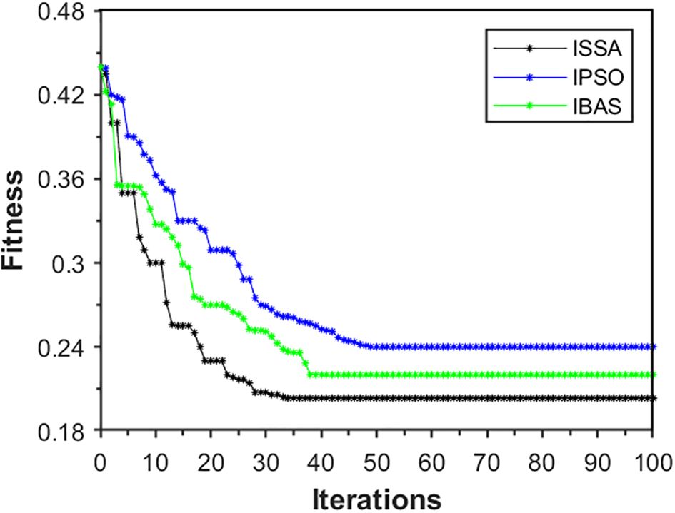
Figure 14. Iterative optimization and convergence curve for different optimization algorithm.

4.3.2 Comparison with CNN-LSTM

CNN-LSTM (Tan et al., 2022) employed CNN to extract local features from the data before feeding them into the LSTM network. Compared to the PCA-ISSA-DAM-Bi-GRU model proposed in this paper, CNN-LSTM functionally lacks the integration of the feature and temporal attention mechanism DAM, as well as the utilization of ISSA for optimizing the hyperparameters of the neural network. Firstly, PCA-Bi-GRU model was constructed for comparative experiments, with hyperparameter optimized through random search. Experimental results in Table 8 indicated that its predictive performance was slightly inferior to CNN-LSTM (Tan et al., 2022), suggesting that the combination of CNN and LSTM indeed enhances the feature extraction capability of the data. Furthermore, CNN-ISSA-DAM-LSTM model was built upon CNN-LSTM (Tan et al., 2022). Experiments revealed significant improvement in predictive performance as shown in Table 8, which reaffirms the effectiveness of the ISSA and DAM proposed in this paper in enhancing the predictive functionality of the model.

Table 8

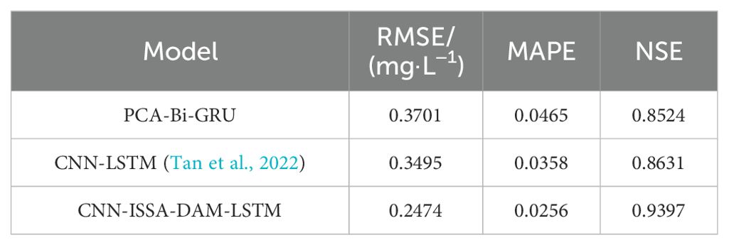
Table 8. Predictive performance of existing models.

4.3.3 Comparison with IDA-GRU

IDA-GRU (Zhang et al., 2023) employed a dual attention mechanism similar to this paper to optimize the hyperparameters of GRU, incorporating both feature and temporal attention at the input ends of the GRU encoder and decoder. However, its optimization effect is inferior to the model presented in this paper. Firstly, IDA-GRU (Zhang et al., 2023) utilized the Pearson correlation coefficient method to select environmental factors with high correlation coefficients with DO as input variables, whereas this paper adopts PCA, preserving approximately 86.27% of the information from all environmental factors. Secondly, IDA-GRU (Zhang et al., 2023) did not employ an intelligent optimization algorithm for hyperparameter tuning. In the comparison experiment, random search method was used to determine its hyperparameters, but its predictive performance still lags behind the model in this paper. This underscores the effectiveness of the ISSA proposed in this paper in enhancing the predictive performance of the model.

4.4 Practical application significance, limitations, and future research prospects of the model

This model utilized historical data from the past 24 hours to make real-time predictions of dissolved oxygen concentration 2 hours ahead, combined with LoRa+5G-based sensor deployment, enabling simultaneous prediction of dissolved oxygen concentrations at multiple points, thereby effectively forecasting the dissolved oxygen distribution in aquaculture areas. The engineering application analysis of the model reveals that it achieves good prediction results, effectively guiding water quality early warning and regulation, reducing aquaculture risks in marine ranching, and enhancing aquaculture efficiency. However, this study has limitations in spatial dimension prediction. The spatial distribution of dissolved oxygen was achieved through joint multi-point prediction, and the prediction accuracy of dissolved oxygen between points is related to the density of sensor deployment. Moreover, due to the limited availability of observed data, this study does not discuss the prediction performance of the model under different weather conditions. In future research, we will add more monitoring points in depth and attempt to employ a 3D convolutional neural network (3D-CNN) to capture the spatiotemporal characteristics of the data, providing more accurate prediction results. Additionally, we will further extend the experimental period to accumulate more data, which will be clustered according to weather conditions before predictive modeling for different categories, thereby enhancing the applicability and accuracy of the model.

5 Conclusion

To enhance the accuracy, generalization, and robustness of the dissolved oxygen prediction model in aquaculture water, this paper constructed a data-driven dissolved oxygen prediction model that integrates principal component analysis (PCA), dual attention mechanism (DAM), and bi-directional gated recurrent unit (Bi-GRU) neural network. Furthermore, an improved sparrow search algorithm with multi-strategy fusion (ISSA) is introduced for hyperparameter optimization. The main conclusions are as follows:

1. By applying PCA, the 13-dimensional input is reduced to 7 dimensions, eliminating redundancy and correlation among variables. This enhances the feature representation power of the input data for the prediction model and reduces its complexity. The fusion of DAM and Bi-GRU strengthens the feature extraction capability of the prediction model. The introduction of the feature attention mechanism in the encoder stage adaptively assigns weights to different environmental factors at each time step, while the time attention mechanism in the decoder stage dynamically adjusts the weights of the influence of different time steps on the current dissolved oxygen concentration. This enables the model to better capture the key information in the time series data. Combined with Bi-GRU, it simultaneously mines the sequential and inverse sequential correlations in the time series, comprehensively extracting temporal features.

2. The hyperparameters of the Bi-GRU model are searched and optimized using ISSA to enhance the model’s optimal learning capability. The Gauss chaotic sequence is introduced into the population initialization, and the updating strategy of the discoverer’s position is improved by referencing the salp swarm algorithm. Meanwhile, the updating strategy of the follower’s position is optimized by drawing inspiration from the chicken swarm algorithm, and the Cauchy-Gaussian mutation strategy is incorporated to enhance the convergence performance of the SSA algorithm, balancing its global search and local exploitation capabilities.

3. The root mean square error (RMSE), mean absolute percentage error (MAPE), and Nash-Sutcliffe efficiency (NSE) of the proposed PCA-ISSA-DAM-Bi-GRU model for predicting dissolved oxygen are 0.2136, 0.0232, and 0.9427, respectively. The ablation study demonstrates that each component of the hybrid model contributes to enhancing the predictive performance of the model. By comparing the results with traditional baseline approaches, it is evident that each module in the hybrid model provides a more significant optimization effect on prediction accuracy.

4. By combining the proposed model with wireless sensor deployment, it can effectively predict the spatio-temporal distribution characteristics of dissolved oxygen in aquaculture water, enabling dynamic monitoring of water quality in marine ranching and intelligent analysis of the aquaculture environment, thereby facilitating the construction of modern marine ranching.

In summary, the model proposed in this paper, combined with wireless sensor deployment, can effectively predict the spatio-temporal distribution characteristics of dissolved oxygen in aquaculture water bodies. This enables dynamic monitoring of water quality in marine ranching and intelligent analysis of the aquaculture environment, thereby contributing to the modernization of marine ranching construction. The model provides a powerful tool for managing and optimizing aquaculture operations, ensuring sustainable development and improved productivity in marine ranching systems.

Data availability statement

The raw data supporting the conclusions of this article will be made available by the authors, without undue reservation.

Author contributions

WL: Conceptualization, Formal analysis, Funding acquisition, Investigation, Methodology, Resources, Software, Validation, Visualization, Writing – original draft, Writing – review & editing. JW: Conceptualization, Methodology, Writing – review & editing. ZL: Software, Visualization, Writing – review & editing. QL: Data curation, Visualization, Writing – review & editing.

Funding

The author(s) declare that financial support was received for the research, authorship, and/or publication of this article. This work was supported by the Key R&D Program of Shaanxi Province (2023-ZDLGY-15); General Project of National Natural Science Foundation of China (51979045); New Generation Information Technology Special Project in Key Fields of Ordinary Universities in Guangdong Province (2020ZDZX3008); Key Special Project in the Field of Artificial Intelligence in Guangdong Province (2019KZDZX1046); University level doctoral initiation project (060302112309); Guangdong Youth Fund Project (2023A15151110770); Zhanjiang Marine Youth Talent Innovation Project (2023E0010).

Conflict of interest

The authors declare that the research was conducted in the absence of any commercial or financial relationships that could be construed as a potential conflict of interest.

Publisher’s note

All claims expressed in this article are solely those of the authors and do not necessarily represent those of their affiliated organizations, or those of the publisher, the editors and the reviewers. Any product that may be evaluated in this article, or claim that may be made by its manufacturer, is not guaranteed or endorsed by the publisher.

References

Abdel-Tawwab M., Monier M. N., Hoseinifar S. H., Faggio C. (2019). Fish response to hypoxia stress: growth, physiological, and immunological biomarkers. Fish Physiol. Biochem. 45, 997. doi: 10.1007/s10695-019-00614-9

Crossref Full Text | Google Scholar

Arora S., Keshari A. K. (2021). Dissolved oxygen modelling of the Yamuna river using different ANFIS models. Water Sci. Technol. 84, 3359–3371. doi: 10.2166/wst.2021.466

Crossref Full Text | Google Scholar

Cao S., Zhou L., Zhang Z. (2021a). Prediction of dissolved oxygen content in aquaculture based on clustering and improved ELM. IEEE Access PP, 1–1. doi: 10.1109/access.2021.3064029

Crossref Full Text | Google Scholar

Cao S., Zhou L., Zhang Z. (2021b). Prediction model of dissolved oxygen in aquaculture based on improved long short-term memory neural network. Trans. Chin. Soc. Agric. Eng. (Transactions CSAE) 37, 235–242. doi: 10.11975/j.issn.1002-6819.2021.14.027

Crossref Full Text | Google Scholar

Chen H., Yang J., Fu X., Zheng Q., Song X., Fu Z., et al. (2022). Water quality prediction based on LSTM and attention mechanism: A case study of the Burnett River, Australia. Sustainability 14, 13231. doi: 10.3390/su142013231

Crossref Full Text | Google Scholar

Choi H., Suh S.-I., Kim S.-H., Han E. J., Ki S. J. (2021). Assessing the performance of deep learning algorithms for short-term surface water quality prediction. Sustainability 13, 10690. doi: 10.3390/su131910690

Crossref Full Text | Google Scholar

Cuenco M. L., Stickney R. R., Grant W. E. (1985). Fish bioenergetics and growth in aquaculture ponds: ii. effects of interactions among, size, temperature, dissolved oxygen, unionized ammonia and food on growth of individual fish. Ecol. Modelling 27, 191–206. doi: 10.1016/0304-3800(85)90002-X

Crossref Full Text | Google Scholar

Guo Y., Chen S., Li X., Cunha M., Jayavelu S., Cammarano D., et al. (2022). Machine learning-based approaches for predicting SPAD values of maize using multi-spectral images. Remote Sens. 14, 1337. doi: 10.3390/rs14061337

Crossref Full Text | Google Scholar

Guo Y., Xiao Y., Hao F., Zhang X., Chen J., de Beurs K., et al. (2023). Comparison of different machine learning algorithms for predicting maize grain yield using UAV-based hyperspectral images. Int. J. Appl. Earth Observation Geoinf. 124, 103528. doi: 10.1016/j.jag.2023.103528

Crossref Full Text | Google Scholar

Huan J., Li M., Xu X., Zhang H., Yang B., Jiang J., et al. (2022). Multi-step prediction of dissolved oxygen in rivers based on random forest missing value imputation and attention mechanism coupled with recurrent neural network. Water Supply 22, 5480–5493. doi: 10.2166/ws.2022.154

Crossref Full Text | Google Scholar

Jiange J., Liqin Z., Senjun H. (2023). Water quality prediction based on IGRA-ISSA-LSTM model. Water Air Soil pollut. 234, 172. doi: 10.1007/s11270-023-06117-x

Crossref Full Text | Google Scholar

Jiang X., Dong S., Liu R., Huang M., Dong K., Ge J., et al. (2021). Effects of temperature, dissolved oxygen, and their interaction on the growth performance and condition of rainbow trout (Oncorhynchus mykiss). J. Of Thermal Biol. 98, 102928. doi: 10.1016/j.jtherbio.2021.102928

Crossref Full Text | Google Scholar

Kuang L., Shi P., Hua C., Chen B., Zhu H. (2020). An enhanced extreme learning machine for dissolved oxygen prediction in wireless sensor networks. IEEE Access 8, 198730–198739. doi: 10.1109/ACCESS.2020.3033455

Crossref Full Text | Google Scholar

Li W., Wu H., Zhu N., Jiang Y., Tan J., Guo Y. (2021). Prediction of dissolved oxygen in a fishery pond based on gated recurrent unit (GRU). Inf. Process. Agric. 8, 185–193. doi: 10.1016/j.inpa.2020.02.002

Crossref Full Text | Google Scholar

Li Y., Li X., Xu C., Tang X. (2023). Dissolved oxygen prediction model for the Yangtze River estuary basin using IPSO-LSSVM. Water 15, 2206. doi: 10.3390/w15122206

Crossref Full Text | Google Scholar

Lipizer M., Partescano E., Rabitti A., Giorgetti A., Crise A. (2014). Qualified temperature, salinity and dissolved oxygen climatologies in a changing Adriatic sea. Ocean Sci. Discussions 11, 331–390. doi: 10.5194/os-10-771-2014

Crossref Full Text | Google Scholar

Liu P., Wang J., Sangaiah A., Xie Y., Yin X. (2019). Analysis and prediction of water quality using LSTM deep neural networks in ioT environment. Sustainability 11, 2058. doi: 10.3390/su11072058

Crossref Full Text | Google Scholar

Liu Y., Zhang Q., Song L., Chen Y. (2019). Attention-based recurrent neural networks for accurate short-term and long-term dissolved oxygen prediction. Comput. Electron. Agriculture 165, 104964. doi: 10.1016/j.compag.2019.104964

Crossref Full Text | Google Scholar

Mirjalili S., Gandomi A. H., Mirjalili S. Z., Saremi S., Faris H., Mirjalili S. M. (2017). Salp swarm algorithm: a bio-inspired optimizer for engineering design problems. Adv. Eng. Software 114, 163–191. doi: 10.1016/j.advengsoft.2017.07.002

Crossref Full Text | Google Scholar

Neilan R. M., Rose K. (2014). Simulating the effects of fluctuating dissolved oxygen on growth, reproduction, and survival of fish and shrimp. J. Theor. Biol. 343, 54–68. doi: 10.1016/j.jtbi.2013.11.004

Crossref Full Text | Google Scholar

Osamy W., El-Sawy A. A., Salim A. (2020). CSOCA: Chickenswarm optimization based clustering algorithm forwireless sensor networks. IEEE Access 8, 60676–60688. doi: 10.1109/ACCESS.2020.2983483

Crossref Full Text | Google Scholar

Sharad T., Richa B., Gagandeep K. (2018). Performance evaluation of two ANFIS models for predicting water quality index of river Satluj (India). Adv. Civil Eng. 2018, 1–10. doi: 10.1155/2018/8971079

Crossref Full Text | Google Scholar

Sun L., Wu Y., Sun X., Zhang S. (2021). Dissolved oxygen prediction model in ponds based on improved beetle antennae search and LSTM network. Trans. Chin. Soc. Agric. Machinery 52, 252–260. doi: 10.6041/j.issn.1000-1298.2021.S0.031

Crossref Full Text | Google Scholar

Tan W., Zhang J., Wu J., Lan H., Liu X., Xiao K., et al. (2022). Application of CNN and long short-term memory network in water quality predicting. Intell. Autom. Soft Comput. 34, 1943–1958. doi: 10.32604/iasc.2022.029660

Crossref Full Text | Google Scholar

Than N. H., Ly C. D., Van Tat P. (2021). The performance of classification and forecasting Dong Nai River water quality for sustainable water resources management using neural network techniques. J. Hydrol. 596, 126099. doi: 10.1016/j.jhydrol.2021.126099

Crossref Full Text | Google Scholar

Wang W. C., Xu L., Chau K. W., Xu D. M. (2020). Yin-Yang firefly algorithm based on dimensionally Cauchy mutation. Expert Syst. With Applications 150, 113216. doi: 10.1016/j.eswa.2020.113216

Crossref Full Text | Google Scholar

Wang J., Xie Z., Mo C. (2023). Research progress in accurate prediction of aquaculture water quality by neural network. J. Fish China. 47(8), 089502. doi: 10.11964/jfc.20220913689

Crossref Full Text | Google Scholar

Wu J., Li Z., Zhu L., Li G., Niu B., Peng F. (2018). Optimized BP neural network for Dissolved Oxygen prediction. IFAC-PapersOnLine 51, 596–601. doi: 10.1016/j.ifacol.2018.08.132

Crossref Full Text | Google Scholar

Xue J., Shen B. (2020). A novel swarm intelligence optimization approach: Sparrow search algorithm. Syst. Sci. Control Engineering 8, 22–34. doi: 10.1080/21642583.2019.1708830

Crossref Full Text | Google Scholar

Yang H., Liu S. (2022). Water quality prediction in sea cucumber farming based on a GRU neural network optimized by an improved whale optimization algorithm. PeerJ Comput. Sci. 8, e1000. doi: 10.7717/peerj-cs.1000

Crossref Full Text | Google Scholar

Zhang Y.-F., Fitch P., Thorburn P. J. (2020). Predicting the trend of dissolved oxygen based on the kPCA-RNN model. Water 12, 585. doi: 10.3390/w12020585

Crossref Full Text | Google Scholar

Zhang Z., Jia X., Zhang Z., Cao S. (2023). Spatiotemporal prediction model of dissolved oxygen in aquaculture intergrating IDA-GRU and IIDW. Trans. Chin. Soc. Agric. Engineering 39, 161–171. doi: 10.11975/j.issn.1002-6819.202307067

Crossref Full Text | Google Scholar

Zhu C., Liu X., Ding W. (2017). “Prediction model of dissolved oxygen based on FOA-LSSVR,” in IEEE 2017 36th Chinese Control Conference (CCC), Dalian, China, July 26-28, 2017. IEEE, 9819–9823. doi: 10.23919/ChiCC.2017.8028922

Crossref Full Text | Google Scholar

Zhu N., Xia Q., Tan J., Jiang Y., Xu G., Chu D., et al. (2019). Model-based prediction of dissolved oxygen content in fish production. Trans. ASABE 62, 1417–1425. doi: 10.13031/trans.13263

Crossref Full Text | Google Scholar