Optimizing data-driven arctic marine forecasting: a comparative analysis of MariNet, FourCastNet, and PhyDNet

Introduction: Marine forecasts play a crucial role in ensuring safe navigation, efficient offshore operations, coastal management, and research, particularly in regions with challenging conditions like the Arctic Ocean. These forecasts necessitate precise predictions of ocean currents, wind-driven waves, and various other oceanic parameters. Although physics-based numerical models are highly accurate, they come with significant computational requirements. Therefore, data-driven approaches, which are less computationally intensive, may present a more effective solution for predicting sea conditions.

Methods: This study introduces a detailed analysis and comparison of three data-driven models: the newly developed convLSTM-based MariNet, FourCastNet, and PhydNet, a physics-informed model designed for video prediction. Through the utilization of metrics such as RMSE, Bias, and Correlation, we illustrate the areas in which our model outperforms well-known prediction models.

Results: Our model demonstrates enhanced accuracy in forecasting ocean dynamics when compared to FourCastNet and PhyDNet. Additionally, our findings reveal that our model demands significantly less training data and computational resources, ultimately resulting in lower carbon emissions.

Discussion: These findings indicate the potential for further exploration of data-driven models as a supplement to physics-based models in operational marine forecasting, as they have the capability to improve prediction accuracy and efficiency, thereby facilitating more responsive and cost-effective forecasting systems.

1 Introduction

Machine Learning is the process of making computer systems learn without explicit instructions by analyzing and drawing inferences from data patterns using algorithms and statistical models. One of the major limitations of Artificial Intelligence and Machine Learning has always been computational power, which has been a cause of concern for researchers. CPUs were not as powerful and efficient a few decades ago when it came to running large computations for machine learning. Hardware manufacturers have worked hard to create a processing unit capable of performing any AI operation.

Though CPUs are no longer viable sources of computational power, they were the pioneers. Today, those CPUs are rightfully replaced by GPUs and AI accelerators, specifically designed for large computing. The main features considered while purchasing an AI accelerator are cost, energy consumption, and processing speed.

The study of ocean circulation is crucial for many reasons, including the climate research, determining marine life distribution, shaping human activity, and more. Accurate prediction of currents can help forecast weather, estimate energy transfer rates in the ocean, predict the spread of oil spills and drift of the sea ice and icebergs. Sediment transport is another important correlated aspect correlated with the water circulation, affecting marine economic activities such as fishing, transport, logistics, and tourism. Therefore, in the seas, especially in the high latitudes, the prediction of currents is crucial for port, pipeline, and logistics development, as well as for the analysis of sea ice drift for safe logistics. In this context, the development of a machine learning model for the prediction of sea water movement and sea level variations is essential.

Sea currents and sea surface level prediction have a long history of development, starting with traditional empirical methods and evolving into modern AI methodologies. The early efforts held in the 17^th -19^th centuries (e.g. Halley, 1686; Maury, 1855) and relied on accidental in situ observations. With the transition from single observations to systematic measurements, the emergence of scientists specializing in hydrodynamics and ocean studies, the development of a network of observation stations and scientific equipment, analytical methods of describing observed phenomena were formed in (Navier, 1822; Stokes, 1845) and numerically solved in (Bjerknes, 1903, 2023). In the early 20th century, V. Walfrid Ekman’s research on wind-driven surface currents laid important groundwork for understanding ocean transport mechanisms. It laid the foundation of geophysical fluid dynamics and led to the pioneering work of numerical weather forecasting of (Richardson, 1922). The first numerical forecasts in oceanography were developed for the wind-driven waves by (Sverdrup and Munk, 1947). Development of numerical methods based on solving the Navier-Stokes equations continued in the ocean simulations with the first models (Bryan, 1969) and succeeded in mesoscale ocean circulation forecasting by 1983 (Robinson, 1983). Over time, increased computational power and improved mathematical representations of ocean processes have enabled more sophisticated forecasting models. The satellite remote sensing era, that began nearly at the same time, provided massive volume of data for observing and assimilating sea surface height data into models.

All it made the global ocean reanalysis and forecasting projects available. Operational forecasting centers like the European Centre for Medium-Range Weather Forecasts (ECMWF) and the National Oceanic and Atmospheric Administration (NOAA) began running global ocean prediction systems to support weather, climate and marine applications (Storto et al., 2019), while regional models with finer resolutions also emerged for areas like the Arctic (Chen et al., 2009).

With the availability of petabytes of oceanographic and remote sensing observations, with the outputs of numerical model simulations, with the growth of computational power, artificial intelligence (AI) tools are increasingly being leveraged in a variety of applications in oceanography (Dong et al., 2022). The high energy efficiency of the AI models (e.g. (Pathak et al., 2022) also contributes to their spreading.

Various AI algorithms are now being used for the identification of mesoscale eddies (Franz et al., 2018; Lguensat et al., 2018; Du et al., 2019; Duo et al., 2019; Xu et al., 2019, 2021; Santana et al., 2020), forecasting surface waves (Mandal and Prabaharan, 2006; Fan et al., 2020; Gao et al., 2021; Zhou et al., 2021; Buinyi et al., 2022), prediction of features, like the Indian Ocean Dipole, with a multi-task deep learning model in (Ling et al., 2022), that outperformed traditional numerical multiseasonal prediction.

The topics of sea surface heights and currents forecasting are also covered with the AI methods. One approach is the use of deep learning methods such as ConvLSTMP3, which extracts spatial-temporal features of sea surface heights using convolutional operations and long short-term memory (LSTM) (Song et al., 2021). One more paper (Zulfa et al., 2021) uses LSTM to predict sea surface velocity and direction, achieving good results with low Mean Absolute Percentage Error (MAPE) values in Labuan Bajo waters. In the paper (Ning et al., 2021) an optimized Simple Recurrent Unit (SRU) deep network was developed for short-to-medium-term sea surface height prediction with AVISO data.

There are a lot of promising results in geosciences now. We have created MariNet, the ML architecture, and compared its output with two state-of-art ML models of different architectures to test their ability in the Arctic region forecasting. In the current work, we test the algorithms on the surface currents data and sea surface heights.

2 Materials and methods

In the initial stages of our research, we harnessed PhyDNet and FourCastNet, two of the most promising machine learning architectures applicable to the ocean state forecasting available at the time, for the comparison with MariNet, our Neural Network. The neural networks are described below.

2.1 MariNet neural network

MariNet is an artificial neural network (ANN) based on the parallel encoder-decoder architecture within which ConvLSTM modules are embedded in latent space (Buinyi et al., 2023). The ConvLSTM itself is introduced by (Shi et al., 2015) and described as a type of neural network architecture that combines convolutional and LSTM layers. Because of its successful design, it has been used for spatiotemporal data analysis and prediction in various applications, including precipitation nowcasting (Shi et al., 2015), air temperature forecasting (Lin et al., 2019), flood forecasting (Moishin et al., 2021), arctic sea ice concentration prediction (Liu et al., 2021), and seismic events prediction (Fuentes et al., 2021), with relatively high reliability.

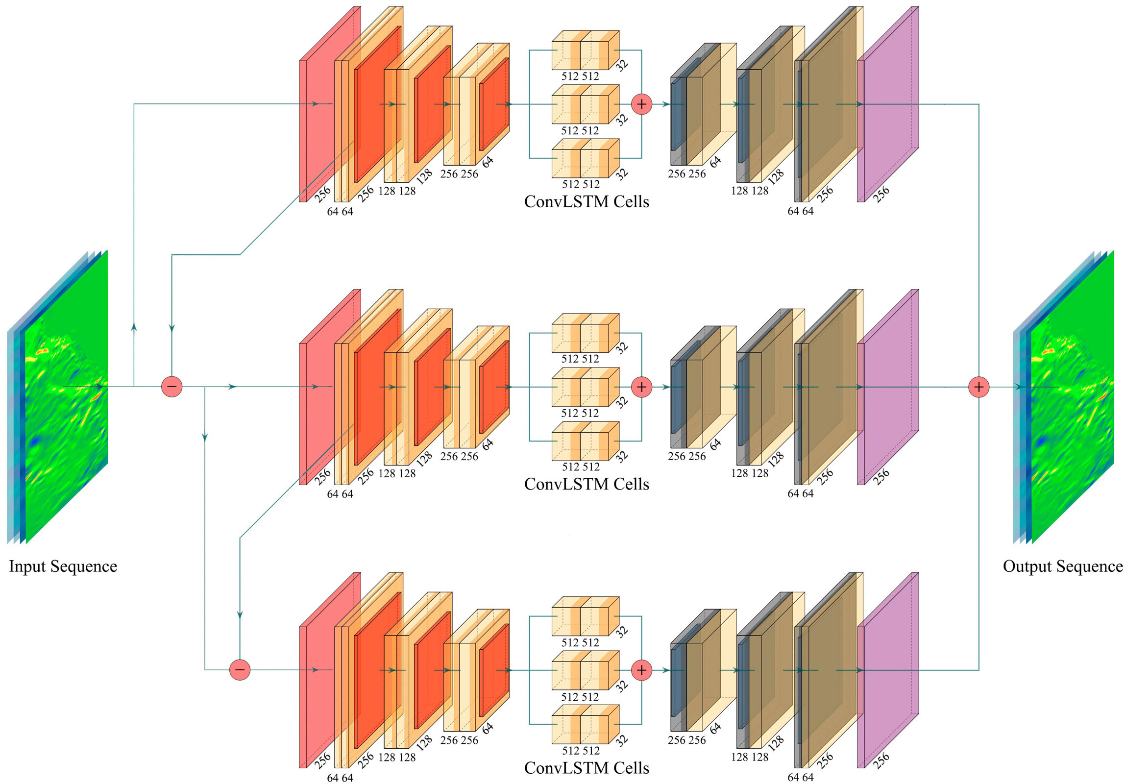
The architecture of our model is shown on the Figure 1. MariNet consists of several interconnected encoder-decoder blocks, within which ConvLSTM modules are embedded between the encoder and the decoder. For this study, we employed four encoder layers and four decoder layers. Each ConvLSTM module contains several parallel ConvLSTM cells connected in a manner that the sum of their outputs forms the resulting forecast of time series in the latent space. This design enables the neural network to simultaneously detect temporal dependencies at various frequencies without assuming any specific frequency distribution and a priori defined data distributions.

Figure 1

Figure 1. The architecture of MariNet.

The encoder-decoder blocks are interconnected in such a way that the input to each subsequent block is the result of subtracting the original data from the original data passed through the first convolutional layer in the block, which produces average pooling. Moreover, the size of the convolution in the first layer of the block varies for each block. This solution facilitates hierarchical pattern highlighting in images: first, the neural network is trained to work with larger patterns. Then it analyzes smaller patterns and their conditional dependencies on larger ones.

During this research, we employed three encoder-decoder architectures. We settled on using three parallel architectures because they enabled us to capture different scales of spatial and temporal variability. The first block learns and captures the largest features, which can be considered as general sea state variability. The second block focuses on large-scale patterns, such as global circulation dynamics. Meanwhile, the third block captures the finest details.

A key feature of the model’s operation is the forecasting algorithm. Unlike typical recursive algorithms, where the forecast from the previous step is cyclically fed into the neural network to form a forecast for the next steps, our neural network sequentially receives several previous values for the water velocity and sea surface heights. When predicting the sea state 3 days ahead with a temporal resolution of 6 hours (i.e., 12 timesteps), we provide the model with 12 consecutive input sequences. Therefore, instead of getting a single array for one time point, our neural network is initialized by the dynamics of such arrays, which allows for a more accurate assessment of the state of the forecasted values, and consequently, ensures a more precise forecast. To train MariNet, we used a learning rate of 0.001, a sigmoid activation function, and the Adam optimizer. The number of training epochs turned out to be 300.

2.2 PhyDNet neural network

PhyDNet is a deep learning model introduced in (Le Guen and Thome, 2020) and designed for unsupervised video prediction. Due to its architecture, the model integrates physical knowledge into the learning process, making it effective for tasks such as weather forecasting, fluid dynamics, and other physical phenomena prediction. The model leverages physical knowledge on dynamics and disentangles it from other unknown factors. To achieve this goal, the authors introduced a PhyDNet disentangling architecture, and PhyCell physically-constrained recurrent cell. The recurrent block projects input video frames into a latent space. This projection is achieved through a deep convolutional encoder, which transforms the input video into a lower-dimensional representation. The latent space is where the disentanglement of physical dynamics and residual information occurs. Two parallel neural networks are responsible for it: PhyCell and ConvLSTM. PhyCell is a recurrent cell that models and solves Partial Differential Equations (PDE) with internal physical predictor computing and combining partial derivatives with convolutions. PhyCell allows exploiting prior physical knowledge to improve prediction of a model, add explainability and leverages physical constraints to limit the number of model parameters. The ConvLSTM network is trained to learn the residuals, or errors, of the physical model’s predictions. By learning these residuals, the network can correct the physical model’s predictions and improve the overall accuracy of the system. Learned physical and residual representations are summed before decoding to predict the future video frame. As a result, PhyDNet generates one-step-ahead prediction that can be extended by recursive feeding predicted frame into the model. It’s important to note that predictions are reinjected as the next input only for the ConvLSTM branch, and not for PhyCell. This is because the PhyCell is designed to capture the deterministic physical dynamics, which should not be influenced by the predictions.

In (Le Guen and Thome, 2020) PhyDNet has been compared with PredRNN, ConvLSTM, Causal LSTM, Memory in Memory (MIM), outperformed them and showed itself as one of the state-of-the-art model of its time. Therefore, we have chosen PhyDNet to compare with our model.

2.3 FourCastNet neural network

FourCastNet, or Fourier ForeCasting Neural Network is first described in (Pathak et al., 2022). It is a data-driven global weather forecasting model that provides short to medium range predictions. It is trained with an ERA5 reanalysis from the European Centre for Medium-Range Weather Forecasts (ECMWF), which has hourly estimates of atmospheric variables at a 0.25° resolution. FourCastNet utilizes a Fourier transform-based token-mixing scheme (Guibas et al., 2021) which is complemented with a vision transformer (ViT) backbone (Dosovitskiy et al., 2021). This method is grounded in the recent advancements in the Fourier neural operator, or Adaptive Fourier Neural Operator (AFNO) that has demonstrated success in modeling challenging partial differential equations (PDE), including fluid dynamics, in a resolution-invariant manner (Li et al., 2020).

According to (Pathak et al., 2022) the use of ViT backbone is preferred due to its ability to effectively model long-range dependencies. The combination of ViT and Fourier-based token mixing produces a model that effectively resolves fine-grained features and scales well with the size and resolution of the dataset, leading to the training of high-fidelity data-driven models at an unprecedented resolution.

The original version of FourCastNet models 20 variables at five vertical levels, that are: surface air pressure, mean sea level pressure, air temperature at 2m from the surface, zonal and meridional wind velocity 10m from the surface; zonal and meridional wind velocity at 1000, 850, and 500 hPa; air temperature at 850 and 500 hPa; geopotential at 1000, 850, 500, and 50hPa; relative humidity at 850 and 500hPa, and Total Column Water Vapor. The authors use the model to predict such variables as the surface wind speed, precipitation, and atmospheric water vapor. They propose FourCastNet to be used for planning wind energy resources, predicting extreme weather events such as tropical cyclones, extra-tropical cyclones, and atmospheric rivers. FourCastNet matches the forecasting accuracy of the ECMWF Integrated Forecasting System (IFS), a state-of-the-art Numerical Weather Prediction (NWP) model, at short lead times for large-scale variables, while outperforming IFS for small-scale variables, including precipitation.

According to (Pathak et al., 2022), the FourCastNet uses such metrics as Root Mean Squared Error (RMSE), Anomaly Correlation Coefficient (ACC) at lead times of up to three days and gives results comparable to the ECMWF Integrated Forecasting System (IFS), considered one of the best classical numerical model used by ECMWF to construct reanalyzes and make weather forecasts.

2.4 Metrics for the model output quality estimation

We trained all three networks with the data on the surface water currents and the sea surface heights, started the inferences and compared their outputs with several metrics: Root Mean Squares Error (RMSE), Bias and Correlation. They are defined as:

$$RMSE=\sqrt{\frac{1}{N}\sum _{i=1}^N{(y_{i }-x_{i })}^2},$$

$$Bias= \frac{1}{N}{\sum }_{i=1}^N{y}_{i }- \frac{1}{N}{\sum }_{i=1}^N{x}_{i, }$$

$$Correlation=\frac{Sxy}{\sqrt{SxxSyy}},\mathrm{w}\mathrm{i}\mathrm{t}\mathrm{h}$$

$$S_{xy}={\sum }_{i=1}^N{x}_{i }{y}_{i }-\frac{{\sum }_{i=1}^N{x}_{i }{\sum }_{i=1}^N{y}_{i }}{N},$$

$$S_{xx}={\sum }_{i=1}^N{x}_i^2 -\frac{{({\sum }_{i=1}^N{x}_i)}^2}{N},$$

$$S_{yy}={\sum }_{i=1}^N{y}_i^2 -\frac{{({\sum }_{i=1}^N{y}_i)}^2}{N},$$

where $x_{i }$is the original data value for a given timestep, $y_{i }$is a predicted value for a given timestep, N – the length of the timeseries.

In scholarly terms, the Root Mean Square Error (RMSE) quantifies the divergence in magnitude between the model’s predictions and the actual observations. It is preferable for the RMSE to be smaller as this signifies a better alignment between predicted and actual values.

Bias, on the other hand, signifies the systematic deviation of the approximated quantifier from the real value and can be interpreted as a consistent overestimation or underestimation of an output. It is desirable for the bias to be closer to zero, indicating that the estimates are nearer to the actual data.

The correlation, in contrast, is a statistical measure that sheds light on the degree to which two variables share a linear relationship. This relationship is frequently deployed to depict the linear association between two contingent factors. Greater values of correlation denote a stronger relationship between the two variables.

3 Data

The Copernicus Marine Environment Monitoring Service (CMEMS) offers a comprehensive global ocean analysis and forecast system through its Global Ocean Physics Analysis and Forecast (CMEMS-GLO-PUM-001-024) product. The system operates at a resolution of 1/12°, updated daily, and provides global ocean forecasts for a 10-day period (Operational Mercator Global Ocean System). The dataset employs a combination of the numerical ocean model NEMO 3.6 with LIM3 Multi-categories sea ice model, ECMWF IFS HRES atmospheric forcing, and several data assimilation techniques, like SAM2 (SEEK Kernel) 4D, allowing for seamless integration of in-situ and satellite observations.

For our needs we choose the region bounded by 60°N-90°N and 5°E-150°W and obtain the hourly surface data of zonal sea water velocity (u), meridional sea water velocity (v), and sea surface height above geoid (zos) for 2019-2022. We interpolate them to the 6-hour temporal resolution and 0.25°x0.25° spatial resolution with and feed the data to the ML models.

4 Results and discussion

The MariNet model demonstrates promising performance. Notably, the figures representing metrics for the FourCastNet model display artifacts. The average metrics are presented in Table 1. As shown in the table, the MariNet model demonstrates minimal RMSE values for sea surface heights and components of surface sea water velocities. Furthermore, the bias of the MariNet model is closest to zero among the mentioned models. Although the mean correlation between models is not significantly high, PhyDNet and MariNet display the highest correlation, approximately 0.5 for sea surface velocities and 0.4 for sea surface heights.

Table 1

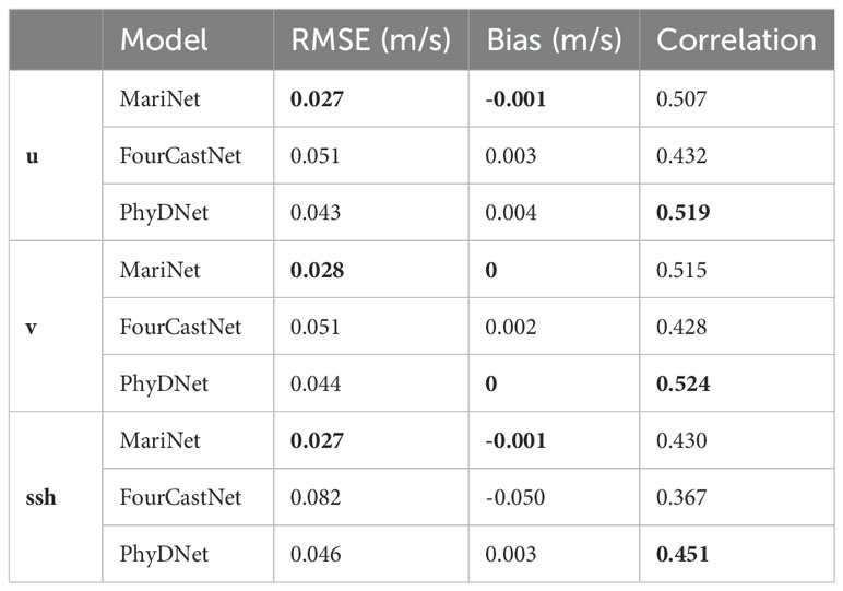
Table 1. Metrics of MariNet, FourCastNet and PhyDNet for zonal and meridional components of surface water velocities and Sea Surface Heights.

Figure 2 illustrates the temporal evolution of RMSE for sea surface velocity and sea surface heights for the selected models throughout the prediction period. As observed, all RMSE values monotonically increase over time. Notably, MariNet and PhyDNet demonstrate comparable results, with their RMSE values growing from approximately 0.01 m/s and 0.01 m to about 0.04 m/s and 0.045 m for sea water velocity and sea surface heights, respectively.

Figure 2

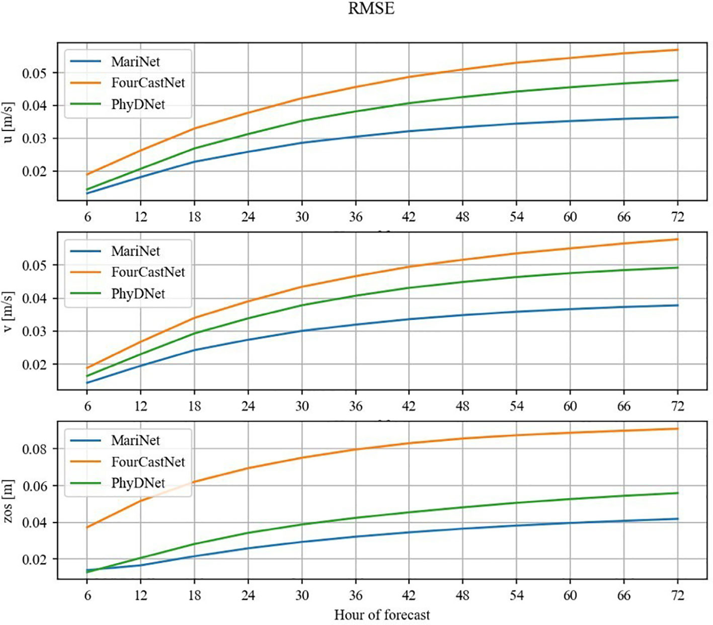
Figure 2. Plots of temporal evolution of RMSE for zonal (upper image), meridional (middle image) components of surface water velocity (m/s), and the sea surface heights (m) above geoid for MariNet (blue line), PhyDNet (green line), and FourCastNet (orange line).

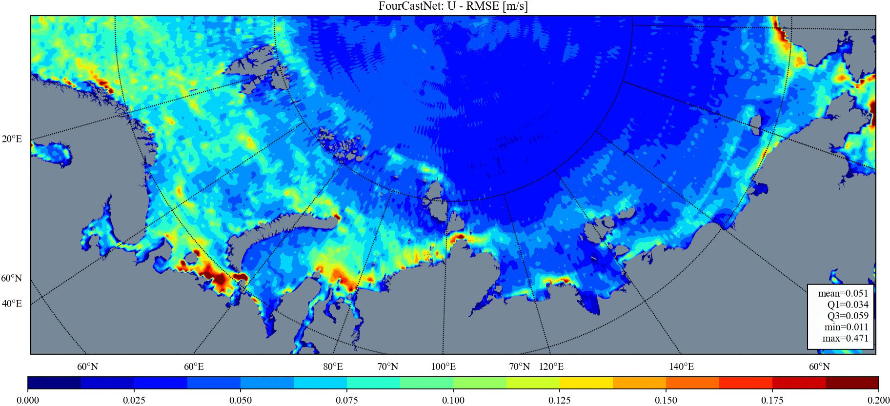
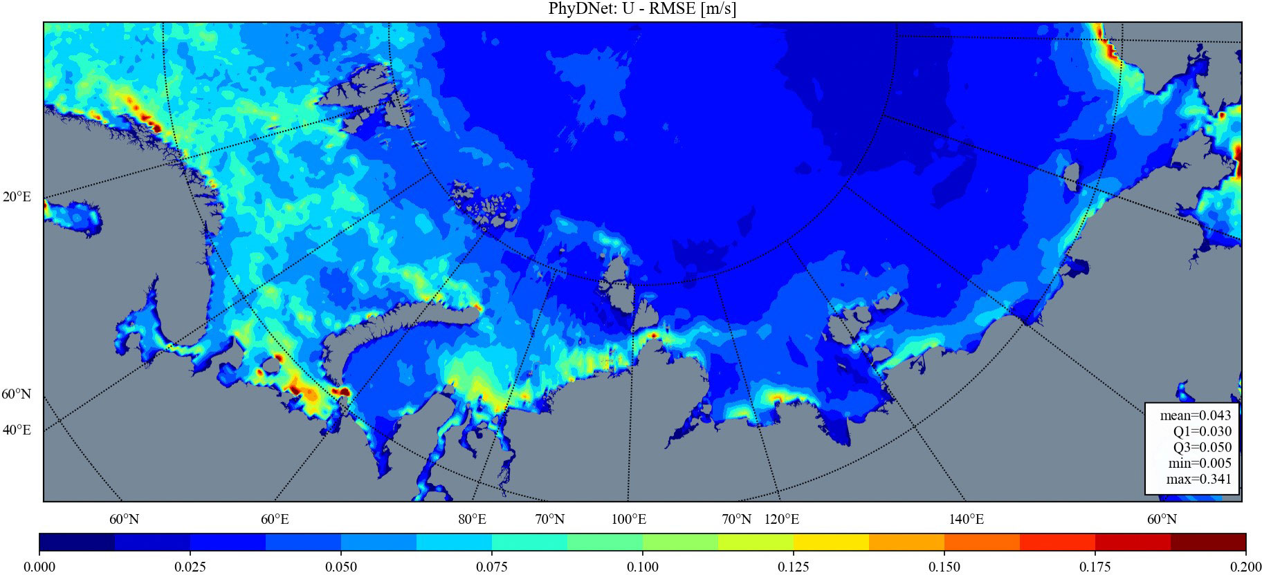
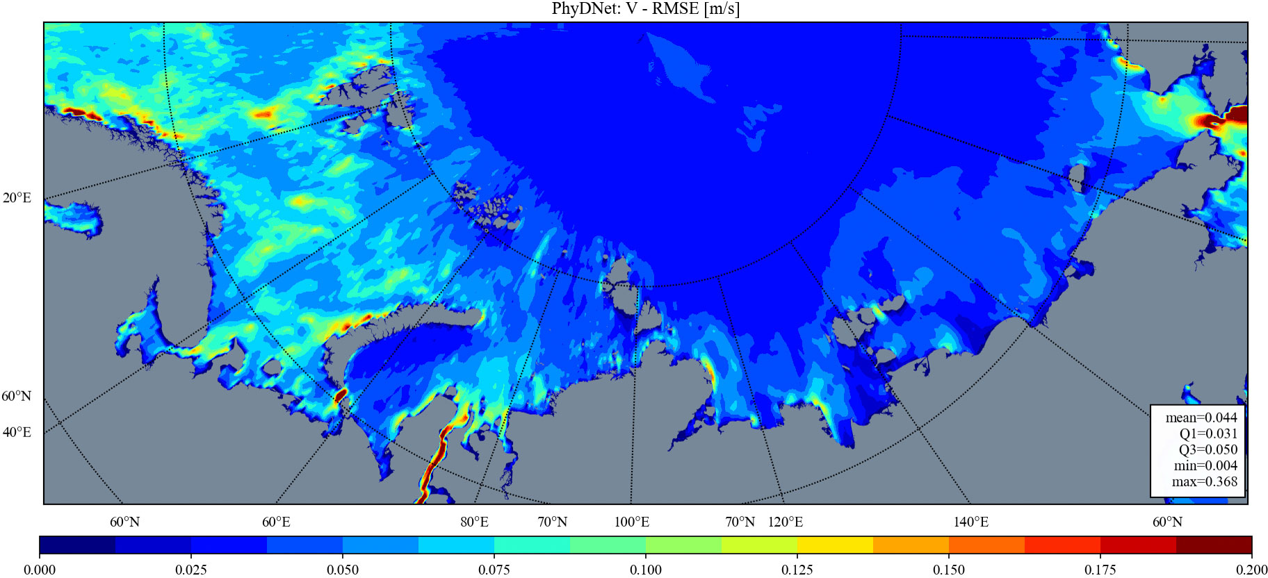
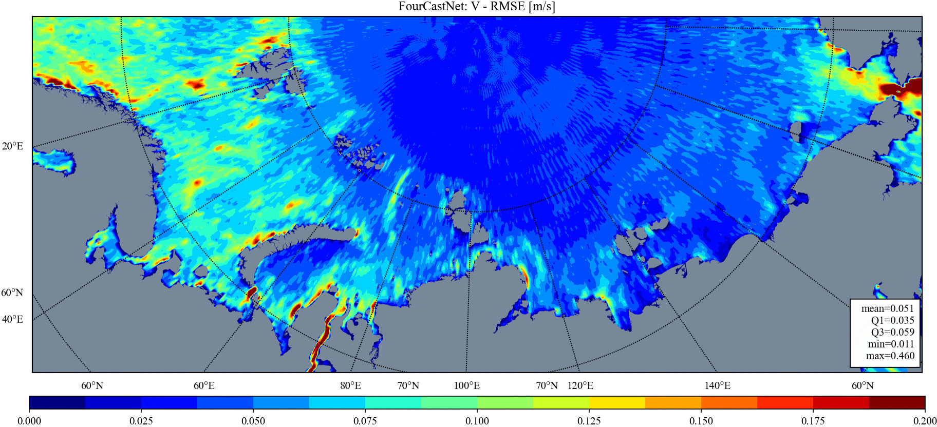
Figures 3–8 depict maps of RMSE for zonal and meridional components of surface water velocity within the research area. All three models exhibit similar spatial distributions of RMSE values, with high values observed in the Barents Sea, Kara Sea, and coastal areas of other seas, as well as low values in eastern offshore regions and the region to the north of the continental shelf. The high RMSE values may be attributed to two primary factors: (1) the model’s poor learning quality or (2) the high standard deviation and variability of the original data. Conversely, the low RMSE values observed in the eastern and northern parts may be due to the relatively low variability of the original water velocity data, with the latter potentially being exacerbated by the presence of sea ice cover in these areas for a significant portion of the year. On the other hand, the high RMSE values in coastal areas could be attributed to the active hydrodynamics in these regions, characterized by larger values and greater variability of the water velocity data.

Figure 3

Figure 3. RMSE (in m/s) for zonal component of the surface water velocity for MariNet model.

Figure 4

Figure 4. RMSE (in m/s) for zonal component of the surface water velocity for FourCastNet model.

Figure 5

Figure 5. RMSE (in m/s) for zonal component of the surface water velocity for PhyDNet model.

Figure 6

Figure 6. RMSE (in m/s) for meridional component of the surface water velocity for MariNet model.

Figure 7

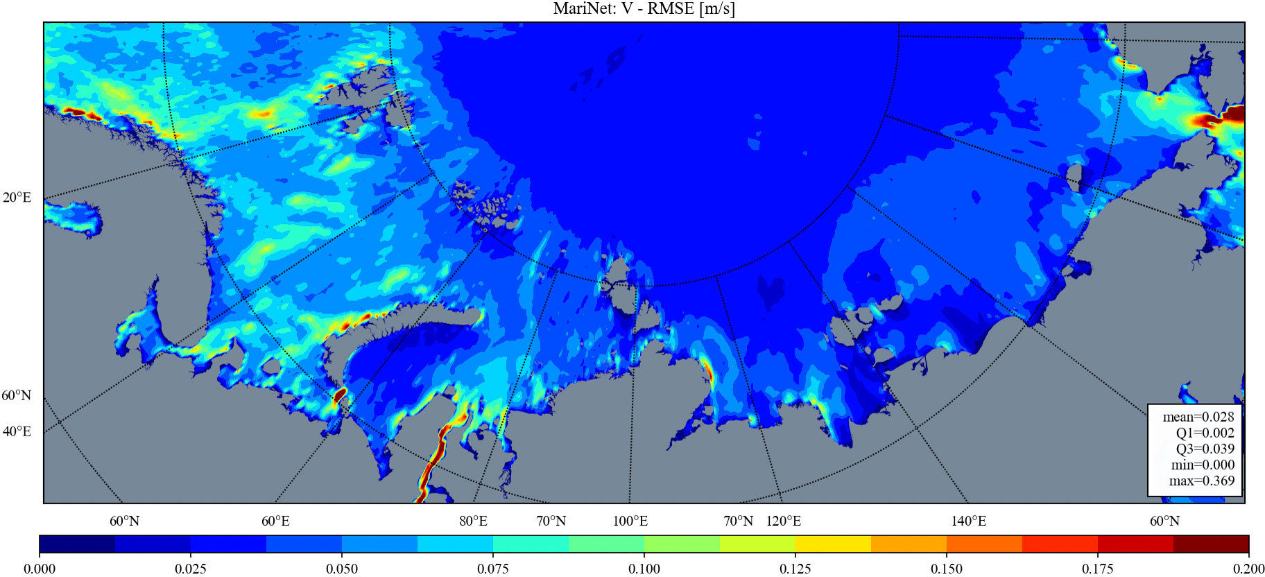
Figure 7. RMSE (in m/s) for meridional component of the surface water velocity for FourCastNet model.

Figure 8

Figure 8. RMSE (in m/s) for meridional component of the surface water velocity for PhyDNet model.

Notably, the general patterns of spatial variability for RMSEs are consistently present across all models’ results; however, MariNet outperforms the other two neural networks in terms of absolute error values. Furthermore, FourCastNet is observed to exhibit artifacts both in zonal and meridional components of surface water velocity. This could indicate that the FourCastNet model fails to accurately capture sea water dynamics patterns.

4.1 Computational cost of MariNet

With the CodeCarbon software package, we have calculated the carbon emissions and the energy consumption of the MariNet, FourCastNet and the PhyDNet for our calculations. Results are shown in the Table 2. Training of the MariNet model has the least carbon emission rate, but, due to the relatively large time of training, it takes the most energy. At the same time, PhyDNet wins the energy consumption and the emission rate challenges.

Table 2

Table 2. Comparison of the carbon emissions and energy consumption during the models training and inference.

5 Conclusions

In the study, we proposed a forecast model MariNet model, based on the encoder-decoder architecture, and compared it with FourCastNet and PhyDNet, the most promising ML models in the field weather prediction of their time. We have chosen the Arctic region, one of the hottest spots of the modern climate science research and obtained the hourly data on zonal and meridional velocities of the surface sea water and sea surface heights above geoid from the Copernicus Marine Data Store. We switched temporal resolution from 1 hour to 6 hours and fed the datasets to the MariNet model, PhyDNet and FourCastNet.

In comparison with the other mentioned ML models, the RMSE and bias of the MariNet model are significantly lower. At the same time, the mean correlations of all three models with the original data are moderate and located between 0.4-0.5.

The above experimental results all show that the MariNet model has great potential in the mid-term predictions of the ocean dynamics. The further development of the model incudes improving the efficiency of computational operations, expanding the number of parallel running modules of our model to capture more temporal and spatial features of data variability, and increase the number of variables used in training.

Data availability statement

The original contributions presented in the study are included in the article/Supplementary Material. Further inquiries can be directed to the corresponding author.

Author contributions

AB: Conceptualization, Data curation, Formal Analysis, Investigation, Writing – original draft. DI: Investigation, Methodology, Software, Validation, Visualization, Writing – review & editing. EN: Conceptualization, Investigation, Methodology, Software, Visualization, Writing – review & editing. AE: Funding acquisition, Project administration, Supervision, Writing – review & editing. PI: Funding acquisition, Project administration, Resources, Supervision, Writing – review & editing. NS: Conceptualization, Formal Analysis, Investigation, Supervision, Writing – review & editing.

Funding

The author(s) declare that financial support was received for the research, authorship, and/or publication of this article. The research was funded under a grant for implementing a pilot project aimed at testing artificial intelligence technologies in priority industries as a part of the federal project ‘Artificial Intelligence’ within the national program ‘Digital Economy of the Russian Federation’.

Acknowledgments

The study has been conducted using E.U. Copernicus Marine Service Information; https://doi.org/10.48670/moi-00016. We would like to acknowledge the use of the GitHub repository https://github.com/nvlabs/fourcastnet for providing the FourCastNet code, https://github.com/vincent-leguen/PhyDNet for providing the PhyDNet code used in our experiments, and https://github.com/mlco2/codecarbon for the CodeCarbon package.

Conflict of interest

Authors AB, DI, EN, and NS were employed by the company Marine Information Technologies LLC.

The remaining authors declare that the research was conducted in the absence of any commercial or financial relationships that could be construed as a potential conflict of interest.

Publisher’s note

All claims expressed in this article are solely those of the authors and do not necessarily represent those of their affiliated organizations, or those of the publisher, the editors and the reviewers. Any product that may be evaluated in this article, or claim that may be made by its manufacturer, is not guaranteed or endorsed by the publisher.

References

Bjerknes V. (1904). Das Problem der Wettervorhersage, betrachtet vom Standpunkte der Mechanik und der Physik. Meterologische Z. Wien, Vol. 21, 1–7.

Google Scholar

Bjerknes V. (1914). Meteorology as an exact science. Monthly Weather Review 42 (1), 11–14. Available online at: https://journals.ametsoc.org/view/journals/mwre/42/1/1520-0493_1914_42_11_maaes_2_0_co_2.xml (Accessed October 18, 2024).

Google Scholar

Bryan K. (1969). Climate and the ocean circulation: III. The ocean model. Mon. Weather Rev. 97, 806–827. doi: 10.1175/1520-0493(1969)097<0806:CATOC>2.3.CO;2

Crossref Full Text | Google Scholar

Buinyi A., Irishev D., Nikulin E., Evdokimov A., Sukhikh N. (2023). On the machine learning experience for the ocean circulation modeling and forecast in the arctic ocean. Conference Poster. doi: 10.13140/RG.2.2.23386.31686

Crossref Full Text | Google Scholar

Buinyi A., Zhdanova E., Evdokimov A., Sukhikh N. (2022). On the artificial intelligence for the sea state forecast along the northern sea route. Int. J. Offshore Polar Eng. 32, 411–417. doi: 10.17736/ijope.2022.jc870

Crossref Full Text | Google Scholar

Chen C., Gao G., Qi J., Proshutinsky A., Beardsley R. C., Kowalik Z., et al. (2009). A new high-resolution unstructured grid finite volume Arctic Ocean model (AO-FVCOM): An application for tidal studies. J. Geophys. Res. 114, C08017. doi: 10.1029/2008JC004941

Crossref Full Text | Google Scholar

Dong C., Xu G., Han G., Bethel B. J., Xie W., Zhou S. (2022). Recent developments in artificial intelligence in oceanography. Ocean-Land-Atmosphere Res. doi: 10.34133/2022/9870950

Crossref Full Text | Google Scholar

Dosovitskiy A., Beyer L., Kolesnikov A., Weissenborn D., Zhai X., Unterthiner T., et al. (2021). An image is worth 16x16 words: transformers for image recognition at scale. arXiv preprint. doi: 10.48550/arXiv.2010.11929

Crossref Full Text | Google Scholar

Du Y., Song W., He Q., Huang D., Liotta A., Su C. (2019). Deep learning with multi-scale feature fusion in remote sensing for automatic oceanic eddy detection. Inf. Fusion 49, 89–99. doi: 10.1016/j.inffus.2018.09.006

Crossref Full Text | Google Scholar

Duo Z., Wang W., Wang H. (2019). Oceanic mesoscale eddy detection method based on deep learning. Remote Sens. 11, 1921. doi: 10.3390/rs11161921

Crossref Full Text | Google Scholar

Fan S., Xiao N., Dong S. (2020). A novel model to predict significant wave height based on long short-term memory network. Ocean Eng. 205, 107298. doi: 10.1016/j.oceaneng.2020.107298

Crossref Full Text | Google Scholar

Franz K., Roscher R., Milioto A., Wenzel S., Kusche J. (2018). “Ocean eddy identification and tracking using neural networks,” in IGARSS 2018 - 2018 IEEE International Geoscience and Remote Sensing Symposium, Valencia, Spain. 6887–6890 (New York, NY: IEEE). doi: 10.1109/IGARSS.2018.8519261

Crossref Full Text | Google Scholar

Fuentes A. G., Nicolis O., Peralta B., Chiodi M. (2021). “ConvLSTM Neural Networks for seismic event prediction in Chile,” in 2021 IEEE XXVIII International Conference on Electronics, Electrical Engineering and Computing (INTERCON), Lima, Peru. 1–4 (New York, NY: IEEE). doi: 10.1109/INTERCON52678.2021.9532946

Crossref Full Text | Google Scholar

Gao S., Huang J., Li Y., Liu G., Bi F., Bai Z. (2021). A forecasting model for wave heights based on a long short-term memory neural network. Acta Oceanol. Sin. 40, 62–69. doi: 10.1007/s13131-020-1680-3

Crossref Full Text | Google Scholar

Guibas J., Mardani M., Li Z.-Y., Tao A., Anandkumar A., Catanzaro B. (2021). Adaptive fourier neural operators: efficient token mixers for transformers. ArXiv. doi: 10.48550/arXiv.2111.13587

Crossref Full Text | Google Scholar

Halley E. (1686). An historical account of the trade winds, and monsoons, observable in the seas between and near the Tropicks, with an attempt to assign the physical cause of the said winds. Philos. Trans. R. Soc Lond. 16, 153–168. doi: 10.1098/rstl.1686.0026

Crossref Full Text | Google Scholar

Le Guen V., Thome N. (2020). “Disentangling physical dynamics from unknown factors for unsupervised video prediction,” in 2020 IEEE/CVF Conference on Computer Vision and Pattern Recognition (CVPR), Seattle, WA, USA. 11471–11481 (New York, NY: IEEE). doi: 10.1109/CVPR42600.2020.01149

Crossref Full Text | Google Scholar

Lguensat R., Sun M., Fablet R., Tandeo P., Mason E., Chen G. (2018). “EddyNet: A deep neural network for pixel-wise classification of oceanic eddies,” in IGARSS 2018 - 2018 IEEE International Geoscience and Remote Sensing Symposium, Valencia. 1764–1767 (New York, NY: IEEE). doi: 10.1109/IGARSS.2018.8518411

Crossref Full Text | Google Scholar

Li Z., Kovachki N., Azizzadenesheli K., Liu B., Bhattacharya K., Stuart A., et al. (2020). Fourier neural operator for parametric partial differential equations. arXiv preprint. doi: 10.48550/ARXIV.2010.08895

Crossref Full Text | Google Scholar

Lin H., Hua Y., Ma L., Chen L. (2019). “Application of convLSTM network in numerical temperature prediction interpretation,” in Proceedings of the 2019 11th International Conference on Machine Learning and Computing, New York, NY, USA. 109–113 (New York, NY, USA: Association for Computing Machinery). doi: 10.1145/3318299.3318381

Crossref Full Text | Google Scholar

Ling F., Luo J.-J., Li Y., Tang T., Bai L., Ouyang W., et al. (2022). Multi-task machine learning improves multi-seasonal prediction of the Indian Ocean Dipole. Nat. Commun. 13, 7681. doi: 10.1038/s41467-022-35412-0

PubMed Abstract | Crossref Full Text | Google Scholar

Liu Q., Zhang R., Wang Y., Yan H., Hong M. (2021). Daily prediction of the arctic sea ice concentration using reanalysis data based on a convolutional lstm network. J. Mar. Sci. Eng. 9. doi: 10.3390/jmse9030330

Crossref Full Text | Google Scholar

Mandal S., Prabaharan N. (2006). Ocean wave forecasting using recurrent neural networks. Ocean Eng. 33, 1401–1410. doi: 10.1016/j.oceaneng.2005.08.007

Crossref Full Text | Google Scholar

Maury M. F. (1855). The physical geography of the sea (London: Sampson, Low, Son & Co). doi: 10.5962/bhl.title.102148

Crossref Full Text | Google Scholar

Moishin M., Deo R. C., Prasad R., Raj N., Abdulla S. (2021). Designing deep-based learning flood forecast model with ConvLSTM hybrid algorithm. IEEE Access 9, 50982–50993. doi: 10.1109/ACCESS.2021.3065939

Crossref Full Text | Google Scholar

Navier C. L. M. H. (1822). Mémoire sur les lois mouvement des fluides. Mem Acad. Sci. Inst Fr 6, 389–440. Available online at: https://fr.wikisource.org/wiki/Page:M%C3%A9moires_de_l%E2%80%99Acad%C3%A9mie_des_sciences,_Tome_6.djvu/577 (accessed October 18, 2024).

Google Scholar

Ning P., Zhang C., Zhang X., Jiang X. (2021). Short- to medium-term sea surface height prediction in the bohai sea using an optimized simple recurrent unit deep network. Front. Mar. Sci. 8. doi: 10.3389/fmars.2021.672280

Crossref Full Text | Google Scholar

Pathak J., Subramanian S., Harrington P., Raja S., Chattopadhyay A., Mardani M., et al. (2022). Fourcastnet: A global data-driven high-resolution weather model using adaptive fourier neural operators. arXiv preprint. doi: 10.48550/ARXIV.2202.11214

Crossref Full Text | Google Scholar

Richardson L. (1922). Weather Prediction by Numerical Process. Cambridge: Cambridge University Press.

Google Scholar

Robinson A. R. (1983). “Overview and summary of eddy science,” in Eddies in Marine Science. Ed. Robinson A. R. (Springer Berlin Heidelberg, Berlin, Heidelberg), 3–15. doi: 10.1007/978-3-642-69003-7_1

Crossref Full Text | Google Scholar

Santana O., Hernández-Sosa D., Martz J., Smith R. (2020). Neural network training for the detection and classification of oceanic mesoscale eddies. Remote Sens. 12, 2625. doi: 10.3390/rs12162625

Crossref Full Text | Google Scholar

Shi X., Chen Z., Wang H., Yeung D. Y., Wong W.-K., Woo W. (2015). Convolutional LSTM network: A machine learning approach for precipitation nowcasting. NIPS. 28, 802–810. Available online at: https://proceedings.neurips.cc/paper_files/paper/2015/file/07563a3fe3bbe7e3ba84431ad9d055af-Paper.pdf (accessed October 18, 2024).

Google Scholar

Song T., Han N., Zhu Y., Li Z., Li Y., Li S., et al. (2021). Application of deep learning technique to the sea surface height prediction in the South China Sea. Acta Oceanol. Sin. 40, 68–76. doi: 10.1007/s13131-021-1735-0

Crossref Full Text | Google Scholar

Stokes G. (1845). On the theories of the internal friction of fluids in motion. Trans. Camb. Philos. Soc 8, 287–319.

Google Scholar

Storto A., Alvera-Azcárate A., Balmaseda M. A., Barth A., Chevallier M., Counillon F., et al. (2019). Ocean reanalyses: recent advances and unsolved challenges. Front. Mar. Sci. 6. doi: 10.3389/fmars.2019.00418

Crossref Full Text | Google Scholar

Sverdrup H. U., Munk W. H. (1947). Wind, sea and swell: Theory of relations for forecasting (No. 601). Hydrographic Office. Available online at: https://api.semanticscholar.org/CorpusID:132860343. (accessed October 18, 2024).

Google Scholar

Xu G., Cheng C., Yang W., Xie W., Kong L., Hang R., et al. (2019). Oceanic eddy identification using an AI scheme. Remote Sens. 11, 1349. doi: 10.3390/rs11111349

Crossref Full Text | Google Scholar

Xu G., Xie W., Dong C., Gao X. (2021). Application of three deep learning schemes into oceanic eddy detection. Front. Mar. Sci. 8. doi: 10.3389/fmars.2021.672334

Crossref Full Text | Google Scholar

Zhou S., Bethel B. J., Sun W., Zhao Y., Xie W., Dong C. (2021). Improving significant wave height forecasts using a joint empirical mode decomposition–long short-term memory network. J. Mar. Sci. Eng. 9, 744. doi: 10.3390/jmse9070744

Crossref Full Text | Google Scholar

Zulfa I. I., Novitasari D. C. R., Setiawan F., Fanani A., Hafiyusholeh M. (2021). Prediction of sea surface current velocity and direction using LSTM. IJEIS Indones. J. Electron. Instrum. Syst. 11, 93. doi: 10.22146/ijeis.63669

Crossref Full Text | Google Scholar