Laboratory study of energy transformation characteristics in breaking wave groups

The spilling-breaking waves that appear in chirped wave packets are studied in a two-dimensional wave channel. These waves are produced by superposing waves with gradually decreasing frequencies. The analysis focuses on the nonlinear characteristics, energy variation, and energy transformation during the evolution and breaking of wave groups. Ensemble empirical mode decomposition is used to analyze the non-breaking and breaking energy variations of the intrinsic mode functions (IMFs). It is found that the third-order IMF component is a source of non-breaking energy dissipation and the second-order IMF, which represents a short wave group with a relatively higher energy content, is a primary source of the energy loss caused by wave breaking. Additionally, the findings reveal that among the three waves preceding the maximum crest, the wave closest to the maximum crest carried most of the energy. When wave breaking occurs, the energy dissipation caused by the wave breaking primarily originates from that wave. After wave breaking, whether it is the first breaker or subsequent breakers, the main energy dissipation occurs in a frequency range higher than the dominant frequency. This energy loss plays a significant role in increasing the energy of free waves. Moreover, a potential link between the number of carrier waves and wave breaking phenomena has been found. As the number of carrier waves increased, both the nonbreaking and breaking energy dissipation rates exhibited an overall increasing trend. The amount of nonbreaking energy dissipation was generally more than twice the breaking energy dissipation rate. For wave groups with more carrier waves, the modulation instability plays a significant role in generating larger waves. Furthermore, an analysis of the dominant frequency variations of the wave group before wave breaking suggests that wave breaking is not a sufficient condition for a frequency downshift in the wave spectra.

Introduction

Breaking waves pose a significant and unpredictable threat to human life and oceanic structures (He et al., 2023a; Onorato et al., 2006; Porubov et al., 2005; Toffoli et al., 2011; Trulsen et al., 2020; Viotti and Dias, 2014), leading to serious consequences. Before wave breaking occurs, when a wave reaches a local maximum, it is often referred to as an extreme wave. During the complex process of focusing and breaking, significant changes occur in the wave nonlinearity. This is a crucial characteristic of water waves and is used to describe various oceanic phenomena, such as extreme events (Fu et al., 2021, 2022; Luo et al., 2022; Ma et al., 2020; Veltcheva and Soares, 2016; Zhang and Benoit, 2021), energy distribution and transformation (Gao et al., 2024b; Gibson and Swan, 2007; Mahmoudof et al., 2016; Mahmoudof and Hajivalie, 2021), wave breaking (Banner and Peirson, 2007; He et al., 2022; Tian et al., 2010; Zhao and Sun, 2010), convective hybrid nanofluid flow (Zhang et al., 2022b), and harbor resonance (Gao et al., 2024a, Gao et al., 2021, Gao et al., 2023; Wang et al., 2022). Therefore, it is crucial to study the nonlinear characteristics of extreme and breaking waves during wave evolution to understand the underlying dynamic processes. This has significant implications for the design of oceanic structures (Buldakov et al., 2017).

Wave breaking is a result of wave energy focusing, and often occurs at the envelope maxima of wave groups (Holthuijsen and Herbers, 1986). These locations tend to coincide with the occurrence of extreme waves. Various physical mechanisms have been demonstrated to contribute to the generation of extreme waves, such as dispersion focusing (Rapp and Melville, 1990), modulation instability (Ma et al., 2012; Onuki and Hibiya, 2019), spatial focusing (Peregrine, 1976), interactions between wave groups (Fu et al., 2022; Wang et al., 2020; Zhou et al., 2023), wave-current interactions (Chen and Zou, 2017) and non-equilibrium dynamics (Chen et al., 2024; He et al., 2023b; Trulsen et al., 2020, Trulsen et al., 2012; Zhang et al., 2022a). However, considering all mechanisms responsible for generating extreme waves and analyzing their nonlinear evolutionary characteristics can be challenging. When the water depth is constant, the nonlinear hydrodynamic effect associated with the energy and momentum fluxes within the deforming wave groups becomes the primary determining factor (Babanin et al., 2001). Therefore, this study primarily focuses on analyzing the nonlinearity and energy transformation of extreme waves and their subsequent breaking waves by combining the mechanisms of dispersion focusing and modulation instability in generating wave groups.

Studying the nonlinear evolutionary process of a single-wave group is an appropriate approach to determine the underlying characteristics of extreme waves and nonlinear processes during wave breaking. When an extreme wave reaches its limit, wave breaking occurs, resulting in significant energy losses, noticeable energy transformations, and intense nonlinear interactions. Numerous numerical and experimental investigations have been conducted to provide valuable insights into this phenomenon. During the evolution of wave groups towards extreme conditions, nonlinearity causes notable variations in wave energy (Rapp and Melville, 1990; Wu and Yao, 2004). Liang et al. (2017) conducted experimental studies on wave breaking and examined variations in wave energy through the energy spectrum. They demonstrated that the energy concentrated near the high-frequency components dissipated, whereas the energy around the peak frequency increased during wave breaking. Buldakov et al. (2017) employed a novel method for generating wave groups to investigate the nonlinear characteristics of extreme waves. They found that the spectral properties of waves were closely related to the wave breaking behavior. Dong et al. (2020) investigated the energy properties of waves with varying degrees of nonlinearity and demonstrated that as the wave nonlinearity increased, the energy distribution within the waves became more uneven. Wu and Yao (2004) experimentally investigated the effect of the spectral slope on the degree of energy transformation when extreme waves appear. Their results indicated that the energy transformation towards higher frequencies in the spectrum can indicate the occurrence of extreme waves. Although previous studies have provided valuable insights into the wave energies of extreme and breaking waves, there is still a clear need to understand the local nonlinear transformation process as waves evolve to the local maximum and subsequently break. The nonlinear interactions and underlying components of energy loss require further clarification.

The application of the fast Fourier transform (FFT) linear method has produced numerous results, with a focus on essential components characterized by constant amplitudes and frequencies. However, it is important to note that real oceanic waves are nonlinear and unstable, making it inappropriate to approximate nonlinearity using linearity. Therefore, employing signal processing methods suitable for nonlinear and nonstationary data analysis is crucial for accurately determining the intrinsic characteristics of a signal. Several researchers have achieved noteworthy results by employing wavelet analysis (Abroug et al., 2020; Dong et al., 2008a, Dong et al., 2008b; Fu et al., 2022; Veltcheva and Guedes Soares, 2015; Wang et al., 2020) and the Hilbert-Huang transform (HHT) (He et al., 2023a; Malila et al., 2022; Veltcheva and Soares, 2016; Veltcheva and Guedes Soares, 2016) methods. However, most research has primarily focused on the wave-breaking criteria, wave groupiness, and geometric characteristics, with fewer investigations conducted to analyze the local energy variations of the underlying components. Therefore, in this study, a comprehensive analysis involving HHT, wavelet-based bicoherence, and FFT is employed to study the nonlinear local process during wave breaking.

Real oceanic waves exhibit grouping during their evolution, and studying the nonlinear characteristics of wave groups provides a better understanding of the essential features of extreme waves. To better represent actual sea conditions, in this study, wave groups are generated experimentally without the focusing location being predetermined. The remainder of this paper is organized as follows: Section 2 describes the data processing methods, Section 3 presents the experimental setup and case conditions, Section 4 presents the results of the study, and Section 5 presents the discussion and conclusions.

Materials and methods

Hilbert-Huang transform method

In this study, HHT proposed by Huang et al. (1998) was used to analyze experimental records. HHT is composed of empirical mode decomposition (EMD) and the Hilbert transform (HT). To solve the mode mixing problem that may occur when the narrowband signal was decomposed by EMD and to effectively extract the intrinsic mode functions (IMFs), ensemble empirical mode decomposition (EEMD) was used in the decomposition step of HHT in this study. Because EEMD is a modification of EMD, in this study, a brief introduction to EMD is provided first and then a concise overview of EEMD is presented. According to Huang et al. (1998) and Wu and Huang (2008), a data record x(t) can be decomposed into several intrinsic mode functions and a residual (R) using EMD:

$\begin{array}{ll}x(t)={\displaystyle \sum _{j=1}^n{c}_j}(t)+R.& (1)\end{array}$

In Equation 1, c_j(t) represents the j_th order IMF. For each IMF, the Hilbert transform C_j(t) is:

$\begin{array}{ll}{C}_j(t)=\frac{1}{\pi }P{\displaystyle {\int }_{-\infty }^{+\infty }\frac{c_j(t^{\text{'}})}{t-t^{\text{'}}}}d{t}^{\text{'}},& (2)\end{array}$

where P denotes Cauchy’s principal value. Accordingly, the analytical function Z_j(t) can be expressed as

$\begin{array}{ll}{Z}_j(t)=c_j(t)+i{C}_j(t)=a_j(t)e^{i{\theta }_j(t)},& (3)\end{array}$

where the instantaneous amplitude a_j(t) and phase θ_j(t) are denoted as:

$\begin{array}{ll}{a}_j(t)=\sqrt{c_j^2(t)+C_j^2(t)},{\theta }_j(t)=\arctan \left(\frac{C_j(t)}{c_j(t)}\right).& (4)\end{array}$

The instantaneous angular frequency ω_j(t) can be obtained by differentiating θ_j(t):

$\begin{array}{ll}{\omega }_j(t)=\frac{d{\theta }_j(t)}{dt},& (5)\end{array}$

the corresponding instantaneous frequency f(t) = ω(t)/2π. Therefore, the original data record x(t) can be expressed as:

$\begin{array}{ll}x(t)=\Re \left({\displaystyle \sum _{j=1}^n{a}_j(t)e^{\left(i{\displaystyle \int {\omega }_j(t)dt}\right)}}\right)& (6)\end{array}$

where ℜ represents the real part. The above is the decomposition process of EMD.

For EEMD, multiple “artificial” signals can be generated for x(t) by incorporating white noise into the signal. The k_th “artificial” signal can be expressed as follows:

$\begin{array}{ll}{x}_k(t)=x(t)+n_k(t),& (7)\end{array}$

where n_k(t) represents the k_th addition of white noise to the original signal. By applying EMD to x_k(t) for component decomposition, the following expression is obtained:

$\begin{array}{ll}{x}_k(t)={{\displaystyle \sum _{j=1}^n(c_j(t))}}_k+R_k.& (8)\end{array}$

Referring to the research findings of Wu and Huang (2008), it is sufficient to add white noise N = 300 times to satisfy the requirements for reasonable decomposition. The j_th IMF, c_j(t), can be refined as:

$\begin{array}{ll}{c}_j(t)={\displaystyle \sum _{k=1}^N\frac{{(c_j(t))}_k}{N}.}& (9)\end{array}$

For each IMF obtained by Equation 9, the operations described from Equation 2 to Equation 5 are performed. Finally, according to Equation 6, the time-frequency distribution of energy (square of amplitude) H²(f, t) can be obtained. The instantaneous energy, IE(t), can be obtained by integrating the energy over the frequency range:

$\begin{array}{ll}IE(t)={\displaystyle {\int }_f{H}^2(f,t)}df.& (10)\end{array}$

By integrating the instantaneous energy over time, the energy associated with the wave surface elevation, which refers to the potential energy, can be obtained. According to Tian et al. (2010), the total energy can be obtained by integrating the energy flux F(x, t), which is defined as:

$\begin{array}{ll}F(x,t)=\rho g{C}_{\text{gs}}{\eta }^2(x,t),& (11)\end{array}$

where ρ is the water mass density; g is the gravitational acceleration; and C_gs is the spectrally weighted group velocity computed with surface elevation measurements at the first wave station, and defined as:

$\begin{array}{ll}{C}_{\text{gs}}=\frac{{\displaystyle \sum (C_{\text{gn}}{a}_{\text{n}}^2){(\Delta f)}_{\text{n}}}}{{\displaystyle \sum (a_{\text{n}}^2){(\Delta f)}_{\text{n}}}},& (12)\end{array}$

where C_gn and a_n are the linear group velocity and amplitude of the nth component of the wave train, respectively, and (Δf)_n is the frequency difference between components, which is constant. Although the parameter C_gs may change under different wave conditions, it remains constant for each specific wave condition. Based on Equations 11 and 12, the relationship between the total energy and potential energy can be regarded as a constant ratio. This study focused primarily on the process of spectral evolution, spectral changes, and energy dissipation rates for breaking and non-breaking wave groups. Therefore, it was considered that this constant did not affect the energy variation trend or the energy dissipation rate, for the constant in percentage can be cancelled out when considering the energy dissipation using it as a reference baseline. Thus, similar to the study conducted by Veltcheva and Guedes Soares (2016), the energy characteristics during the wave propagation process were analyzed based on the potential energy obtained through the time integration of the instantaneous energy IE(t).

Before analyzing the energy evolution involving wave breaking, it is necessary to explain the determination of the breaking location. Before starting the experiment, several workers were positioned alongside the water tank, with each person standing approximately 1-2 m apart. Their task was to mark the locations and times at which breakers were observed. The wave propagation process was simultaneously recorded. By analyzing the recorded positions of wave breaking and correlating them with the time and location data captured in the footage, the approximate locations of wave breaking were determined. These positions, combined with changes in the collected data, such as a decrease in the wave surface elevation after reaching its maximum, were used to determine the wave breaking locations. As waves evolve and break, their energy decreases significantly, and the breaking process gradually diminishes. The end of the breaking region is defined as the point at which whitecaps no longer appear. Thus, the locations between the first appearance and the last disappearance of whitecaps formed the approximate boundaries for the breaking region. However, owing to the limitations of the experiment, there were gaps between the installation positions of the wave gauges. This implies that there was a possibility that the locations at which breaking initiated and ceased did not align precisely with the positions of the wave gauges. Consequently, some breakers may have remained undetected if no wave gauge was installed at that specific location. In particular, for highly nonlinear wave conditions, multiple instances of breaking can occur during the evolution. Therefore, breaking events that did not occur at the measurement points were not considered in this study. All the breaking events analyzed in this study are based on data collected by the wave gauges.

Wave-based bicoherence

Wave-based bicoherence is often used to study the nonlinear phase-coupling process during wave evolution (Abroug et al., 2020). For a measured data record x(t), the continual wavelet transform WT (a, τ) can be expressed as (Chen et al., 2018; Dong et al., 2008b):

$\begin{array}{ll}WT(a,\tau )={\displaystyle {\int }_{-\infty }^{\infty }x(t)}{\psi }_{a,\tau }^{*}(t)dt,& (13)\end{array}$

where the asterisk denotes the complex conjugate, and the notation ψ_a,τ (t) represents a family of functions known as wavelets. These wavelet functions are constructed by translating in time τ and dilation with scale a, where a is inversely related to the frequency f. In this study, the Morlet wavelet was selected as the “mother” wavelet function ψ (t), and the expression for ψ_a,τ (t) can be given as follows:

$\begin{array}{ll}{\psi }_{a,\tau }(t)={\left|a\right|}^{-0.5}\psi \left(\frac{t-\tau }{a}\right).& (14)\end{array}$

According to Ma et al. (2017), the wavelet-based bispectrum B(f₁, f₂) is defined as follows:

$\begin{array}{ll}B(f_1,f_2)={\displaystyle {\int }_{T}WT(f_1,\tau )}WT(f_2,\tau )W{T}^{*}(f,\tau )d\tau & (15)\end{array}$

where T is the time duration, and f₁ and f₂ are frequencies that satisfy the relationship f = f₁ + f₂. The wavelet-based bispectrum measures the correlation between f₁, f₂ and f₁ + f₂ using the same process. In this study, the normalized squared wavelet-based bicoherence b² was utilized to quantify the degree of nonlinear phase-coupling interactions. It is defined as:

$\begin{array}{ll}{b}^2(f_1,f_2)=\frac{{\left|B(f_1,f_2)\right|}^2}{\left[{\displaystyle {\int }_T{\left|WT(f_1,t)WT(f_2,t)\right|}^{2}dt}\right]{\displaystyle {\int }_T{\left|WT(f,t)\right|}^{2}dt}}& (16)\end{array}$

According to Equations 15 and 16, the normalized squared wavelet-based bicoherence b² has a value ranging between 0 and 1: b² = 0 indicates a random phase-coupling relationship between wave triads. However, b² = 1 signifies the maximum degree of coupling between triads. In this study, bicoherence was employed to investigate nonlinear phase-coupling interactions among wave triads, providing insight into the nature of their interactions.

Experimental setup

The experiments were conducted in a wave-fluent flume at the State Key Laboratory of Coastal and Offshore Engineering, Dalian University of Technology, China. The experiment was performed using a hydraulically driven piston-type wavemaker at one end of the flume. At the other end of the flume, absorbers were positioned to absorb waves and reduce wave reflections. Previous experiments have shown that the reflection coefficient at 1 Hz is approximately 5%, which has a negligible effect on the experiment and can be disregarded in this analysis. The flume was 65 m long and 2 m wide, the water depth in the experiment was 1 m. To ensure the two-dimensionality of the wave field, a thin concrete wall was installed within the flume and the flume was divided into two parts starting from x = 4.9 m. The widths of the two divided sections were 0.8 m and 1.2 m, respectively. The experimental measurements were conducted within a 0.8 m width section, which served as the working field for the study. In the water flume, the mean position of the wavemaker was set as x = 0 m and the waves propagated from the wavemaker to the far end of the wave flume, as shown in Figure 1.

Figure 1

Figure 1. Experimental setup. (A) cross-section view; (B) top view.

In the experiment, 35 capacitance wave gauges were arranged at various locations along the flume. To minimize the influence of nonpropagating waves, the first wave gauge was installed at x = 4.9 m. Additionally, the initial conditions were captured and recorded at this position. For the section of the flume where x< 12.9 m, the spacing between adjacent wave gauges was set to 2 m. Beyond x = 12.9 m, the spacing was reduced to 1 m between adjacent wave gauges. Before the experiment, each wave gauge was verified thoroughly to ensure its accuracy and reliability. To ensure the accuracy of the wave surface elevation, the wavemaker was stopped immediately after a single complete wave group was generated. Between two consecutive tests, a time interval of approximately 15 min was maintained. This ensured that the subsequent waves were unaffected by the previous waves. Three tests were conducted for each specific case, and the mean values of these tests were used to analyze the dynamics of the wave groups.

Wave conditions

According to Shemer et al. (2007), a focused wave can be generated at a desired location by producing a wave group at the wavemaker with increasing wavelength from the front to the tail. In the experiment, to better represent the actual sea state, the locations of the occurrence of extreme and breaking waves were not predetermined. In general, the chirped wave packet exhibits significant nonlinearity owning to strong interactions between waves of different velocities. The nonlinearity is further enhanced by the presence of modulation instability, which results in rapid wave deformation. Therefore, chirped wave groups are commonly used to generate extreme and breaking waves (Banner and Peirson, 2007; Song and Banner, 2002). In this study, chirped wave groups were generated by driving the wavemaker with the motion:

$\begin{array}{ll}\zeta =\frac{1}{4}{A}_{\text{p}}\left(\tanh \frac{4{\omega }_{0}t}{N\pi }+1\right)\left[1-\tanh \frac{4({\omega }_{0}t-2N\pi )}{N\pi }\right]\sin \left[{\omega }_0(t-\frac{0.018t^2}{2})\right]& (17)\end{array}$

where A_p is proportional to the piston amplitude, N sets the number of carrier waves in the packet, ω₀ = 2πf₀ is the angular frequency of the first wave in the input signal, and f₀ is equal to 1 Hz in the experiment. The detailed wave conditions used in these experiments are listed in Table 1. The key parameters are: S_G is the global wave steepness, as defined by Tian et al. (2010); A₀ is the initial wave amplitude; BFI is the Benjamin-Feir index calculated using BFI = S_G/(Δf/f_p), where Δf represents the frequency bandwidth and f_p is the dominant frequency. The term “Breaking” indicates whether the wave undergoes the process of breaking. In the experiment, the sampling frequency was set to 50 Hz, the time interval between each sampling point was 0.02 s, and 8192 sample points were collected.

Table 1

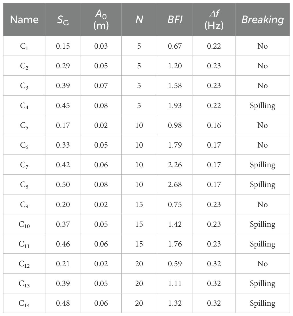
Table 1. Experimental parameters for test cases.

Figure 2 shows the variations of wave surface elevations of the chirped signals for different initial conditions described by Equation 17, the black and red lines represented the wave surface elevations measured at the first and focusing locations. It is evident that the wave shape underwent significant deformation as the wave evolved towards the focusing location. This deformation indicated a pronounced nonlinear evolutionary process. The subsequent analysis in this study focuses on a detailed examination of the nonlinear characteristics and energy transformation of waves as they evolve towards and through the breaking process. It is noteworthy that the primary type of wave breaking observed in the experiment was spilling. The locations of breaking waves were determined based on a combination of observations, experimental records, and data collected from wave gauges. Despite efforts to record wave propagation through videos and deploy multiple recording points, the rapid nature of wave evolution posed challenges in capturing all the breaking locations. Therefore, the recorded breaking instances in the experiment represent only a portion of all the actual occurrences.

Figure 2

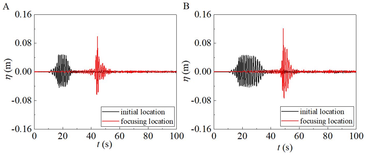
Figure 2. Wave surface elevations for cases C₆ (A) and C₁₃ (B) at initial and focusing locations.

Results

Nonlinear evolutions of spectra

Chirped wave groups deform rapidly, and within a short time and distance, they undergo focusing and subsequent breaking. Figure 3 shows the evolution of the Hilbert spectrum for case C₄, providing an example of capturing rapid nonlinear evolution. In Figure 3, the white solid lines represent the wave surface elevations normalized by the largest crest of the wave surface elevation measured at the first location. The normalized results were then multiplied by a coefficient of 0.6 to facilitate clear visualization of the wave surface elevation and Hilbert spectrum without overlap. The red lines in the subgraph represent the wave surface elevations at the locations where wave breaking occurred. Figure 3C shows that the frequency modulation was significantly enhanced as the wave propagated towards the first breaking point x = 13.9 m, and the wave energy was primarily concentrated in the two waves including the largest wave crest. After the waves break, the energy resided in the largest and previous crests experienced significant dissipation at x = 14.9 m. Simultaneously, there was a noticeable dissipation of high-frequency energy. Comparing Figures 3C, D, it is demonstrated that wave breaking resulted in a notable decrease in energy in the region approximately one wave period preceding the maximum crest A_m. The phenomenon described above effectively demonstrates the primary source and frequency range of energy loss caused by wave breaking. To further confirm and validate whether the source of energy dissipation resulting from wave breaking is approximately one wave ahead of the maximum crest, an analysis of the evolution of energy carried by different waves will be conducted. Figure 4 presents the schematic representation of the wave group segments and the corresponding method of energy representation for each segment. The waves were determined using the peak-to-peak method. The period of the wave preceding the maximum wave peak A_m is denoted as T_p1wave, and by integrating the instantaneous energy IE(t) over T_p1wave, the energy of this wave E_p1wave can be obtained. Similarly, the time duration for the three waves preceding the maximum wave peak is denoted as T_p3wave with the corresponding energy E_p3wave. Similarly, considering the time duration T_6wave for the six waves (including the three waves preceding and following the maximum crest, respectively), the corresponding wave energy E_6wave can be determined.

Figure 3

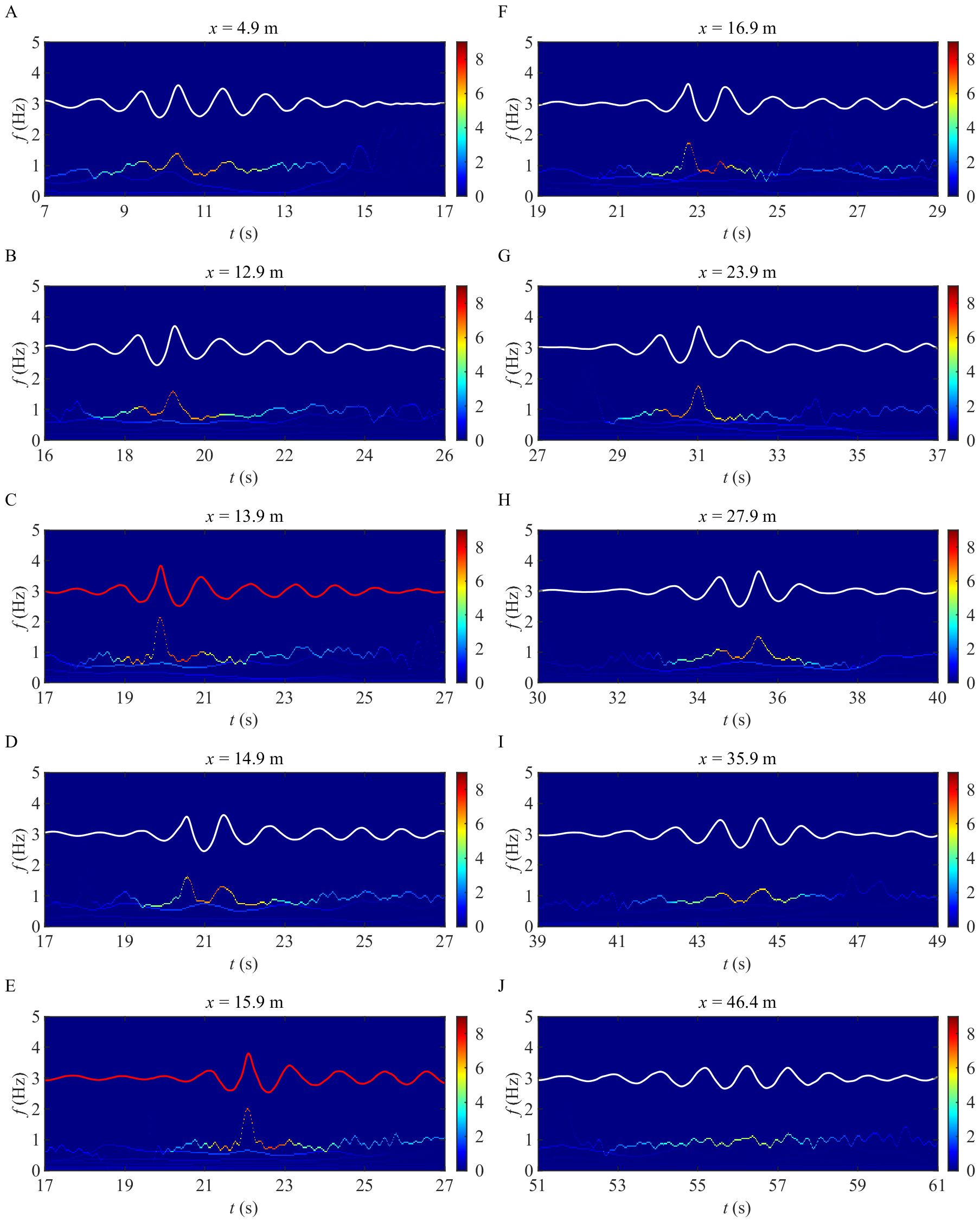
Figure 3. Evolution of Hilbert amplitude spectrum for case C4 at stations (A) x = 4.9 m; (B) x = 12.9 m; (C) x = 13.9 m; (D) x = 14.9 m; (E) x = 15.9 m; (F) x = 16.9 m; (G) x = 23.9 m; (H) x = 27.9 m; (I) x = 35.9 m; (J) x = 46.4 m, the unit of the colorbar is in centimeters. The white solid line in each subplot represents the normalized wave surface elevation. To avoid overlap with the Hilbert spectrum, this normalized wave surface elevation in the figure has been multiplied by a factor of 0.6. The red solid line has the same definition as the white solid line, and the red color is used to signify where the waves reach a local maximum, indicating an imminent breaker.

Figure 4

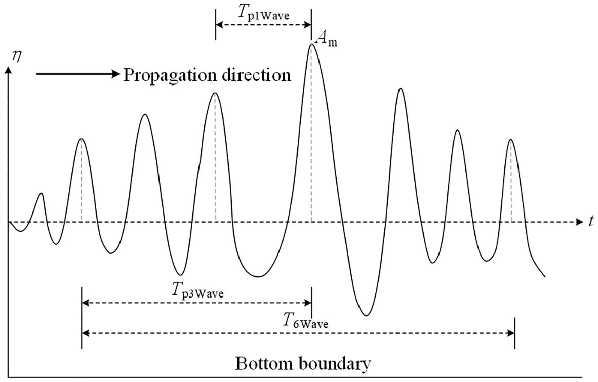
Figure 4. Schematic diagram of the determination method for periods of wave group segments with different numbers of waves.

Figure 5 shows the evolution of the energy carried by wave group segments containing different numbers of waves for the breaking cases. E_T represents the total energy of the entire wave train. The gray area represents the region in which wave breaking occurred. The evolution trends of E_p1Wave and E_p3Wave were approximately identical, and their energies were approximately equivalent. This indicates that among the three waves preceding the maximum crest, the wave directly adjacent to the maximum crest carried most of the energy. This is also well reflected in Figure 6, which represents the spatial evolution of the energy difference between E_p3Wave and E_p1Wave, ΔE_{1_3}. The gray area in Figure 6 represents the breaking region. It is obvious that ΔE_{1_3} approached zero within the breaking region, which further validates the conclusion presented in Figure 5. As shown from Figure 5, as wave evolved, in the breaking region where wave breaking occurred, E_p1Wave showed a behavior of initially increasing and then decreasing. This significant decrease in energy confirms that the energy dissipation caused by breaking occurred primarily in the wave preceding the maximum crest. This confirms the findings depicted in Figure 3 and suggests that there was strong energy focusing on the wavefront during the evolution of waves as they approached breaking. The reason is that the rapid growth in nonlinearity and interaction between waves of different frequencies leads to a rapid concentration of wave energy around the maximum wave. Consequently, the wave group underwent a transformation into a shorter wave group, with energy strongly concentrated (Figure 2).

Figure 5

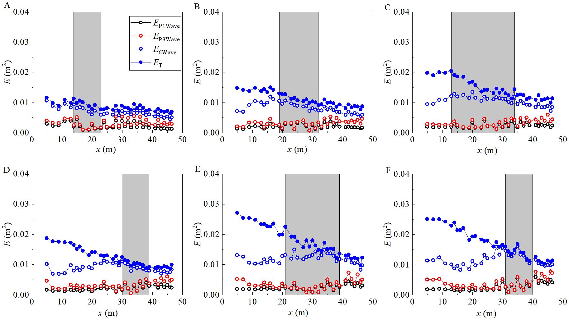
Figure 5. Evolution of the energy of wave group segments containing different numbers of waves for breaking cases (A) C₄, (B) C₇, (C) C₈, (D) C₁₀, (E) C₁₁ and (F) C₁₄. E_p1Wave and E_p3Wave represent the energy carried by the wave group segments consisting of one wave preceding the maximum crest and three waves preceding the maximum crest, respectively; E_6Wave represents the energy carried by the wave group segment consisting of six waves, including the three waves preceding the maximum crest and the three waves following the maximum crest; and E_T represents the total energy of the entire wave group.

Figure 6

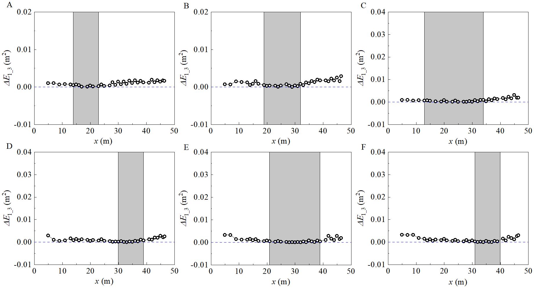
Figure 6. Spatial evolution of the energy difference (ΔE_{1_3}) between E_p3Wave and E_p1Wave for cases (A) C₄, (B) C₇, (C) C₈, (D) C₁₀, (E) C₁₁ and (F) C₁₄. The gray area represents the breaking region.

Additionally, Figure 5 shows that the energy dissipation caused by wave breaking was also evident by observing the evolution of the total energy E. However, it can be observed that for the shorter span of the breaking region, the energy dissipation was mainly concentrated on E_6wave. In contrast, for the wave groups with a longer breaking region span, there was a significant difference between E and E_p6Wave. As waves further evolve, break, and extend beyond the range of the breaking region, this difference gradually decreases until it reaches a state where E and E_p6Wave are approximately equal. This phenomenon is typically associated with cases characterized by a large number of waves and a high degree of modulation instability. This indicates that for longer wave groups, the modulation instability played a more significant role in the generation of large waves. Modulation instability requires a certain distance to develop; thus, in such cases, when the waves are about to break, there is a significant difference between E and E_p6Wave, indicating a relatively uniform distribution of wave group energy and slow energy focusing, which may be due to the insufficient distance for the modulation instability to fully develop. Meanwhile, for the larger number of wave group, although E_p6Wave is derived from waves with higher wave surfaces, comparing with the relatively large number of wave groups, E_p6Wave can only represent a portion of E. This also explain the significant difference between E and E_p6Wave at the beginning of the breaking region. However, as the propagation distance increased, the modulation instability fully developed and became stronger, the wave-group length decreased, and the energy became more concentrated near the maximum wave surface elevation, resulting in a closer relationship between E and E_p6Wave.

Figure 7 presents the time series of the underlying adaptive base functions, IMFs, for case C₄ at the initial and focal locations. Only IMFs up to the fifth order are displayed in Figure 7, because IMFs beyond this order have negligible energy contributions and can be disregarded. The energy evolution of the first five orders of IMFs is depict in Figure 8. It shows that the energy of the first-order IMF IMF₁ is extremely small, it is the white noise content that had not been completely averaged out during the EEMD process. Consequently, IMF₁ is negligible, the subsequent analysis primarily concentrates on examining the evolution of the IMF components from the second to the fifth orders. As shown in Figure 8, the energy of IMF₃ exhibits a consistent decreasing trend throughout its evolution. Even in the case of C₁₃ with higher breaking intensities, IMF₃ maintained a relatively continuous decrease in energy dissipation. This sustained and stable energy dissipation along the propagation direction suggests that the IMF₃ component is a source of non-breaking energy dissipation. In contrast to IMF₃, IMF₂ demonstrates a distinct pattern of initially increasing and then decreasing energy. As a high-order component, IMF₂ follows the following evolutionary trend. Before wave breaking occurs, this component showed an increasing trend. As the wave entered the breaking phase near the end of the breaking region, IMF₂ displayed an overall decreasing trend. However, after the wave evolved beyond the breaking domain, the energy of IMF₂ began to increase. The energy evolution of IMF₂ suggests that energy dissipation during wave breaking primarily originated from the second-order IMF, which represents a short wave group with a relatively higher energy content.

Figure 7

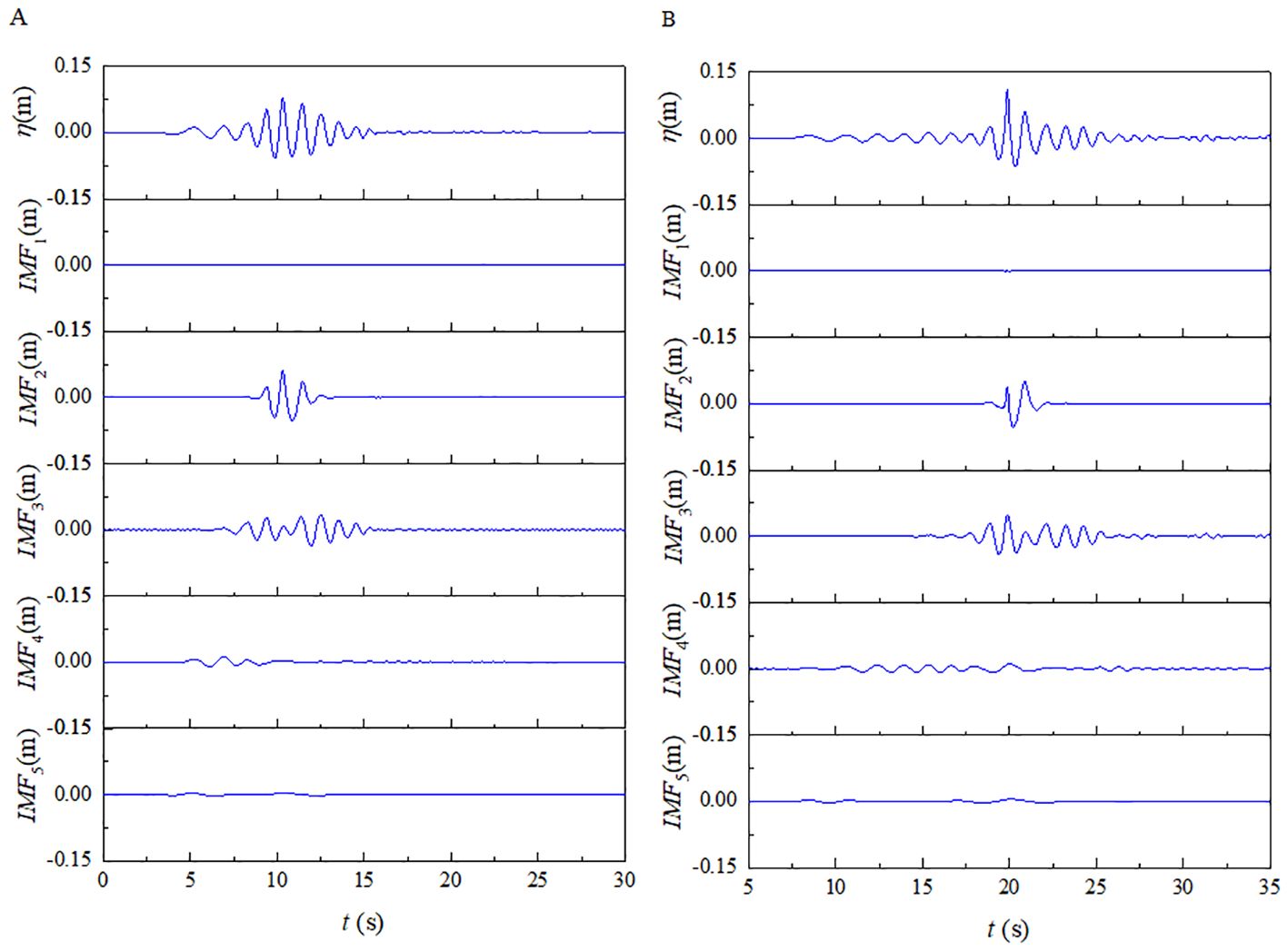
Figure 7. Decomposed results of ensemble empirical mode decomposition for case C₄ at (A) x = 4.9 m and (B) x = 13.9 m.

Figure 8

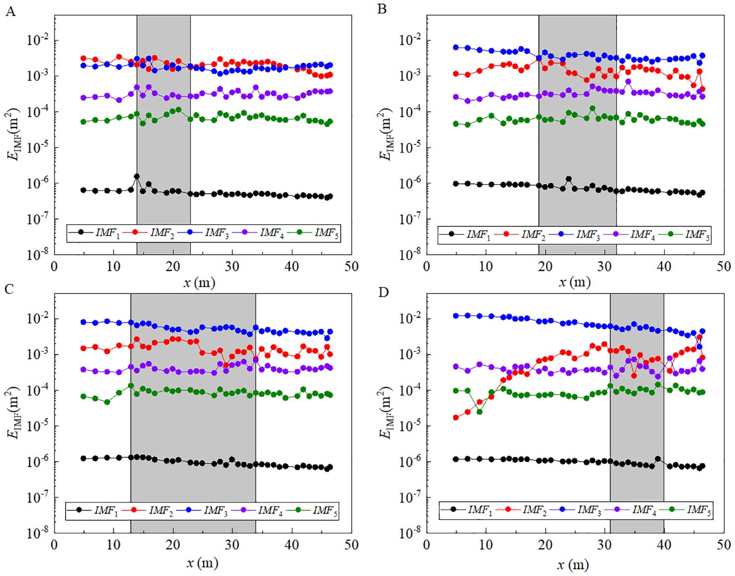
Figure 8. Evolutions of the energy of the top five IMFs for cases (A) C₄, (B) C₇, (C) C₈ and (D) C₁₃. The gray area represents the region of wave breaking.

The lower-frequency components IMF₄ and IMF₅ in Figure 8 exhibited similar evolutionary trends within the breaking zone. They exhibited slight growth with minor fluctuations within the breaking domain, particularly IMF₄, but the magnitude of this growth was relatively small. Throughout the evolutionary process, these components remained almost constant. This phenomenon suggests that the relatively regular lower-frequency components, as observed in Figure 7, maintain relatively stable energy levels. In summary, during the evolution and breaking process of a wave group, most non-breaking and breaking energy dissipations can be attributed to the top two high-frequency components, IMF₃ and IMF₂, respectively. Combining this with results from Figures 3C, D, where high-frequency energy dissipated significantly after the wave breaking, it can be revealed that the high-frequency energy dissipation primarily resulted from the IMF₂, a short wave group. Simultaneously, the low-frequency components maintained nearly constant energy levels.

Figures 3 and 5 clearly depict the regions where significant wave energy dissipation occurred after wave breaking. During the process of waves evolving towards breaking, the frequency components involved in “bound” nonlinear interactions can be identified using wavelet-based bicoherence (Dong et al., 2008b). To illustrate the nonlinear phase coupling action, Figure 9 presents the evolution of the bicoherence for the case depicted in Figure 3. As shown in Figure 9, as the wave evolved towards the focusing point at x = 13.9 m, an increasing number of components were involved in the nonlinear phase coupling, indicating an increase in the energy of the bound waves. After breaking, at x = 14.9 m, it is evident that the energy of the bound waves significantly dissipated, likely owning to wave breaking loss. Furthermore, the corresponding dominant frequency f_p was calculated to be 0.92773 Hz at x = 14.9 m. Notably, the energies of the double, triple and quadruple frequency components dropped sharply to zero. This suggests that the energy residing in these components was released into free waves due to wave breaking. As the waves approached the subsequent position at x = 15.9 m, where the second breaker emerged, the number of wave components engaged in nonlinear bound actions increased. Consequently, the energy associated with the multi-frequency component reappeared. However, following the occurrence of the second breaker, this energy was dissipated albeit to a relatively smaller extent. As the waves evolved beyond the breaking zone (Figure 9H), there was a noticeable decrease in both the number of wave components involved in the nonlinear phase coupling and the energy associated with the bound action. The described evolutionary process illustrates the nonlinear phase coupling is closely related to the energy conversion caused by breaking. When breaking occurs, the disappearance of nonlinear coupling phenomena indicates a decrease in the action of bound waves.

Figure 9

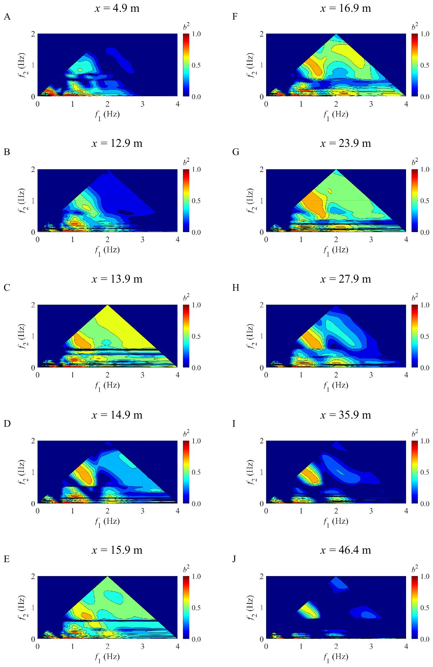
Figure 9. Evolution of wavelet-based bicoherence for case C₄ at stations (A) x = 4.9 m; (B) x = 12.9 m; (C) x = 13.9 m; (D) x = 14.9 m; (E) x = 15.9 m; (F) x = 16.9 m; (G) x = 23.9 m; (H) x = 27.9 m; (I) x = 35.9 m; (J) x = 46.4 m.

Energy transformation analysis

In addition to the nonlinear actions analyzed using the Hilbert spectrum and wavelet-based bicoherence, Fourier energy spectrum is also be incorporated for a comprehensive analysis for the energy variations of wave groups. The variations of the energy spectrum, denoted as ΔS, resulting from wave breaking can be determined as follows. At the identified breaking locations (refer to materials and methods section), if the wave breaks for the first time at position x_b1, the corresponding energy spectrum is S_xb1, the following adjacent measurement point to x_b1 is x_b1 + 1, the corresponding energy spectrum is S_xb1 + 1, and ΔS for the first breaker is the difference between S_xb1 + 1 and S_xb1. Similarly, if the wave breaks for the second time at position x_b2 and the following adjacent measurement point is x_b2 + 1, then ΔS for the second breaker is the difference between S_xb2 + 1 and S_xb2. This pattern continues for subsequent breaking locations. Figure 10 shows the energy variations ΔS induced by the first breaker for cases C₄, C₇, C₈ and C₁₃, the dashed lines denoted the dominant frequencies; to differentiate the dominant frequencies at different measurement points, all dominant frequencies were labeled in the subscript according to the position. As depicted in Figure 10, after wave breaking, the energy associated with components whose frequencies are slightly higher than the initial dominant frequency f_{p, x=4.9m} becomes the main resource of energy loss. Additionally, according to Figure 9, the bound effect significantly decreased after wave breaking. This illustrates that wave breaking can cause significant energy dissipation in slightly higher-frequency bound waves. Simultaneously, regarding the higher-frequency components, there was a visible increase in energy in Figure 10. However, the bound effect for the higher-frequency components diminished significantly after the wave broke in Figure 9. This suggests that the increase in the energy of the higher-frequency components shown in Figure 10 may indicate an enhancement of the free waves derived from the released bound waves and the action of modulation instability.

Figure 10

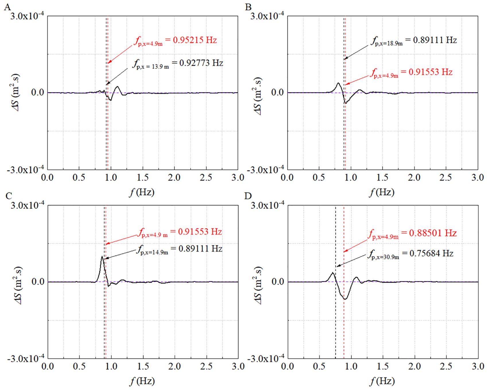
Figure 10. Spectral changes ΔS caused by the first wave breaking for cases (A) C₄, (B) C₇, (C) C₈ and (D) C₁₃. ΔS is determined by calculating the difference between the energy spectra at the position following the breaking location, x_b1 + 1, and the location where the wave broke, x_b1. The red and black dashed lines correspond to the dominant frequencies at the initial measurement point and the locations where the wave group first experiences breaking, respectively.

Under certain wave conditions, multiple instances of wave breaking have been observed along the propagation path. The variations in the energy spectrum ΔS caused by these breakers are depicted in Figure 11, the spectral changes caused by the first, second, and third breakers are represented by black, blue, and dark green solid lines, respectively. It can be found that the first and second breakers caused significant changes in the spectrum. However, there was a significant reduction in the energy changes for the third breaker, as shown in Figures 11A and C. This indicates that the consecutive breakers during the wave propagation process reduced the energy loss of the subsequent breakers. As the number of breakers increased, the impact of the breaker on the energy spectrum gradually diminished. Moreover, Figure 11 indicates that both the lower- and higher-frequency components received significant energy after wave breaking. This can be compared with the substantial decrease in the bound waves in the bicoherence information before and after breaking (Figure 9). It can be inferred that the increase in energy in the high- and low-frequency ranges after breaking does not represent bound-wave energy, but rather free-wave energy (resulting from the enhancement of free waves owning to modulational instability and nonlinear interactions, as well as the release of free waves from bound waves).

Figure 11

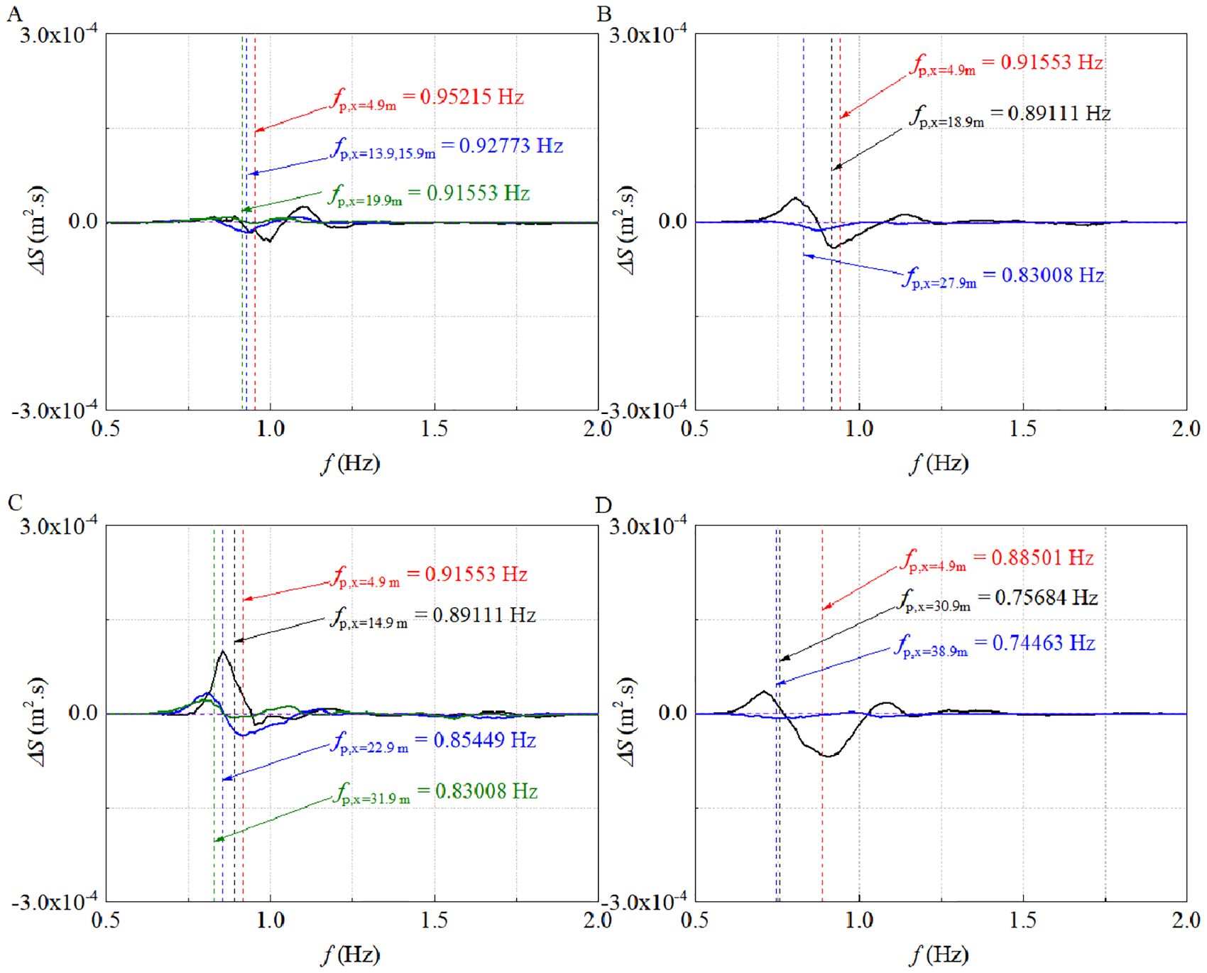
Figure 11. Spectral changes ΔS caused by each identifiable breaking event for cases (A) C₄, (B) C₇, (C) C₈ and (D) C₁₃. The black, blue, and dark green solid lines represent the ΔS caused by the first, second and third breakers, respectively; while the dashed lines corresponding to these colors denote the dominant frequencies at the locations where the first, second and third breakers occurred, respectively. The red dashed lines denote the dominant frequencies at the initial position.

Figure 12 represents the spectral variation between the wave spectra at the focal point, where the wave reached its maximum but did not break, and the initial position, the cases are the same as those in Figure 11. Comparing Figures 11 and 12, it is evident that the magnitude of the non-breaking energy dissipation in the dominant frequency range was considerably higher than the energy dissipation from individual breaking events. Moreover, it was found to be associated with the distance of wave evolution. For instance, in Figures 12A and D, the nonbreaking energy dissipation exhibited a distinct difference owning to the varying focal distances, with the main factor being the close relationship between the frictional energy dissipation and distance. This indicates that non-breaking energy dissipation was mainly contributed by the wave components in the dominant frequency range. In addition to spectral changes, frequency downshift occurred significantly as shown in Figures 10–12. For example, for the breaking events in Figure 11D, the dominant frequency f_p,x=38.9m at the location where the second breaker occurred was 0.74463 Hz, a significant frequency downshift appeared compared with the dominant frequency at the initial location (f_p,x=4.9m = 0.88501 Hz). In Figure 12, all the cases were non-breaking, but the results show that the frequency shift occurred for them, suggesting that wave breaking was not the sole determinant of the frequency downshift.

Figure 12

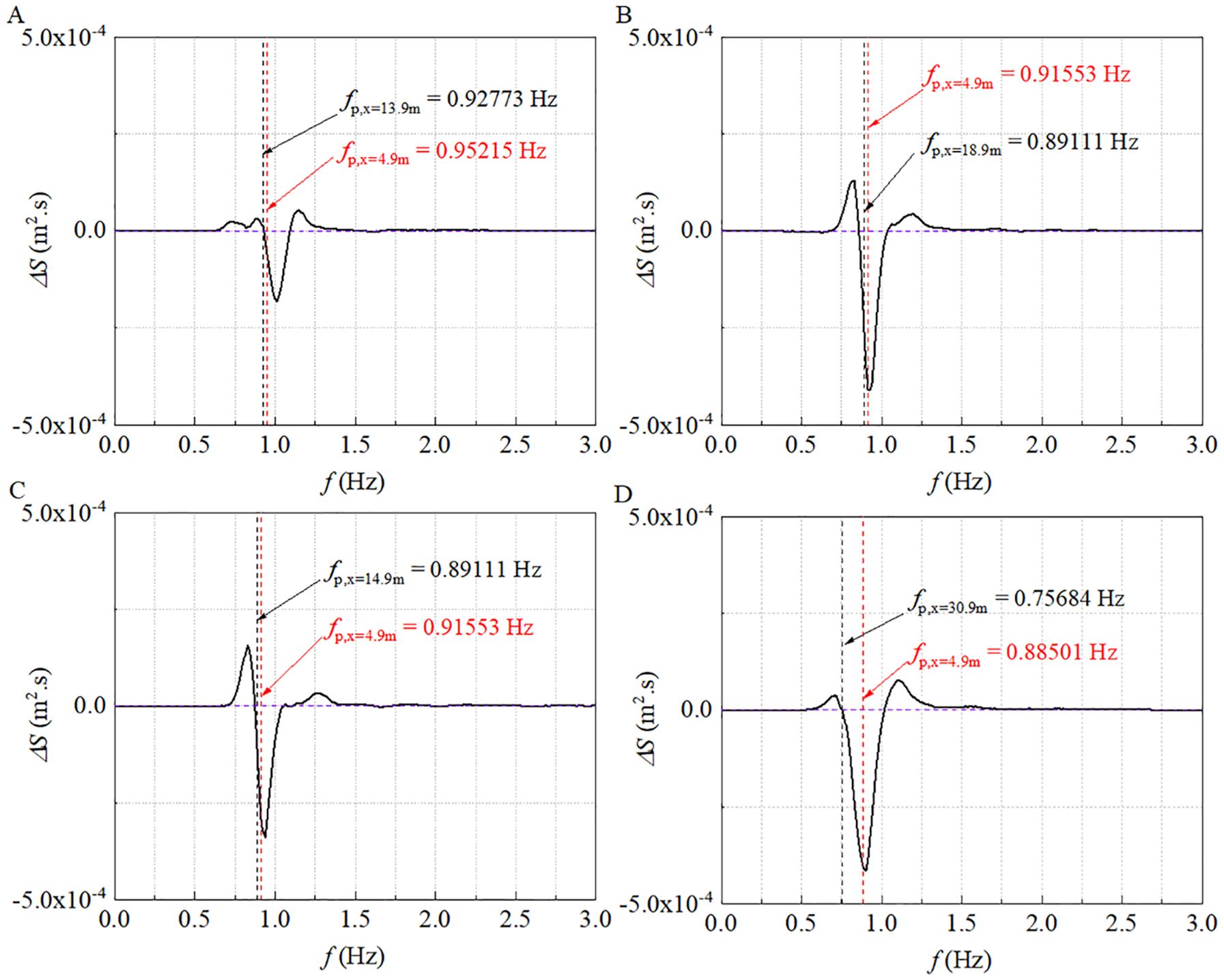
Figure 12. Spectral changes ΔS caused by non-breaking factors for cases (A) C₄, (B) C₇, (C) C₈ and (D) C₁₃. ΔS is derived from the difference between the energy spectra at the location where the wave reached the maximum and the initial measurement point, the region after wave breaking is not included.

Energy dissipation rate

To differentiate between non-breaking and breaking energy dissipation, the total energy at each measurement point was calculated to provide an overview of the energy evolution along the wave propagation.

According to Tian et al. (2010), the energy decay caused by viscosity follows an exponential decay rate:

$\begin{array}{ll}{E}_{fitting}=E_{first}{e}^{-\sigma x},& (18)\end{array}$

where E_fitting is the fitting curve for the total energy obtained through fitting using the least squares method; E_first is the initial value for the fitting curve of energy; and the parameter σ represents the energy decay rate caused by factors such as the viscosity of the water, boundary layers, sidewalls, and bottom of the water tank. In the experiment, the parameter σ was approximately O(0.01), as derived from the fitting results for the non-breaking cases shown in Table 2. Once the parameter σ was determined, the energy loss rate caused by non-breaking and breaking waves was calculated using the same method as described by Tian et al. (2010).

Table 2

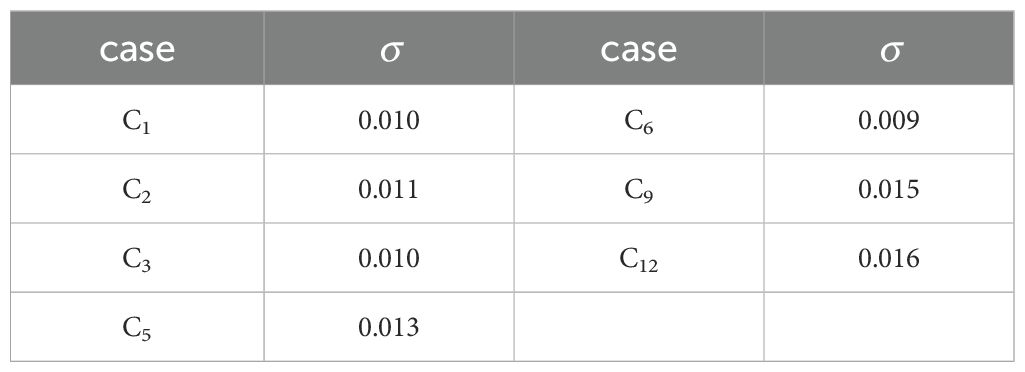
Table 2. Exponential energy decay rate along propagation caused by non-breaking factors.

Figure 13 illustrates the total energy evolution along the water channel for the two non-breaking and two breaking cases, the black dashed lines are the fitted curves. In the non-breaking cases, the difference between the initial and final values of the fitted curve is regarded as non-breaking viscous dissipation. The ratio of this dissipation to the initial value of the energy-fitted curve was considered the non-breaking energy dissipation rate. For the breaking wave groups, measurements upstream and downstream of wave breaking are individually fitted with the energy decay rate of the non-breaking case to account for the non-breaking dissipation. Subsequently, the altitude intercept ΔE between the fitting curves of the upstream and downstream of the breaking zone was considered as the energy dissipation caused by wave breaking. To determine the position at which the wave started to break, it was placed upstream on the energy-fitted curve. The value of the fitted curve at this position was regarded as the initial energy of the breaking zone, denoted as E₀. The section indicated by vertical dashed lines in Figure 13 corresponds to the breaking zone.

Figure 13

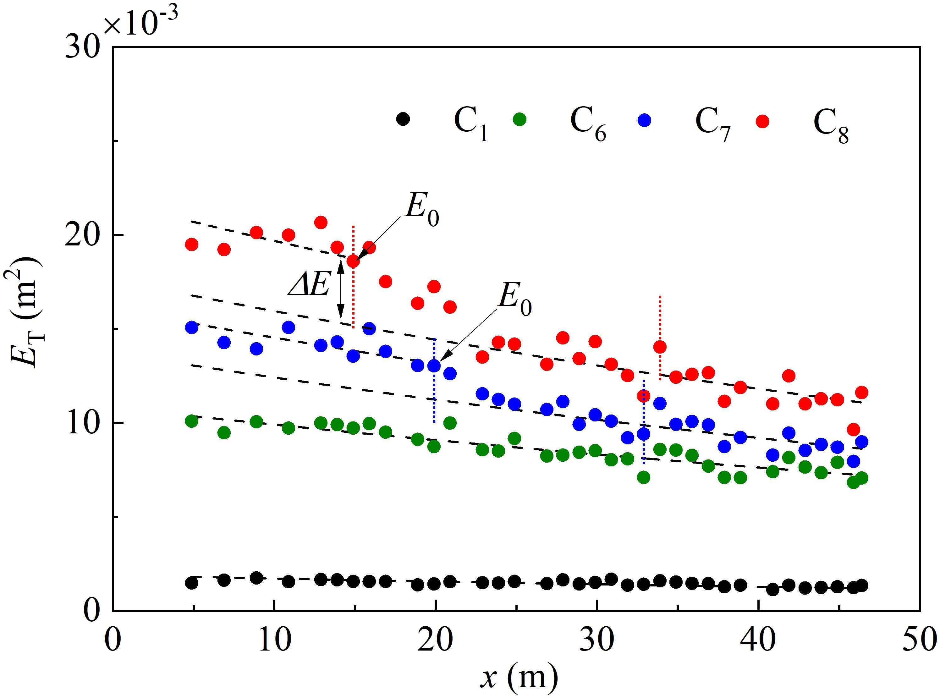
Figure 13. Estimation of energy dissipation due to non-breaking viscosity and wave breaking, shown for cases C₁, C₆, C₇ and C₈. The thick dashed lines are the fitting curves; the vertical short-dot lines denote the start and end thresholds for breaking length scale. Non-breaking losses are estimated from the exponential fit of the non-breaking wave measurements. For the breaking cases, based on the exponential fit, E₀ is the estimated energy just prior to wave breaking, and the difference between the exponential fit for upstream and downstream measurements at the location of breaking onset is denoted ΔE, which is estimated as the energy dissipation caused by wave breaking.

Table 3 presents the energy dissipation rates caused by non-breaking factors, such as viscosity, alongside those for by wave breaking. The nonbreaking energy dissipation rates exceeded 30%, with a mean dissipation rate of 39%. This indicates that the energy loss resulting from viscosity accounted for approximately 40% of the initial energy over a propagation distance of approximately 30 wavelengths. The energy dissipation caused by wave breaking cases in the experiment is listed in the right column of Table 3. The results illustrate the influence of the initial conditions on the wave breaking. For a smaller initial number of waves, such as in case C₄, the energy dissipation caused by the wave breaking was relatively small. However, as the number of waves increased, the rate of energy dissipation owning to wave breaking was approximately 20%. This indicates a potential link between the number of carrier waves and wave breaking phenomena.

Table 3

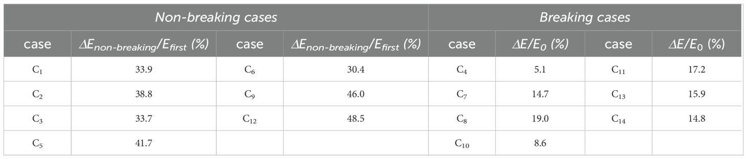
Table 3. Energy dissipation rates caused by non-breaking factors such as viscosity and caused by wave breaking, respectively.

Figure 14A represents the relationship between the number of carrier waves N and the maximum wave surface elevation A_m. The maximum wave surface elevation exhibited a substantial increase as the number of waves increased. This implies that wave groups with a larger number of carrier waves had a higher propensity to generate extreme waves with larger amplitudes. Notably, there was a substantial increase in the maximum crest amplitude for cases within the shaded region in Figure 14A compared to the other values. Furthermore, the BFI values of these cases in the shaded region were consistently greater than 1 (Figure 14C). This observation implies that the presence of modulation instability induced nonlinear amplification within these wave groups, resulting in significant wave surface elevation. Moreover, the length of the wave tank in this experiment allowed the modulation instability to develop significantly. Consequently, with the combined influence of dispersion focusing and modulation instability, the nonlinearity of the waves progressively intensified. As the modulation instability progressed, the distance at which the maximum wave surface elevation occurred gradually increased. It can also be inferred that Once BFI exceeded its critical threshold, wave groups carrying multiple carrier waves exhibited extreme waves at longer distances, which subsequently led to wave breaking, as illustrated in Figure 14B.

Figure 14

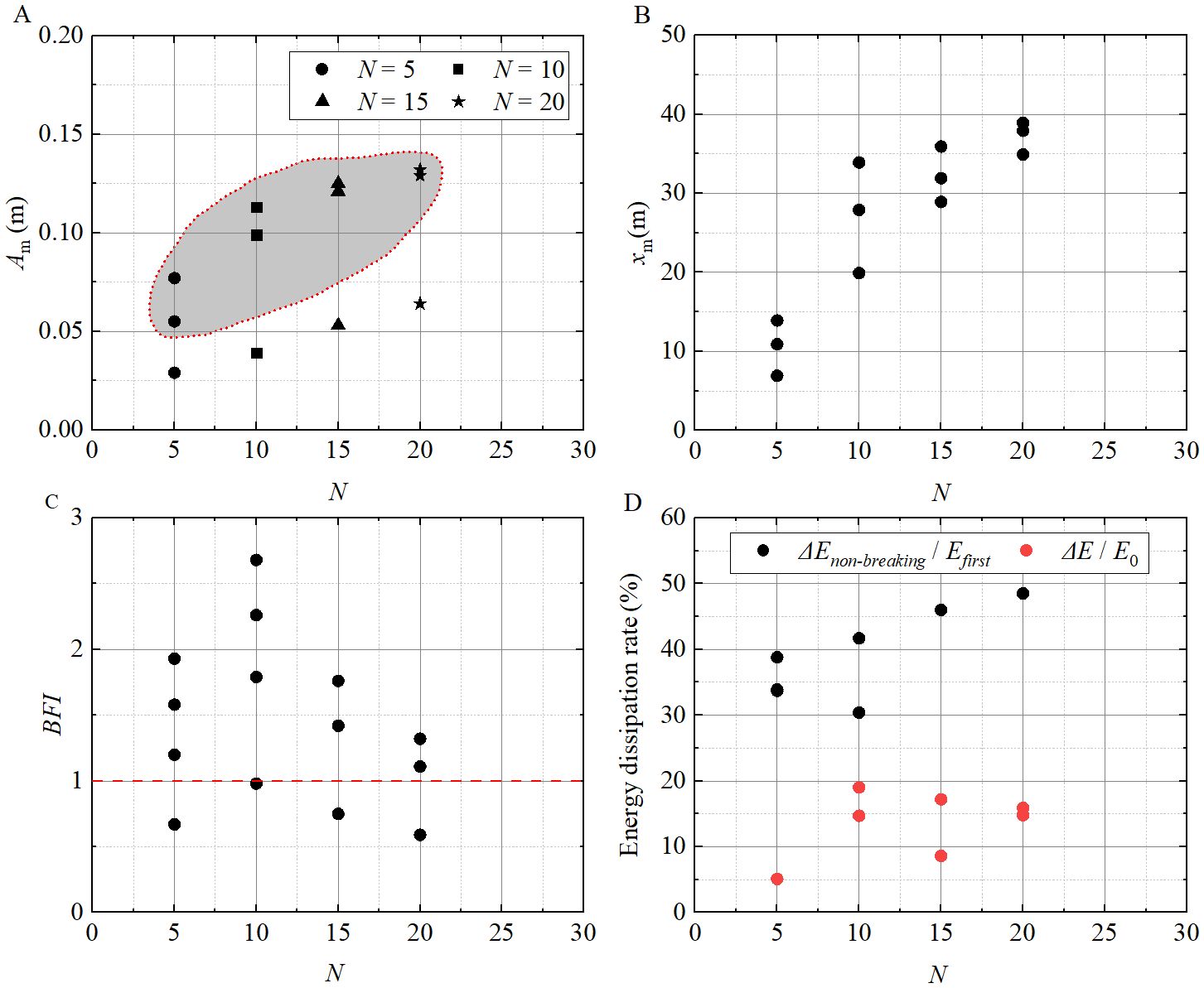
Figure 14. The relationship between the number of carrier waves N and the maximum wave surface elevation A_m (A), the location where the maximum wave surface elevation occurred, x_m (B), the BFI (C), and the energy dissipation rate (D).

The above analysis elucidates the strong correlation between the number of carrier waves in a wave group and the characteristics of wave breaking. Additionally, Figure 14D provides insight into the relationship between the number of carrier waves and energy dissipation rate. When the number of carrier waves increased, both the nonbreaking and breaking energy dissipation rates exhibited an overall increasing trend. The amount of nonbreaking energy dissipation rate was generally more than twice the breaking energy dissipation rate. The maximum wave surface elevations of wave groups with a greater number of carrier waves occurred at greater distances (Figures 14A, B), resulting in relatively higher non-breaking energy dissipation. Figure 14D also provides a preliminary increasing dependency between the number of carrier waves and the breaking energy dissipation rate. Due to the complexity of the breaking process, the simplification in obtaining breaking energy in the preliminary analysis may lead to differences between the estimated and actual energy, thus affecting this dependency. Therefore, Subsequent investigations will be conducted to further explore this relationship and to provide a more comprehensive analysis.

Additionally, according to Tables 1 and 3, for cases with the same number of waves, the wave steepness was correlated with the energy dissipation rate caused by wave breaking. Furthermore, as the number of waves and wave steepness increased, the intensity, frequency, and duration of wave-breaking events during the evolution of wave groups were affected. Overall, the confluence of amplified wave amplitudes, intensified nonlinear effects, and the propensity for wave breaking rendered wave groups with a greater number of carrier waves more susceptible to the emergence of larger, extreme waves and subsequent wave breaking.

Discussion and conclusion

The aim of the study was to analyze the energy variations and nonlinear characteristics of wave groups with different initial conditions. The evolution of the Hilbert energy spectra provides insights into the energy loss caused by wave breaking, mainly originating from high-frequency content, whether initial or subsequent breaking. Taking case C₄ as an example (Figure 3), when the wave was about to break for the first time at x = 13.9 m, the first-order instantaneous frequency reached 2.17 Hz. However, after breaking occurred at x = 14.9 m, the maximum instantaneous frequency dropped to 1.63 Hz. This signifies a significant loss of energy in the high-frequency components due to the breaking process. The analysis of wavelet bicoherence further confirmed that the bound effect significantly decreased after wave breaking (Figure 9). Therefore, the findings from both methods indicate a close relationship between the modulation of the instantaneous frequency and the bound effect. These findings align with those of a study conducted by He et al. (2023b) on the behavior of random waves under varying water depths. However, analysis of the energy spectra (Figures 10, 11) before and after breaking revealed minimal changes in the energy above 1.25 Hz, most energy changes were concentrated in the dominant frequency region, resulting in a wider frequency bandwidth. This indicates a significant shift in energy towards the free-wave energy in the dominant frequency region of the energy spectrum. However, it remains challenging to determine whether this energy change primarily stems from the modulation instability or from the release of free waves after breaking. Consequently, further in-depth research is necessary to investigate the fundamental processes involved in the energy transformation of wave components during breaking.

Based on the energy analysis of the wave evolution and wave breaking, the following key conclusions can be drawn:

1. After the wave breaking, a distinct portion was identified by the Hilbert spectrum in the time series of the wave surface, which experienced a noticeable energy loss. This section persisted for approximately one wave period, whereas other segments exhibited minor energy fluctuations.

2. Following wave breaking, there was a noticeable dissipation of high-frequency energy, particularly above the dominant frequency range. Moreover, the energy of the bound waves exhibited a noticeable decrease, although the magnitude of this change was relatively small compared to the energy in the dominant frequency region. This indicates that, under the conditions of modulation instability, the dissipation of energy resulting from wave breaking in finite water depths primarily manifested as the conversion of energy into free waves derived from both the released bound waves and the action of modulation instability.

3. As the wave evolved, the energy of the main intrinsic mode functions exhibited a distinct variation. For a component that presented itself as a short wave group with significant energy, the energy increased consistently and then decreased when the wave began to break. Therefore, this underlying component accounted for the main energy dissipation caused by wave breaking.

4. This study examined the energy loss associated with the non-breaking and breaking factors. For the non-breaking cases, the mean energy-loss rate was approximately 40%. However, for breaking cases, the energy loss rate caused by wave breaking exhibited a wide range: wave groups with fewer waves experienced relatively lower energy dissipation rate; conversely, wave groups with a larger number of waves exhibited relatively higher energy dissipation.

Data availability statement

The raw data supporting the conclusions of this article will be made available by the authors, without undue reservation.

Author contributions

GW: Funding acquisition, Writing – review & editing. YH: Writing – original draft, Writing – review & editing, Methodology. YZ: Visualization, Writing – review & editing. JL: Conceptualization, Writing – review & editing. HM: Methodology, Writing – review & editing.

Funding

The author(s) declare that financial support was received for the research, authorship, and/or publication of this article. This work was financially supported by program for scientific research start-upfunds of Guangdong Ocean University (grant number R20068, R20069); the Guangdong Basic and Applied Basic Research Foundation (grant number 2024A1515012321, 2023A1515010890, 2022A1515240039); the Zhanjiang City Science and Technology Plan Project (grant number 2021B01416); the Open Fund of State Key Laboratory of Coastal and Offshore Engineering, Dalian University of Technology (grant number LP2403); the Ocean Youth Talent Project of Zhanjiang Science and Technology Bureau (grant number 2021E05010); the Special Fund Competition Allocation Project of Guangdong Science and Technology Innovation Strategy (grant number 2023A01022); and the National Natural Science Foundation of China (grant number 52001071); 2023 Guangdong Ocean University Undergraduate Innovation and Entrepreneurship Training Program Project (grant number 010403072312).

Acknowledgments

The authors express gratitude to the reviewers for their valuable comments and suggestions.

Conflict of interest

The authors declare that the research was conducted in the absence of any commercial or financial relationships that could be construed as a potential conflict of interest.

Publisher’s note

All claims expressed in this article are solely those of the authors and do not necessarily represent those of their affiliated organizations, or those of the publisher, the editors and the reviewers. Any product that may be evaluated in this article, or claim that may be made by its manufacturer, is not guaranteed or endorsed by the publisher.

References

Abroug I., Abcha N., Jarno A., Marin F. (2020). Laboratory study of non-linear wave–wave interactions of extreme focused waves in the nearshore zone. Natural Hazards Earth System Sci. 20, 3279–3291. doi: 10.5194/nhess-20-3279-2020

Crossref Full Text | Google Scholar

Babanin A. V., Young I. R., Banner M. L. (2001). Breaking probabilities for dominant surface waves on water of finite constant depth. J. Geophysical Res. 106, 11659–11676. doi: 10.1029/2000JC000215

Crossref Full Text | Google Scholar

Banner M. L., Peirson W. L. (2007). Wave breaking onset and strength for two-dimensional deep-water wave groups. J. Fluid Mechanics 585, 93–115. doi: 10.1017/S0022112007006568

Crossref Full Text | Google Scholar

Buldakov E., Stagonas D., Simons R. (2017). Extreme wave groups in a wave flume: Controlled generation and breaking onset. Coast. Eng. 128, 75–83. doi: 10.1016/j.coastaleng.2017.08.003

Crossref Full Text | Google Scholar

Chen H. F., Zou Q. P. (2017). Wind and current effects on extreme wave formation and breaking. J. Phys. Oceanography 47, 1817–1841. doi: 10.1175/JPO-D-16-0183.1

Crossref Full Text | Google Scholar

Chen H. Z., Tang X. C., Zhang R., Gao J. L. (2018). Effect of bottom slope on the nonlinear triad interactions in shallow water. Ocean Dynamics 68, 469–483. doi: 10.1007/s10236-018-1143-y

Crossref Full Text | Google Scholar

Chen H. Z., Zhao Y. S., Mei L. L., Gui F. K. (2024). Laboratory observation of nonlinear wave shapes due to spatial varying opposing currents. Coast. Eng. 190, 104500. doi: 10.1016/j.coastaleng.2024.104500

Crossref Full Text | Google Scholar

Dong G. H., Gao X., Ma X. Z., Ma Y. X. (2020). Energy properties of regular water waves over horizontal bottom with increasing nonlinearity. Ocean Eng. 218, 108159. doi: 10.1016/j.oceaneng.2020.108159

Crossref Full Text | Google Scholar

Dong G. H., Ma Y. X., Ma X. Z. (2008a). Cross-shore variations of wave groupiness by wavelet transform. Ocean Eng. 35, 676–684. doi: 10.1016/j.oceaneng.2007.12.004

Crossref Full Text | Google Scholar

Dong G. H., Ma Y. X., Ma X. Z., Perlin M., Yu B., Xu J. W. (2008b). Experimental study of wave-wave nonlinear interactions using the wavelet-based bicoherence. Coast. Eng. 55, 741–752. doi: 10.1016/j.coastaleng.2008.02.015

Crossref Full Text | Google Scholar

Fu R. L., Ma Y. X., Dong G. H., Perlin M. (2021). A wavelet-based wave group detector and predictor of extreme events over unidirectional sloping bathymetry. Ocean Eng. 229, 108936. doi: 10.1016/j.oceaneng.2021.108936

Crossref Full Text | Google Scholar

Fu R. L., Ma Y. X., Dong G. H., Perlin M. (2022). A new predictor of extreme events in irregular waves considering interactions of adjacent wave groups. Ocean Eng. 244, 110441. doi: 10.1016/j.oceaneng.2021.110441

Crossref Full Text | Google Scholar

Gao J. L., Ma X. Z., Dong G. H., Chen H. Z., Liu Q., Zang J. (2021). Investigation on the effects of Bragg reflection on harbor oscillations. Coast. Eng. 170, 103977. doi: 10.1016/j.coastaleng.2021.103977

Crossref Full Text | Google Scholar

Gao J. L., Hou L. H., Liu Y. Y., Shi H. B.. (2024a). Influences of Bragg reflection on harbor resonance triggered by irregular wave groups. Ocean Engineering. 305, 117941.

Google Scholar

Gao J. L., Mi C. L., Song Z. W., Liu Y. Y. (2024b). Transient gap resonance between two closely-spaced boxes triggered by nonlinear focused wave groups. Ocean Eng. 305, 117938. doi: 10.1016/j.oceaneng.2024.117938

Crossref Full Text | Google Scholar

Gao J. L., Shi H. B., Zang J., Liu Y. Y. (2023). Mechanism analysis on the mitigation of harbor resonance by periodic undulating topography. Ocean Eng. 281, 114923. doi: 10.1016/j.oceaneng.2023.114923

Crossref Full Text | Google Scholar

Gibson R. S., Swan C. (2007). The evolution of large ocean waves: the role of local and rapid spectral changes. Proc. R. Soc. A: Mathematical Phys. Eng. Sci. 463, 21–48. doi: 10.1098/rspa.2006.1729

Crossref Full Text | Google Scholar

He Y. L., Chen H. Z., Yang H., He D. B., Dong G. H. (2023a). Experimental investigation on the hydrodynamic characteristics of extreme wave groups over unidirectional sloping bathymetry. Ocean Eng. 114982, 1–16. doi: 10.1016/j.oceaneng.2023.114982

Crossref Full Text | Google Scholar

He Y. L., Ma Y. X., Mao H. F., Dong G. H., Ma X. Z. (2022). Predicting the breaking onset of wave groups in finite water depths based on the Hilbert-Huang transform method. Ocean Eng. 247, 110733. doi: 10.1016/j.oceaneng.2022.110733

Crossref Full Text | Google Scholar

He Y. L., Wu G. L., Mao H. F., Chen H. Z., Lin J. B., Dong G. H. (2023b). An experimental study on nonlinear wave dynamics for freak waves over an uneven bottom. Front. Mar. Sci. 10, 1150896. doi: 10.3389/fmars.2023.1150896

Crossref Full Text | Google Scholar

Holthuijsen L. H., Herbers T. H. C. (1986). Statistics of breaking waves observed as whitecaps in the open sea. J. Phys. Oceanography 16, 290–297. doi: 10.1175/1520-0485(1986)016<0290:SOBWOA>2.0.CO;2

Crossref Full Text | Google Scholar

Huang N. E., Shen Z., Long S. R., Wu M. C., Shih H. H., Zheng Q., et al. (1998). The empirical mode decomposition and the Hilbert spectrum for nonlinear and non-stationary time series analysis. Proc. R. Soc. A: Mathematical Phys. Eng. Sci. 454, 903–995. doi: 10.1098/rspa.1998.0193

Crossref Full Text | Google Scholar

Liang S. X., Zhang Y. H., Sun Z. C., Chang Y. L. (2017). Laboratory study on the evolution of waves parameters due to wave breaking in deep water. Wave Motion 68, 31–42. doi: 10.1016/j.wavemoti.2016.08.010

Crossref Full Text | Google Scholar

Luo M., Rubinato M., Wang X., Zhao X. Z. (2022). Experimental investigation of freak wave actions on a floating platform and effects of the air gap. Ocean Eng. 253, 111192. doi: 10.1016/j.oceaneng.2022.111192

Crossref Full Text | Google Scholar

Ma Y. X., Chen H. Z., Ma X. Z., Dong G. H. (2017). A numerical investigation on nonlinear transformation of obliquely incident random waves on plane sloping bottoms. Coast. Eng. 130, 65–84. doi: 10.1016/j.coastaleng.2017.10.003

Crossref Full Text | Google Scholar

Ma Y. X., Dong G. H., Perlin M., Ma X. Z., Wang G. (2012). Experimental investigation on the evolution of the modulation instability with dissipation. J. Fluid Mechanics 711, 101–121. doi: 10.1017/jfm.2012.372

Crossref Full Text | Google Scholar

Ma Y. X., Yuan C. F., Ai C. F., Dong G. H. (2020). Reconstruction and analysis of freak waves generated from unidirectional random waves. J. Offshore Mechanics Arctic Eng. 142, 041201–041215. doi: 10.1115/1.4045766

Crossref Full Text | Google Scholar

Mahmoudof S. M., Badiei P., Siadatmousavi S. M., Chegini V. (2016). Observing and estimating of intensive triad interaction occurrence in very shallow water. Continental Shelf Res. 122, 68–76. doi: 10.1016/j.csr.2016.04.003

Crossref Full Text | Google Scholar

Mahmoudof S. M., Hajivalie F. (2021). Experimental study of hydraulic response of smooth submerged breakwaters to irregular waves. Oceanologia 63, 448–462. doi: 10.1016/j.oceano.2021.05.002

Crossref Full Text | Google Scholar

Malila M. P., Thomson J., Breivik Ø., Benetazzo A., Scanlon B., Ward B. (2022). On the groupiness and intermittency of oceanic whitecaps. J. Geophysical Research: Oceans 127, e2021JC017938. doi: 10.011029/012021JC017938

Crossref Full Text | Google Scholar

Onorato M., Osborne A. R., Serio M., Cavaleri L., Brandini C., Stansberg C. T. (2006). Extreme waves, modulational instability and second order theory: wave flume experiments on irregular waves. Eur. J. Mechanics - B/Fluids 25, 586–601. doi: 10.1016/j.euromechflu.2006.01.002

Crossref Full Text | Google Scholar

Onuki Y., Hibiya T. (2019). Parametric subharmonic instability in a narrow-band wave spectrum. J. Fluid Mechanics 865, 247–280. doi: 10.1017/jfm.2019.44

Crossref Full Text | Google Scholar

Peregrine D. H. (1976). Interaction of Water Waves and Currents. 9–117.

Google Scholar

Porubov A. V., Tsuji H., Lavrenov I. V., Oikawa M. (2005). Formation of the rogue wave due to non-linear two-dimensional waves interaction. Wave Motion 42, 202–210. doi: 10.1016/j.wavemoti.2005.02.001

Crossref Full Text | Google Scholar

Rapp R. J., Melville W. K. (1990). Laboratory measurements of deep-water breaking waves. Philos. Trans. R. Soc. London. Ser. A Mathematical Phys. Eng. Sci. 331, 735–800. doi: 10.1098/rsta.1990.0098

Crossref Full Text | Google Scholar

Shemer L., Goulitski K., Kit E. (2007). Evolution of wide-spectrum unidirectional wave groups in a tank: an experimental and numerical study. Eur. J. Mechanics-B/Fluids 26, 193–219. doi: 10.1016/j.euromechflu.2006.06.004

Crossref Full Text | Google Scholar

Song J. B., Banner M. L. (2002). On determining the onset and strength of breaking for deep water waves. Part I: unforced irrotational wave groups. J. Phys. Oceanography 32, 2541–2558. doi: 10.1175/1520-0485-32.9.2541

Crossref Full Text | Google Scholar

Tian Z. G., Perlin M., Choi W. Y. (2010). Energy dissipation in two-dimensional unsteady plunging breakers and an eddy viscosity model. J. Fluid Mechanics 655, 217–257. doi: 10.1017/S0022112010000832

Crossref Full Text | Google Scholar

Toffoli A., Bitner-Gregersen E. M., Osborne A. R., Serio M., Monbaliu J., Onorato M. (2011). Extreme waves in random crossing seas: Laboratory experiments and numerical simulations. Geophysical Res. Lett. 38, L06605. doi: 10.1029/2011GL046827

Crossref Full Text | Google Scholar

Trulsen K., Raustøl A., Jorde S., Rye L. (2020). Extreme wave statistics of long-crested irregular waves over a shoal. J. Fluid Mechanics 882, R2, 1–11. doi: 10.1017/jfm.2019.861

Crossref Full Text | Google Scholar

Trulsen K., Zeng H., Gramstad O. (2012). Laboratory evidence of freak waves provoked by non-uniform bathymetry. Phys. Fluids 24, 740–310. doi: 10.1063/1.4748346

Crossref Full Text | Google Scholar

Veltcheva A., Guedes Soares C. (2015). Wavelet analysis of non-stationary sea waves during Hurricane Camille. Ocean Eng. 95, 166–174. doi: 10.1016/j.oceaneng.2014.11.035

Crossref Full Text | Google Scholar

Veltcheva A. D., Guedes Soares C. (2016). Analysis of wave groups by wave envelope-phase and the Hilbert Huang transform methods. Appl. Ocean Res. 60, 176–184. doi: 10.1016/j.apor.2016.09.006

Crossref Full Text | Google Scholar

Veltcheva A., Soares C. G. (2016). Nonlinearity of abnormal waves by the Hilbert–Huang Transform method. Ocean Eng. 115, 30–38. doi: 10.1016/j.oceaneng.2016.01.031

Crossref Full Text | Google Scholar

Viotti C., Dias F. (2014). Extreme waves induced by strong depth transitions: Fully nonlinear results. Phys. Fluids 26, 051705. doi: 10.1063/1.4880659

Crossref Full Text | Google Scholar

Wang L., Li J. X., Liu S. X., Fan Y. P. (2020). Experimental and numerical studies on the focused waves generated by double wave groups. Front. Energy Res. 8. doi: 10.3389/fenrg.2020.00133

PubMed Abstract | Crossref Full Text | Google Scholar

Wang G., Yu Y., Tao A. F., Zheng J. H. (2022). An analytic investigation of primary and cross waves in the flume with a shoal. Ocean Eng. 244, 110428. doi: 10.1016/j.oceaneng.2021.110428

Crossref Full Text | Google Scholar

Wu Z. H., Huang N. E. (2008). Ensemble empirical mode decomposition: a noise assisted data analysis method. Adv. Adaptive Data Anal. 1, 1–41. doi: 10.1142/S1793536909000047

Crossref Full Text | Google Scholar

Wu C. H., Yao A.F. (2004). Laboratory measurements of limiting freak waves on currents. J. Geophysical Res. 109, C12002. doi: 10.1029/2004JC002612

Crossref Full Text | Google Scholar

Zhang R., Ahammad N. A., Raju C. S. K., Upadhya S. M., Shah N. A., Yook S.-J. (2022b). Quadratic and linear radiation impact on 3D convective hybrid nanofluid flow in a suspension of different temperature of waters: Transpiration and Fourier Fluxes. Int. Commun. Heat Mass Transfer 138, 106418. doi: 10.1016/j.icheatmasstransfer.2022.106418

Crossref Full Text | Google Scholar

Zhang J., Benoit M. (2021). Wave–bottom interaction and extreme wave statistics due to shoaling and de-shoaling of irregular long-crested wave trains over steep seabed changes. J. Fluid Mechanics 912, A28. doi: 10.1017/jfm.2020.1125

Crossref Full Text | Google Scholar

Zhang J., Benoit M., Ma Y. X. (2022a). Equilibration process of out-of-equilibrium sea-states induced by strong depth variation Evolution of coastal wave spectrum and representative parameters. Coast. Eng. 174, 104099. doi: 10.1016/j.coastaleng.2022.104099

Crossref Full Text | Google Scholar

Zhao X. Z., Sun Z. C. (2010). Influence of wave breaking on wave statistics for finite-depth random wave trains. J. Mar. Sci. Appl. 9, 8–13. doi: 10.1007/s11804-010-9012-1

Crossref Full Text | Google Scholar

Zhou B. Z., Ding K. L. X., Wang J. H., Wang L., Jin P., Tang T. N. (2023). Experimental study on the interactions between wave group in double-wave-group focusing. Phys. Fluids 35, 037118. doi: 10.1063/5.0142042

Crossref Full Text | Google Scholar