 Chunyong Ma
 Qianqian Hou
 Chen Liu
 Yalong Liu
 Yingying Duan
 Chengfeng Zhang
 Ge Chen
95% of researchers rate our articles as excellent or good
Learn more about the work of our research integrity team to safeguard the quality of each article we publish.
Find out more
ORIGINAL RESEARCH article
Front. Mar. Sci. , 03 September 2024
Sec. Ocean Observation
Volume 11 - 2024 | https://doi.org/10.3389/fmars.2024.1432770
Sea state bias (SSB) is a crucial error of satellite radar altimetry over the ocean surface. For operational nonparametric SSB (NPSSB) models, such as two-dimensional (2D) or three-dimensional (3D) NPSSB, the solution process becomes increasingly complex and the construction of their regression functions pose challenges as the dimensionality of relevant variables increases. And most current SSB correction models for altimeters still follow those of traditional nadir radar altimeters, which limits their applicability to Synthetic Aperture Radar altimeters. Therefore, to improve this situation, this study has explored the influence of multi-dimensional SSB models on Synthetic Aperture Radar altimeters. This paper proposes a deep learning-based SSB estimation model called SNSSB, which employs a Siamese network framework, takes various multi-dimensional variables related to sea state as inputs, and uses the difference in sea surface height (SSH) at self-crossover points as the label. Experiments were conducted using Sentinel-6 self-crossover data from 2021 to 2023, and the model is evaluated using three main metrics: the variance of the SSH difference, the explained variance, and the SSH difference variance index (SVDI). The experimental results demonstrate that the proposed SNSSB model can further improve the accuracy of SSB estimation. On a global scale, compared to the traditional NPSSB, the multi-dimensional SNSSB not only decreases the variance of the SSH difference by over 11%, but also improves the explained variance by 5-10 cm2 in mid- and low-latitude regions. And the regional SNSSB also performs well, reducing the variance of the SSH difference by over 10% compared to the NPSSB. Additionally, the SNSSB model improves the computational efficiency by approximately 100 times. The favorable results highlight the potential of the multi-dimensional SNSSB in constructing SSB models, particularly the five-dimensional (5D) SNSSB, representing a breakthrough in overcoming the limitations of traditional NPSSB for constructing high-dimensional models. This study provides a novel approach to exploring the multiple influencing factors of SSB.
The accuracy of sea surface height (SSH) derived from satellite radar altimeters is very important for ocean science studies, such as sea level rise, climate change, etc (Masson-Delmotte et al., 2021). Sea state bias (SSB) is one of the primary errors reducing the accuracy of SSH, with improvements in precise orbit determination techniques and other geophysical corrections (Gaspar and Florens, 1998; Rosmorduc et al., 2017). SSB comes from three major sources: Electromagnetic Bias, Skewness Bias and Tracker Bias (Andersen and Scharroo, 2011). The Electromagnetic Bias is the predominant factor. Due to the different backscattering of troughs and crests of the waves, the curvature of troughs is greater than that of crests, resulting in stronger backscatter from troughs when the radar altimeter emits pulses towards the nadir. As a result, the mean scattering surface tends to be shifted towards the wave troughs, causing the sea level measured by the radar altimeter to be lower than the truth (Ghavidel et al., 2016). The second source is Skewness Bias, which accounts for around 10-20% of total SSB (Glazman and Srokosz, 1991). It is related to the altimetric waveform fitting algorithms that assume a Gaussian vertical distribution for specular reflectors illuminated by a radar altimeter. However, the actual probability density function has a non-zero skewness due to the vertically asymmetric wave surface with flat troughs and sharp crests (Passaro et al., 2018). As the third contribution, Tracker Bias is a sum of errors associated with the way the altimeter tracks the returning echoes, which usually involve numerous instrumental and retracking effects (Coleman, 2001; Badulin et al., 2021). It occurs due to an inaccurate tracker determination of the midpoint location of the waveform leading edge (Pires et al., 2019).
There are two types of models for estimating SSB: theoretical models and empirical models. The former primarily focus on the study of Electromagnetic Bias. Due to the interactions between radar scattering and gravity wave slope dynamics are not well understood, the physical mechanisms of Electromagnetic Bias remain difficult to model accurately (Tran et al., 2010). At present, the estimation of the SSB usually relies on empirical models (Jiang et al., 2016), which can be divided into two categories: parametric SSB models (Chelton, 1994) and non-parametric SSB (NPSSB) models (Tran et al., 2006). The parametric SSB models, such as two-parameter model (BM2), three-parameter model (BM3), etc (Gaspar et al., 1994), typically incorporate significant wave height (SWH), which exhibits a strong correlation with SSB, and wind speed (U) as variables. However, the fitting results for the parametric SSB model do not represent the true least squares approximation of SSB owing to the absence of a well-established physical theory (Gaspar et al., 2002). Hence, the accuracy of the parametric SSB model is constrained by the parametric form. To address this issue, NPSSB model is proposed as an optimization solution.
Traditional two-dimensional (2D) NPSSB model is generally constructed with U and SWH as variables, neglecting the influence of other related physical quantities (Glazman et al., 1994; Millet et al., 2003; Melville et al., 2004). Subsequently, Tran et al. proposed a three-dimensional (3D) NPSSB model, which added the variable of mean wave period (MWP) to characterize the wave state. The results show that the 3D model leads to an approximate reduction of 7.5% in the altimeter error of Jason-1 and Jason-2 (Tran et al., 2010). This indicates that in addition to U and SWH, MWP also affect SSB. In other words, the introduction of more related variables is positive for the improving the accuracy of SSB estimation.
At present, the main operational altimeter satellites worldwide, such as Jason-2/3, Sentinel-3/6, etc., use the non-parametric method of the empirical models, which is dominated by the 2D NPSSB model as a function of SWH and U (Dumont et al., 2017; Rosmorduc et al., 2017; Dumont et al., 2018; Eum/Ops-Jas/Man, E. et al., 2021). And the SSB of Sentinel-3/6 still follows the model established by Jason3, a traditional nadir altimeter (Dumont et al., 2017, 2018), without the establishment of dedicated SSB models for SAR altimeters. Therefore, it is important to investigate whether other factors contribute to the SSB of the SAR altimeters, as their higher accuracy altimetry differs from that of traditional nadir altimeters. However, as the variable dimension increase, the computation of NPSSB model rises sharply (Gaspar et al., 2002). Therefore, it is still difficult to construct higher-dimensional NPSSB model.
With the development of artificial intelligence (AI), deep learning offers a new way of estimating SSB. Different from the neural network SSB model constructed by Miao et al (Miao et al., 2018a, 2018). relying on SSB values from altimeters as their labels, this paper proposes a SSB model based on Siamese network that employs the difference of SSH at the self-crossover points as the label. Unlike Miao et al. who relied on the known SSB as the true value, this approach is built on the premise that the SSB is unknown. It compensates for the drawbacks of being unachievable in practical applications and can be effectively applied to operational data. Additionally, the study explores the higher-dimensional SSB models by selecting effective parameters and analyses regional SSB models.
In this paper, the Siamese network for SSB (SNSSB) is utilized to construct the SSB model. The SNSSB-based model has the following advantages over traditional empirical models: 1) SNSSB has strong generalization and migration learning capabilities. It can construct non-linear functions, regardless of the form of the functions (Haykin, 2007), and apply the general features obtained by training to other tasks. 2) Compared to the traditional NPSSB model, SNSSB calculates quicker through the gradient descent and backpropagation algorithm (Kuo et al., 2004; Haykin, 2007), especially when dealing with higher-dimensional data. 3) SNSSB also allows for the flexible inclusion of multi-dimensional variables through an uncomplicated modelling process (Haykin, 2007; Zhou et al., 2022), making it easier to study the relationship between more relevant physical variables and SSB.
The study is organized along the following lines. Section 2 presents the data utilized in this study, the data pre-processing for calculating crossover points by the self-crossing method. In Section 3, the theoretical formulas of SSB and neural network are detailed, and the model constructed in this study is explained systematically. In Section 4, the SSB results calculated by SNSSB are compared and analyzed. Section 5 discusses the results of the experiment. The main conclusions of this study and future research directions are depicted in Section 6.
The altimeter data used for SSB estimation model construction in this paper, encompassing parameters such as U, SWH, root mean square of significant wave height (SWH_RMS), root mean square of backscatter coefficient (SIG0_RMS), etc., are from the 1Hz data of Non Time Critical (NTC), the Level 2 highest-quality products of Sentinel-6 Michael Freilich (S6-MF) satellite altimeter, spanning from May 2021 to October 2023.
S6-MF was launched from Vandenburg Air Force Base, USA on 21st November 2020. It provides SAR processing in Ku-band to improve the signal through better along-track sampling and reduced measurement noise. (https://search.earthdata.nasa.gov).
The mean wave period (MWP) utilized in this paper is from the European Centre for Medium-range Weather Forecasts (ECMWF) reanalysis dataset, ERA5, which is the fifth generation ECMWF reanalysis for the global climate and weather for the past 8 decades, offering real-time updated reanalysis data since 1940. The dataset provides hourly estimates for ocean-wave quantities and the grid resolution of the data used in this paper is 0.5°×0.5°. Since ERA5 only provides hourly data per day, interpolating the data to the altimeter measurement points spatially and temporally is necessary. In this study, the method of bilinear interpolation in space and then linear interpolation in time is adopted. (https://cds.climate.copernicus.eu).
The dataset used in this paper was extracted by the self-crossover method (Li et al., 2022). Before calculating the self-crossover points, the intersecting passes are first matched using the rapid rejection and straddle test (RST) algorithm (Greene et al., 2017). As shown in Figure 1A, a self-crossover point can theoretically be obtained by intersecting the fitting curves of the matched ascending and descending passes. To achieve the self-crossover position more quickly, the approximate crossover points P1 and P2 in Figure 1B are judged by the minimum distance between the nadir points on the two passes.
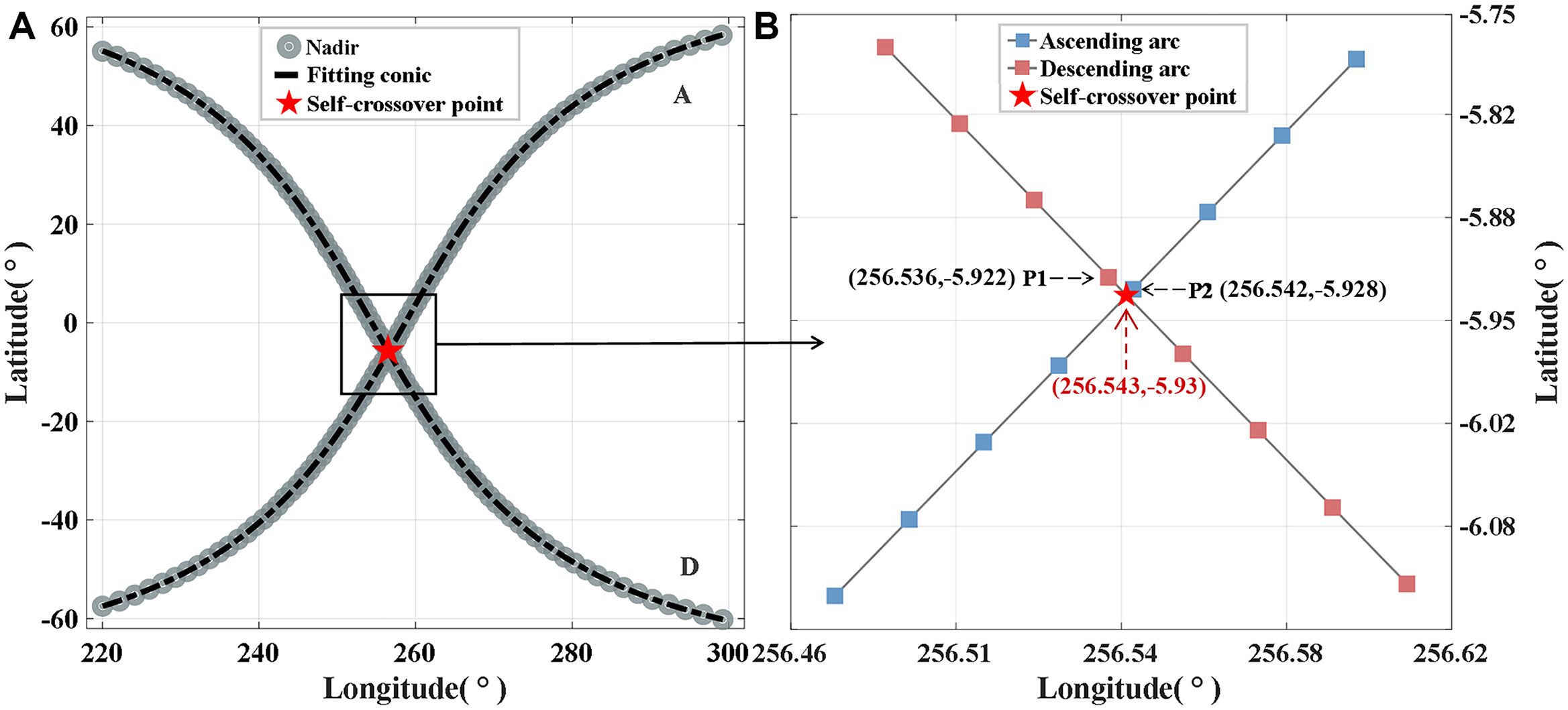
Figure 1. Extraction process of self-crossover points. (A) The intersecting ascending pass A and descending pass D are identified, and the presence of self-crossings is evident from the fitting curves. (B) P1 and P2 are the two closest nadir points on the two passes, using a total of 8 points before and after them to solve the orbit equation, and then calculate the self-crossover point.
At least eight consecutive nadir points are then recorded on both sides of P1, and the same for P2, which can ensure the accuracy and avoid the influence of near-shore areas. The orbit equations of the intersecting passes are constructed based on the nadir points. Subsequently, the latitude and longitude coordinates of the self-crossover points (as depicted in Figure 1B) can be determined by solving the transcendental equation.
Secondly, the Radial Basis Function (RBF) interpolation method is employed for interpolating the differences of SSH uncorrected for the SSB and the along-track data mentioned in Section 2.1 and 2.2 at the self-crossover points.
Finally, data quality control is also required to ensure the validity and reliability of the data, and the selection criteria are shown in Table 1 (Bosch and Savcenko, 2007; Ablain et al., 2010; Eum/Ops-Jas/Man, E. et al., 2021). Through the above filtering conditions, a total of 890,593 self-crossover points from global oceanic regions is selected as the original dataset of the neural network in this paper. The global distribution of self-crossover points is shown in Figure 2.
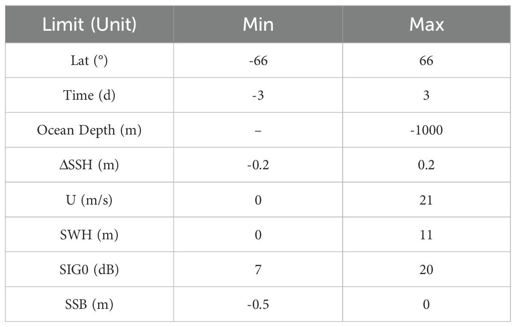
Table 1. Selection criteria.
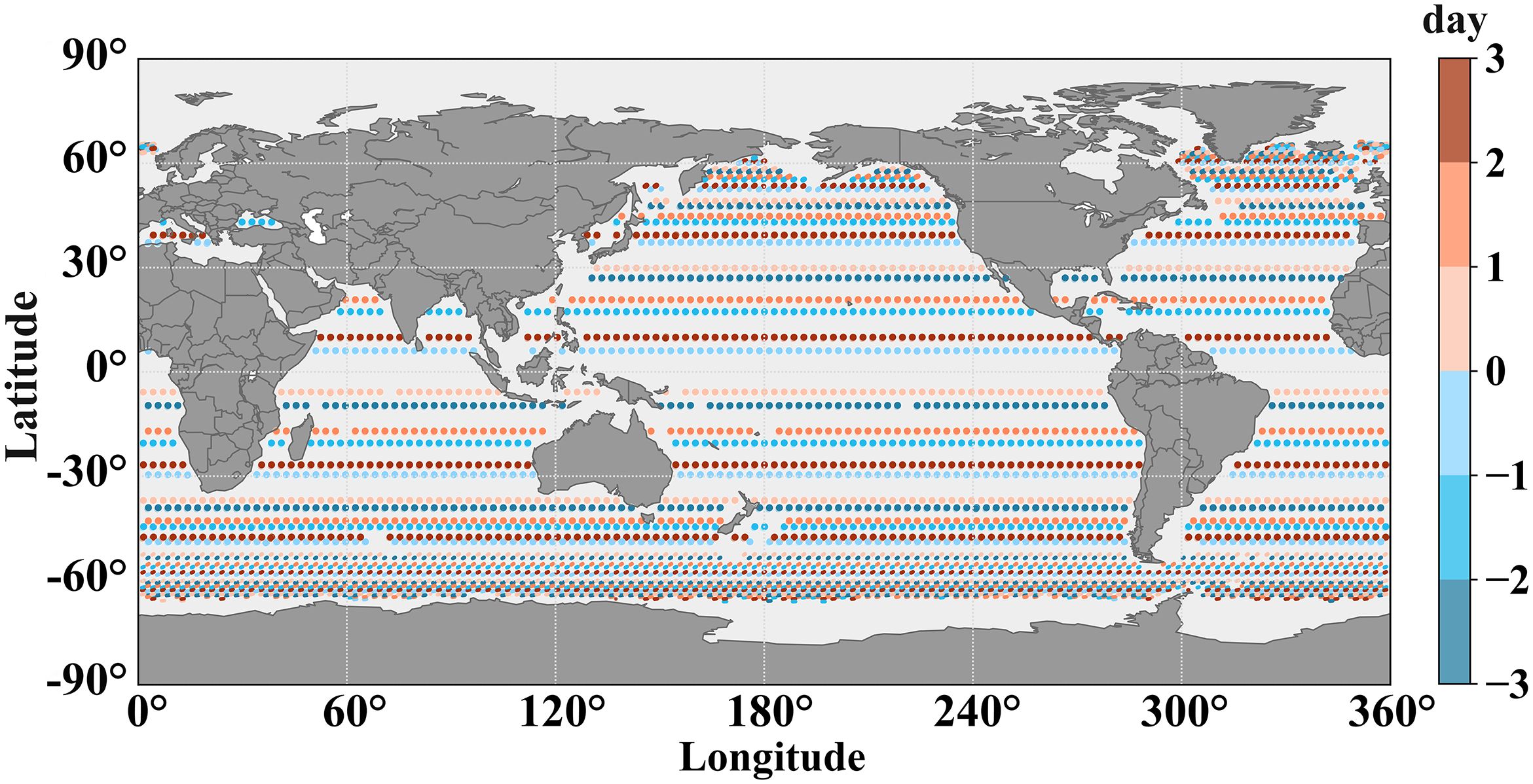
Figure 2. Global distribution of self-crossover points within three days. The time of ascending pass minus the time of descending pass is in the range of -3~3 days.
The differences of SSH measurement uncorrected for the SSB at the self-crossover points were always used for estimating the values of SSB in previous studies (Gaspar et al., 1994; Labroue et al., 2004). Similarly, their differences are also employed in this study. The SSH measurement at a given position can be represented as SSH’. SSH’ is calculated as shown in Equation 1:
where represents the geoid signal, η corresponds to the ocean dynamic topography, and ω denotes the measurement noise.
The association between the sea state-related variable and the can be mathematically represented in Equation 2:
where denotes the mapping function, and is a constant that ensures the equation holds.
The difference at the self-crossover points can be expressed as Equation 3:
where , , and the indices 1 and 2 are used to denote the ascending and descending passes at the self-crossover points, respectively.
The geoid signal () described by Equation 1 can be effectively eliminated by calculating the at the same location. The time difference between two measurements at the self-crossover points is strictly limited to 3 days, ensuring that any changes of the ocean dynamic topography () in Equation 1 is negligible within this specific time frame (Wang et al., 2021). The measurement error (ω) in Equation 1 consists mainly of errors in the dry and wet troposphere, ionosphere, ocean tide, pole tide, solid earth tide, and dynamic atmospheric pressure, and instrument noise in addition to the SSB. Except for the instrument noise, the other error terms can be corrected by the corresponding correction models. And under the tentative assumption of a weak dependence on sea state effects, the convergence terms of and in Equation 3 towards zero mean values (Vandemark et al., 2002; Tran et al., 2010). Sentinel-6 has the advantage of high performance and low instrument noise compared to Jason-3 and Sentinel-3. Its measurement noise can be suppressed down to 0.5 cm, approximately one-fiftieth that of SSB (Donlon et al., 2021). Therefore, in Equation 3, the ΔSSH can be regarded as the observation sample values of the ΔSSB.
From Section 3.1, it is evident that the key objective of the SSB estimation model is to establish the appropriate mapping function between the variables X and SSB. This requirement can be fulfilled by employing the Multilayer Perceptron (MLP) model. Siamese networks are able to generate a similarity function from pairs of input data, where subnetworks share the same weights to produce a single output. In our study, it is necessary to estimate SSB values in pairs based on paired data of self-crossover points and correct ΔSSB using the ΔSSH, which corresponds exactly to the Siamese network structure. And Siamese networks perform better as compared to other similarity learning techniques (Nandy et al., 2020), mainly due to their generalization capability over similar datasets (Hoffer and Ailon, 2015). Therefore, the Siamese network framework is adopted in our research. Within this framework, two MLP models are employed to develop the SSB estimation model, both of which have the identical structure as well as share weights and biases.
Figure 3 depicts the model training methodology. The dataset covering the period from 2021 to 2023 are pre-processed according to the methods in Section 2.3 and then shuffled. Subsequently, it is divided into separate training dataset and validation dataset. The train dataset is employed for model training, while the validation dataset is used for assessing the correctness of the SNSSB. The data for a full year in 2022 are all classified as test dataset after the same pre-processing and used to obtain the final output of the SNSSB.
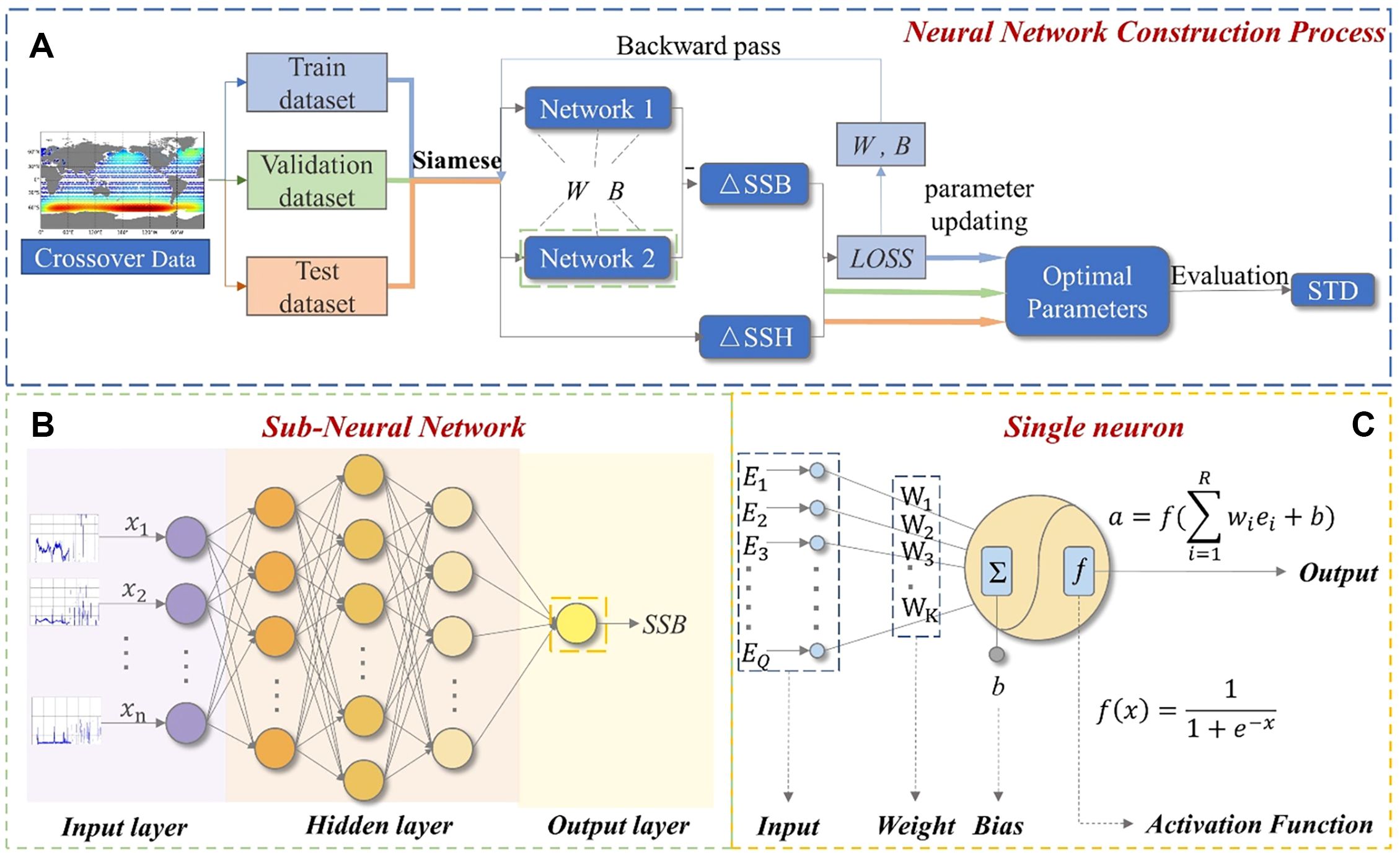
Figure 3. Scheme of sea state bias estimation model using Siamese network structural components. (A) Model construction process. (B) Structure of the sub-network. (C) Structure of the multi-input neuron. This neural network consists of one input layer, one output layer, and three hidden layers. Its activation function is Sigmoid and its loss function is MSE.
Combining Figures 3B, C, the input of neurons in the sub-neural network could be denoted by Equations 4, 5:
, where M is the number of layers of the neural network. serves as the input to the (m+1)th layer of the network, while and represent the outputs of the mth layer and (m+1)th layer of the network, respectively. The weight matrix of the (m+1)th layer of the network is denoted as , while the bias vector is denoted by . The activation function for the (m+1)th layer is expressed by . The initial input vector is , the chosen parameter vector, which provides the initial conditions for Equation 5. The output of the last layer of neurons is the final output of the subnetwork as .
The mean square error function is employed for the loss function in the training process, aiming to minimize it. The loss function, denoted as F, can be mathematically expressed as Equation 6:
where k represents the number of iterations, y is the corresponding target output.
Based on Equation 6, the weights and biases in the network are adjusted using the gradient descent rule, as shown in Equations 7, 8.
where represents the learning rate; represents the weight connecting the jth input of the mth layer and the ith neuron of the (m+1)th layer in the kth iteration of the network; represents the weight connecting the jth input of the mth layer and the ith neuron of the mth layer in the (k+1)th iteration of the network; denotes the bias of the ith neuron in the mth layer at the kth iteration of the network, while represents the bias at the (k+1)th iteration.
According to the chain rule, Equations 7, 8 can be simplified into matrix form as shown in Equations 9, 10:
Where Hm is calculated by Equation 11:
where Z indicates the number of neurons in the mth layer.
Applying the chain rule once again can give Equations 12–14:
where Z+1 indicates the number of neurons in the (m+1)th layer.
Combining Equations 12–14 yields Equations 15, 16:
This recursive relationship is represented in the final layer of the network as Equation 17:
Hence, the recurrence relation for the defined variable H can be expressed as Equation 18:
Based on the above derivation, the overall learning algorithm of the neural network is summarized as follows: First, the sea state-related data is initially fed into two MLP networks. Subsequently, forward propagation is performed on these networks to obtain the SSB difference at the self-crossover points; Second, the loss function measures the deviation between the value of the difference in SSH and the network output value obtained in the preceding step. This deviation is then propagated backward through the Siamese network into the MLP network; Finally, the biases and weights in the MLP networks are updated using the steepest descent rule, aiming to minimize the value of the loss function.
In this study, the SWH and U from altimeter data and MWP from ERA5 are extracted and divided into two different input combinations: 1) SWH and U; 2) SWH, U and MWP. In addition to the fundamental parameters, this study also introduces SWH_RMS and SIG0_RMS as additional predictive parameters, resulting in the third input combination: 3) SWH, U, MWP, SWH_RMS and SIG0_RMS. SWH_RMS and SIG0_RMS, as statistical metrics of 1 Hz data obtained from the corresponding 20 Hz data (Zhang et al., 2015), can be used to evaluate the discrete degree or amplitude magnitude of SWH and SIG0 data. Consistent with the research results of Queffeulou and others, at locations where SWH of Sentinel-6 fluctuates more, the corresponding SWH_RMS values are also larger, especially where anomalous peaks occur (Sepulveda et al., 2015; Queffeulou, 2016). Similar trends are observed between SIG0 and SIG0_RMS. Therefore, SWH_RMS and SIG0_RMS, as complementary information of wave state and scattering signals, can be considered as good indicators reflecting the quality of SWH and SIG0 measurements (Zhang et al., 2015). They can be used to mark these anomalous peaks to provide discriminative information for SIG0 and SWH to mitigate the effects of the associated anomalous peaks (Queffeulou, 2013). After data threshold screening, they can be further used to discriminate measurement anomalies caused by anomalous growth of the radar echo signals and strong rain attenuation, etc (Queffeulou, 2016). With SWH_RMS and SIG0_RMS as additional input variables, the network can utilize their information and backpropagation to adjust weights and biases of corresponding data features, helping to capture abnormal features of SWH and SIG0 data in order to better discriminate the true change patterns of the signals. This is expected to reduce interference and enhance robustness, thereby improving the accuracy and stability of the estimation. In Table 2, the names of the three different models obtained based on the input combinations are listed from top to bottom. Each model corresponds to a specific combination of input variables, as mentioned earlier.
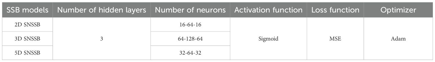
Table 2. Model parameters and optimal hyperparameters.
The SNSSB has two types of parameters: 1) optimal parameters derived during training; 2) hyperparameters that need to be defined before training (Alerskans et al., 2022). Various hyperparameters have a significant impact on the performance and efficiency of the model. In order to achieve the best balance between these two factors, extensive experimentation is conducted with different combinations of hyperparameters. These combinations are thoroughly evaluated using the training dataset, and the final hyperparameter configurations, deemed to strike a balance between performance and efficiency, are summarized in Table 2.
In SSB studies, SSH variance analysis is a customary practice due to the absence of underlying facts that can be used for validation. This study employs three evaluation parameters to assess the accuracy of SNSSB: the variance of the SSH difference at the self-crossover points, the explained variance, and the SSH variance difference index (SVDI).
First, following Tran’s method (Tran et al., 2010), variance serves as a fundamental metric for analysing the consistency of SSH between ascending and descending passes. The equation for calculating the variance is Equation 19:
where, M represents the overall amount of data, refers to the SSH corrected for SSB, and is the average of the values. As shown in Equation 19, smaller values of the variance indicate a higher accuracy of the SSB estimation model utilized.
Second, the explained variance serves as the primary metric for assessing the accuracy of the employed SSB estimation model (Gaspar and Florens, 1998; Tran et al., 2010). The concept of explained variance refers to the reduction in the variance of SSH differences resulting from the application of the provided SSB correction. The equation for the explained variance is Equation 20:
where denotes the difference in SSH uncorrected for SSB, denotes the difference in SSH corrected for SSB. The higher value of the explained variance indicates the greater accuracy of the SSB estimation model, as shown in Equation 20.
Third, like what Pires did (Pires et al., 2019), this paper utilize the SSH variance difference index (SVDI) as a metric to evaluate the performance of SSB estimation models. This index is estimated by calculating the scalar difference of SSH variance. The equation for calculating the SVDI is Equation 21:
where the reference dataset represents the SSH dataset, which are obtained from the SSB calculated using the NPSSB model. On the other hand, the dataset represents the SSH dataset obtained from the SSB calculated using the SNSSB. Based on Equation 21, it can be inferred that the higher SVDI value compared to the NPSSB model indicates that the SNSSB is more efficacious in minimizing the difference in SSH at the self-crossover points. In other words, the accuracy of SNSSB exceeds that of the traditional NPSSB model.
In this section, the lookup table for SSB is generated using SNSSB_2D with a resolution of 0.25 m/s × 0.25m. The 2D SNSSB is constructed based on the ΔSSH. The SSB are visually represented in Figure 4 as a 2D grid, with contours indicating the values in centimetres (cm).
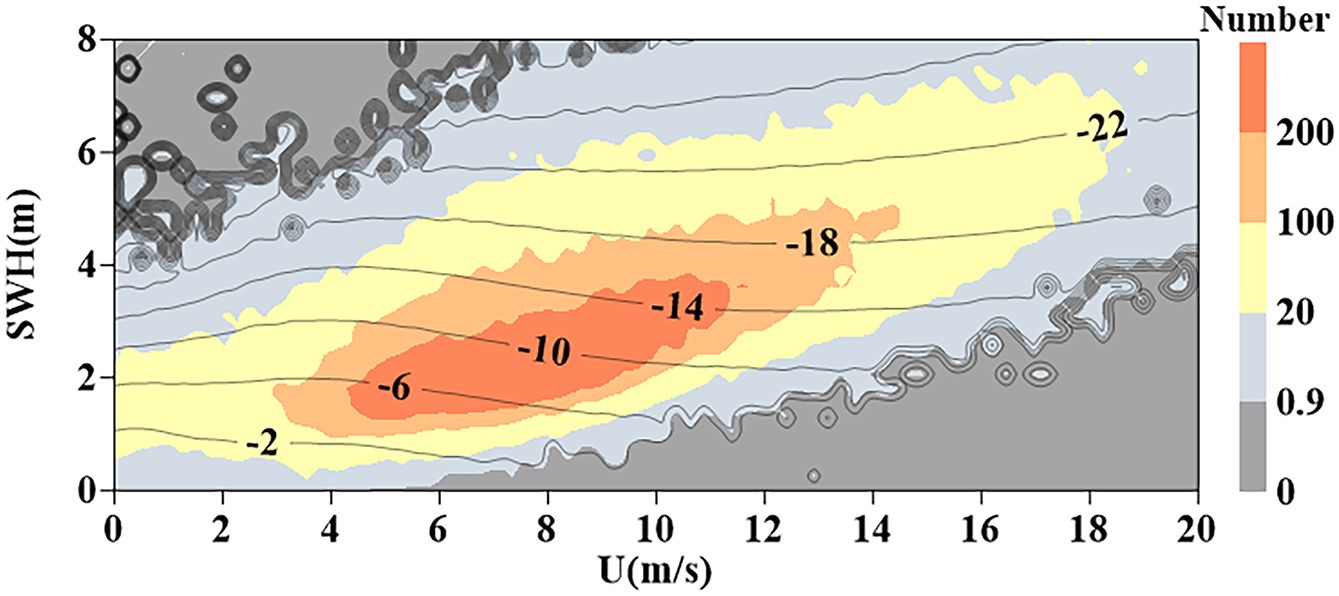
Figure 4. SSB estimates (in cm) obtained by 2D SNSSB. Basemap color represents data density. Dark gray, light gray, yellow, radish yellow, and orange represent areas with no data, areas with less than 20 data, areas with less than 100 data, areas with less than 200 data, and areas with more than 200 data per bin, respectively. The color grading method is employed as a guiding framework for subsequent color grading.
As evident from Figure 4, the value of SSB shows a clear decreasing trend with the increase of SWH, while its association with the second parameter U of interest is relatively weak. Furthermore, upon examining Figure 4, when the SWH is given, the value of SSB initially tends to increase in the region of low U. As the U increases, the value of SSB then starts to decrease.
The 3D SNSSB generates a 3D lookup table. To ensure an adequate number of measurement points in the respective plane, three fixed values are selected near the average values of SWH, U, and MWP. To better represent the 3D lookup table, this study presents the SSB as 2D array by holding the third parameter. The obtained results are presented in Figure 5. Figure 5A exhibit a high level of agreement with Figure 4. Figure 5B show that the relationship between the magnitude of SSB and MWP is also relatively weak, and distinct differences in the impacts of U and MWP on SSB can be observed when compared with Figure 5A. The value of the SSB increases with an increase in the MWP. Figure 5C illustrates the distribution of SSB estimates within the (U, MWP) plane. In the data-rich area, when the SWH is held constant, the variation of SSB with the MWP is more prominent compared to the variation with the U.
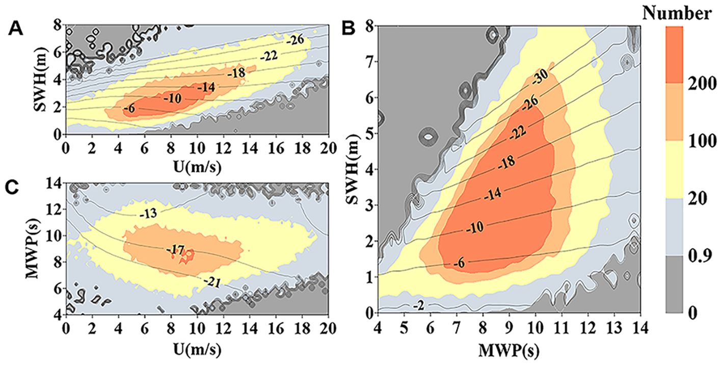
Figure 5. SSB estimates (in cm) obtained by 3D SNSSB. The fixed values are (A) MWP = 9s, (B) U=9m/s, (C) SWH = 4m, respectively.
The 5D SNSSB generates a 5D lookup table based on the variables of SWH, U, MWP, SWH_RMS, SIG0_RMS. Fixed values are selected around the average value of each of the five parameters to ensure that sufficient data are available. To illustrate the 5D lookup table, this study presents the SSB in 2D form by fixing the values of the three additional parameters. Figures 6A–C are selected to depict the same parameters as Figure 5, and it demonstrates excellent agreement with Figure 5. The distribution patterns observed in both figures remain consistent.
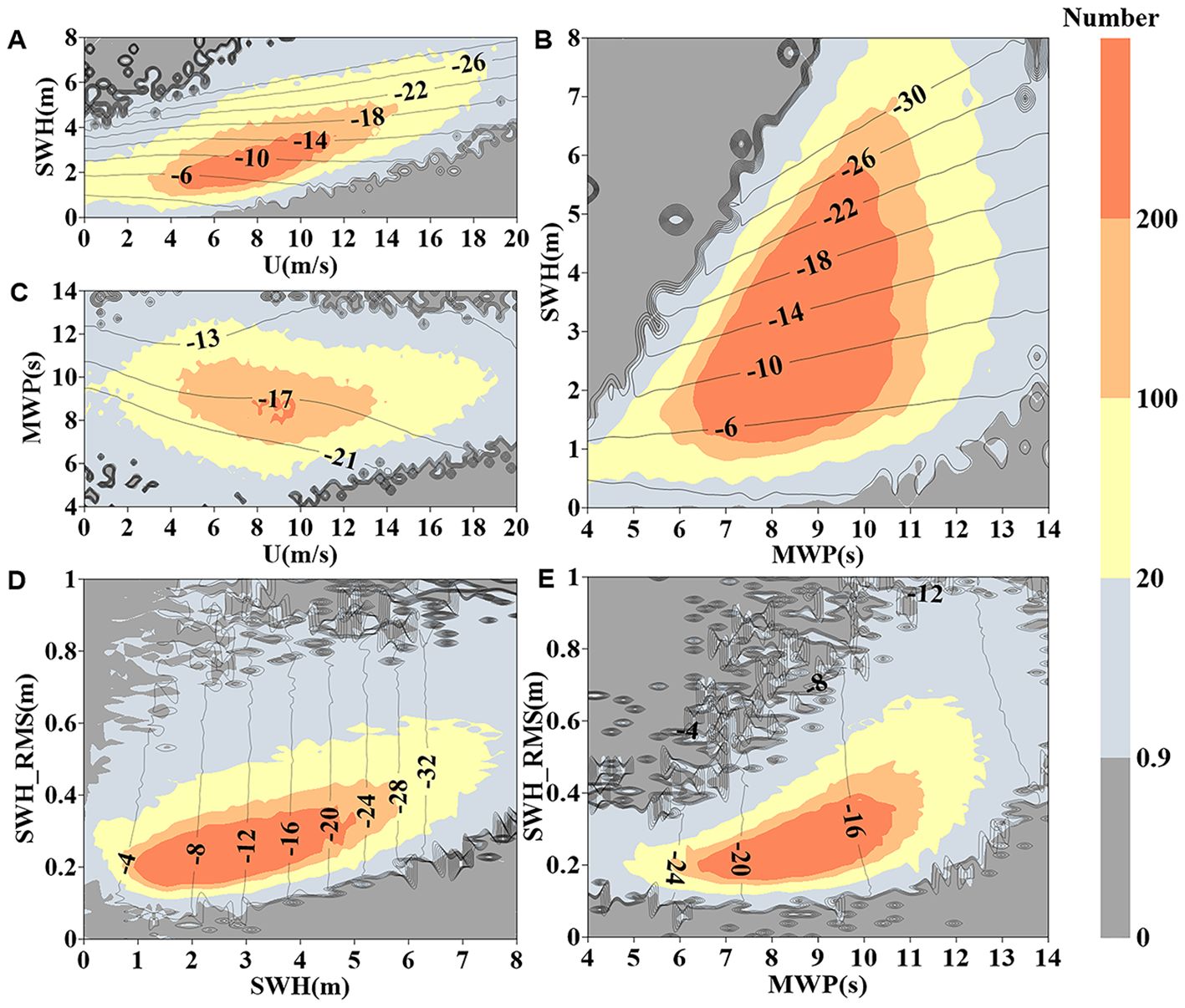
Figure 6. SSB estimates (in cm) obtained by 5D SNSSB. The remaining three variables are fixed at constant values in each subgraph from (A–E) to present the SSB estimates in two dimensions. The fixed values are U= 9 m/s, SWH = 4 m, MWP = 9 s, SWH_RMS = 0.31 m, and SIG0_RMS = 0.08dB, respectively.
Figure 6D represents the combination of SWH_RMS and SWH, while Figure 6E represents the combination of SWH_RMS and MWP. Figures 6D, E offer compelling visual evidence supporting the notion that SSB can be regarded as a decreasing function of SWH, while it exhibits a increasing trend with increasing MWP. Meanwhile, based on Figure 6, it can be observed that the individual impact of the newly added predictors on SSB is relatively small. Nevertheless, incorporating these predictors into the model contributes to obtaining more accurate SSB estimates. Therefore, their inclusion is significant in improving the overall accuracy of SSB estimation.
The SNSSB and NPSSB are tested for comparison using the dataset in Section 3.2. In evaluating the performance of 2D SNSSB, the SSB is calculated with the 2D NPSSB serving as a reference value for comparison, thereby comparing the utility of two SSB estimation methods. Likewise, when assessing the performance of 3D SNSSB, the SSB is calculated using the 2D SNSSB as a reference. And the SSB is calculated using the 3D SNSSB as a reference value for evaluating the performance of the 5D SNSSB, allowing for a comparison of the effects of different combinations of dimensional parameters on the SSB estimation.
Figure 7 displays the distributions of SSB values estimated by SNSSB and NPSSB. It reveals a close alignment of most data pairs with the ““ line, signifying a high degree of correlation among the SSB values obtained from different models. However, there are still a few data points that show asymmetry in the distribution on both sides of the ““ line.
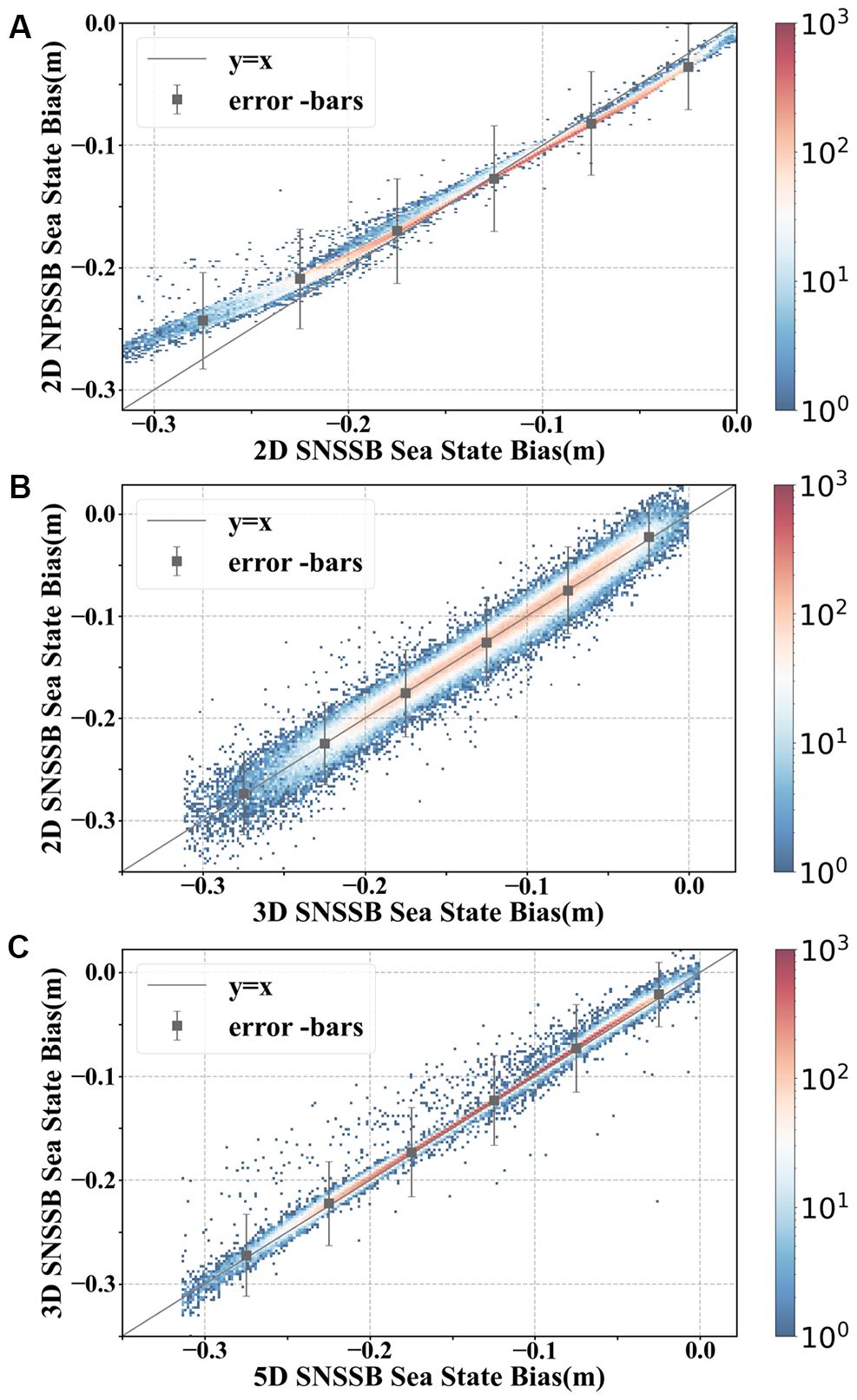
Figure 7. Comparison of SNSSB calculation results and NPSSB model calculation results under different input combinations. (A) SWH and U. (B) SWH, U and MWP. (C) SWH, U, MWP, SWH_RMS and SIG0_RMS. The black line represents the reference line “ “. The error -bars (mean ± 3*standard deviation) are overlaid at every 0.05 m of SSB.
This pattern can be explained by the relatively rare presence of areas with high SSB (< -0.25m) and low SSB (-0.05~0 m) in the ocean region.
Table 3 shows the comprehensive performance of SNSSB, compared to the NPSSB model. The overall bias of the SNSSB from the NPSSB model are observed to be -0.041 cm, -0.037cm and 0.020cm, respectively. Additionally, the standard deviations of the SNSSB from the NPSSB model are found to be 1.325 cm, 1.675 cm, and 1.756 cm, respectively. Based on the obtained values, it can be concluded that the SNSSB and NPSSB model exhibit a strong correlation and demonstrate similar results.

Table 3. Statistics of SNSSB/NPSSB models’ differences.
In this section, the accuracy of different models is compared by the variance and explained variance of the SSH difference at the self-crossover points, which are introduced in Section 3.4, as the evaluation criteria. The explained variance is computed using the global dataset for the year 2022. The data is divided into 10° latitude bands within the range of 66°S to 66°N to calculate individually the explained variance for each band. In Figure 8, the latitudinal distribution of the explained variance is depicted using four models.
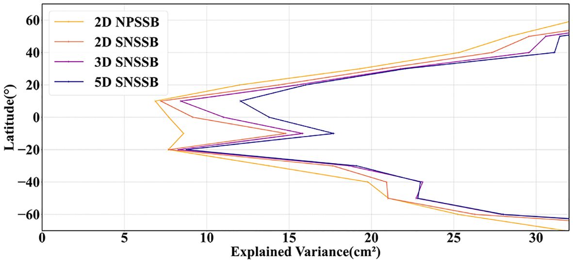
Figure 8. Meridional distribution of the variance explained by the 2D NPSSB, 2D SNSSB, 3D SNSSB and 5D SNSSB, respectively. Results are derived by partitioning the crossover differences data for 2022 into 10° latitude bands. Subsequent explained variance results are divided in this manner.
As shown in Table 4, compared with the 2D NPSSB, the variance of the ΔSSH of 2D SNSSB reduces 3.08 cm2, a 11.87% decrease. Therefore, the 2D SNSSB demonstrates higher accuracy compared to the 2D NPSSB and exhibits the significant improvement in accuracy. Figure 8 clearly shows that 2D SNSSB outperforms 2D NPSSB in terms of explained variance at different latitudes, indicating its effectiveness in capturing the underlying patterns of SSB. In particular, the SNSSB model demonstrates superior performance, especially in mid-latitude regions.
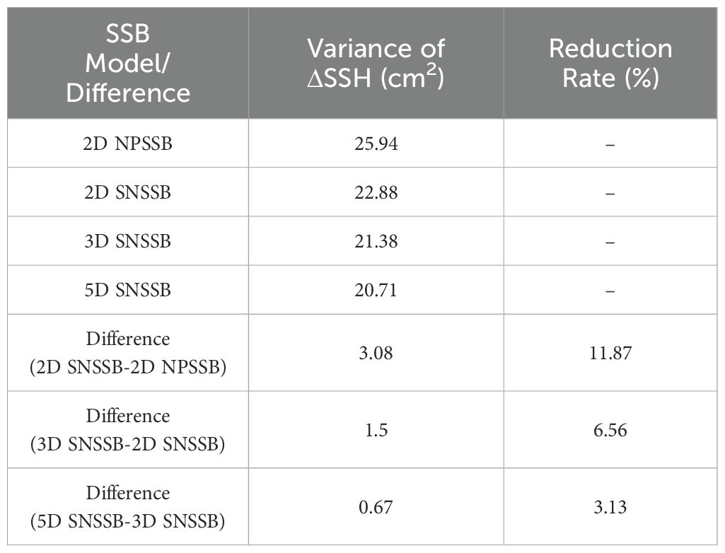
Table 4. Model variance and inter-model variance reduction.
The addition of the third parameter related to waves, such as MWP, has shown improved performance for 3D SNSSB estimation compared to 2D SSB estimation. According to the information provided in Table 4, compared to the 2D SNSSB, the variance of ΔSSH of 3D SNSSB reduces 1.5 cm2, a 6.56% decrease. Then compared to the 2D NPSSB, the variance is reduced by 17.66%. Observing Figure 8, it becomes apparent that the 3D SNSSB has a higher explained variance than the 2D models in all latitude bands. Indeed, in the region between 30°S and 30°N, the difference in explained variance between the 2D and 3D SNSSB is relatively small, and the trends are similar. This suggests that both models have similar performance in models. Using the 5D SNSSB, the variance of the ΔSSH is reduced by 0.67cm2 compared to the 3D SNSSB, a decrease of 3.13%. Compared to the 2D NPSSB, the variance is reduced by 20.24%. According to Figure 8, the explained variance clearly shows that the 5D SNSSB achieves higher values, especially in the region between 10°S and 10°N. The above demonstrates that the inclusion of two additional parameters in the 5D SNSSB enhances its accuracy and validity in estimating the SSB.
In addition, a comparative validation experiment is presented to help assess the accuracy of the SNSSB models. The SSH values from Surface Water and Ocean Topography (SWOT), renowned for higher measurement accuracy, are taken as the reference value in the verification experiment. The crossover point dataset is constructed using the Sentinel-6 and SWOT data in March 2024 in a similar way as in Section 2.3, without distinguishing between ascending and descending passes, resulting in a total of 116,680 crossover points. Taking the corrected SSH values of SWOT at the crossover points as the evaluation benchmark, the corrected SSH values of Sentinel-6 applying different SSB models are evaluated. The variance of the ΔSSH at the crossover points serves as an evaluation metric for the auxiliary validation of the models. The smaller the variance, the better the correction result of the model.
The validation results are as follows: the variances between the SSH of Sentinel-6, corrected by applying different SSB models (2D NPSSB, 2D SNSSB, 3D SNSSB, and 5D SNSSB), and the SSH of SWOT are 21.71 cm2, 20.01 cm2, 19.09 cm2, and 18.48 cm2, respectively. Compared to the 2D NPSSB model, the 2D SNSSB, 3D SNSSB, and 5D SNSSB models reduce the variance by 7.83%, 12.07%, and 14.89%, respectively. The variances of SNSSB models all decrease compared to the 2D NPSSB model, and the variances of the corresponding models decrease progressively with higher dimensions of variables, indicating improved performance in these models. Among them, the 5D SNSSB model exhibits the best performance. These results confirm the effectiveness of the SNSSB models and the advantages of the 5D SNSBB model.
The global distribution of SVDI among different models is analysed in 10° latitude bands, with quantification and meticulous calculation of data within each band, followed by obtaining SVDI values for each latitude band. These calculated values are then visualized using a histogram. Positive SVDI values indicate improvements in the accuracy of the model estimation compared to the reference model, and the larger the magnitude, the better the improvement. Conversely, negative SVDI values indicate the opposite.
Figure 9 shows the spatial evaluation of SSH differences at self-crossover points using SVDI in the latitudinal direction. All models are calculated using the 2D NPSSB model as a reference, and the results of the calculations are positive. Overall, it is evident that all SNSSB models outperform the 2D NPSSB model in the latitudinal direction, especially near the equator and in the high latitude regions of the southern hemisphere, where higher SVDI values (around 30%) are calculated. This indicates that compared to NPSSB model, the SNSSB models boost significantly in these latitude intervals, which is consistent with the findings in Figure 8.
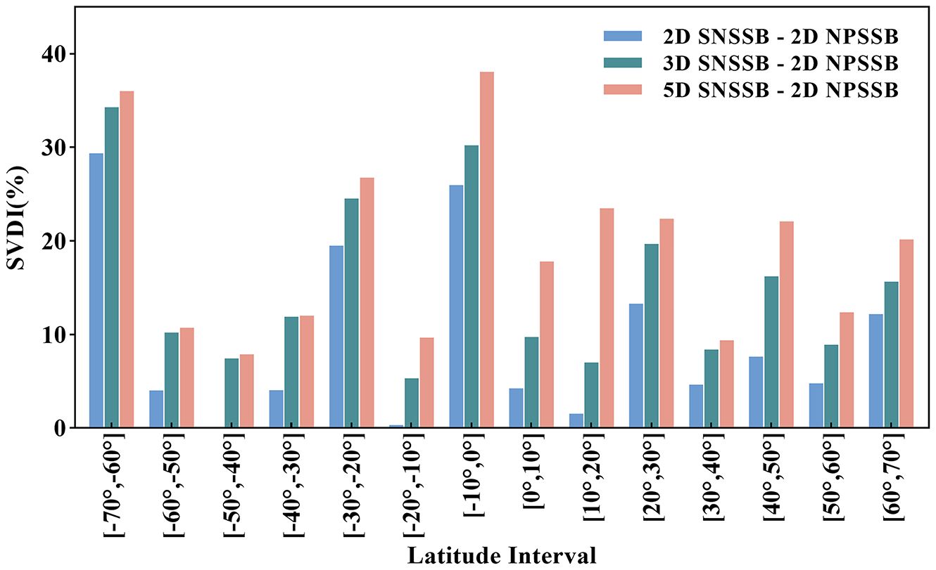
Figure 9. Variation of SVDI values with latitude obtained using each SNSSB model (2D, 3D, and 5D) in comparison to the 2D NPSSB benchmark. A positive SVDI value indicates that the model outperforms the benchmark, while a negative SVDI indicates the opposite.
Compared to the 2D SNSSB model, the 3D SNSSB model shows improvements across all latitude intervals and performs well overall, demonstrating an average improvement of approximately 5%, with enhancements of up to 10% observed in the mid-latitudes of the northern hemisphere. This suggests that the inclusion of wave-related parameters, such as MWP, can improve the accuracy of SSB estimation, which is consistent with findings from previous studies. Compared to the 3D SNSSB model, the 5D SNSSB model also exhibits improvements across all latitude intervals, but the northern hemisphere outperforms the southern hemisphere, and some latitude intervals can even be improved by about 15%. This further illustrates the superiority of the five-dimensional model. It follows that as the relevant variables increase, the models of the corresponding dimensions also show better advantages.
Theoretically, the five-dimensional model optimizes and complements the information from the three-dimensional model by incorporating variables describing the fluctuation states of SWH and SIG0. In practical applications, these five parameters can be directly obtained from satellite data. On the other hand, the five-dimensional model outperforms the three-dimensional model in terms of both the results of the three types of evaluation indices and the validation results using SWOT as a reference. It can be concluded that the five-dimensional model is more capable of improving the accuracy of synthetic aperture radar altimetry in practical applications.
Since SSB models are estimated over the global open ocean, the global SSB model may not adequately represent the regional characteristics of specific wind and wave conditions. Passaro et al (Passaro et al., 2016, 2018). constructed and analysed regional SSB models using both parametric and non-parametric approaches. Based on this rationale, the Kuroshio Extension (KE, 20-45°N, 125-155°E) and Gulf Stream Extension (GSE, 20-45°N, 60-90°W) were selected for their distinct wind, wave, and current conditions, as well as relatively abundant in-situ measurements, to construct SSB models for exploring their SSB characteristics. Taking the combination of U and SWH parameters as an example, the constructed SNSSB model and NPSSB model are compared and analysed using the regional data from 2022.
In Table 5, the variance of ΔSSH is reported after applying different SSB corrections models for two regions. The regional models decrease the variance of ΔSSH by over 10%, representing a significant correction for regional sea state, and the SNSSB model is more effective in reducing variance than the NPSSB model. In addition, the performance of both models in the Gulf Stream Extension is better than that in the Kuroshio Extension, indicating the sea state in the latter may exhibit greater variability and greater complexity, and illustrating the value of regional sea state bias studies.
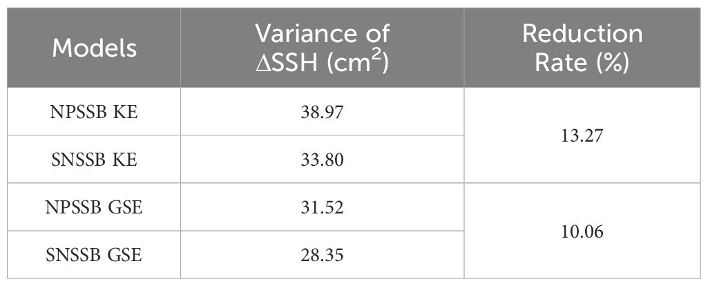
Table 5. Regional model variance.
Figure 10 presents the application results of the NPSSB model from two regions and the SNSSB model from the same regions. Figure 10A shows that the SNSSB model can achieve better results than the operational products with a smaller amount of data, converging within 8 cycles, while the NPSSB model requires more cycles to converge and ultimately has weaker convergence than the SNSSB model. Moreover, the Gulf Stream Extension outperforms the Kuroshio Extension in both models, which also corroborates the data in Table 5, showing different SSB characteristics between the two regions.
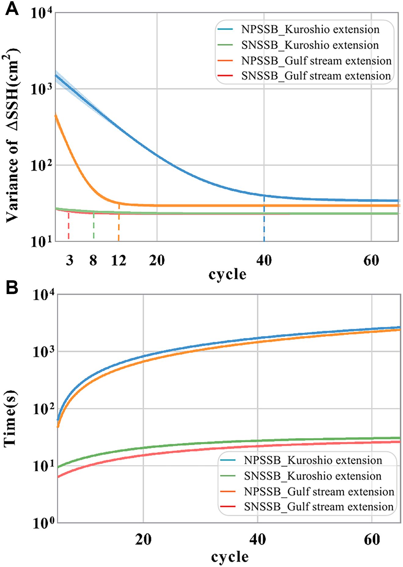
Figure 10. Demonstration of the application results of regional SNSSB models and NPSSB models: (A) Plot of the convergence curves for the Variance of ΔSSH. The vertical straight lines, corresponding to the colors of the convergence curves, mark the positions of the inflection points for the four regional SSB models. (B) Plot of efficiency computation.
Figure 10B illustrates that the newly proposed SNSSB model, in addition to the significant improvement in results, demonstrates a substantial increase in computational efficiency compared to the NPSSB model with the Nadaraya-Watson (NW) estimator. This efficiency improvement is another major benefit of the SNSSB model. The used computer configuration comprises an Intel(R) Xeon(R) Central Processing Unit (CPU) E5-2673 v4 @ 2.30 GHz and the 128 GB of Random-Access Memory (RAM). Compared to NPSSB, the computational efficiency of SNSSB has been enhanced by over 100 times. Moreover, even with an increase in input vector dimensionality, the computation time of global SNSSB remains within tens of minutes, indicating minimal impact.
As mentioned in the introduction, estimation of SSB typically depends on empirical models due to the incomplete state of the physical theory of SSB and the unclear mechanisms related to sea state variables (Tran et al., 2010). However, operational NPSSB models, constrained by its solution method, exhibits limitations in exploring the multiple influences on SSB. Therefore, we propose a deep learning approach (SNSSB) as a solution. Based on the data characteristics at the self-crossover points and the SSB estimation formula, this paper employs a combination of Siamese network architecture and MLP to construct the SSB estimation models. The models take multi-dimensional relevant sea state variables as input, the difference between Siamese SSB values that share the structure and parameters as output, and the SSH difference as label, which can further improve the accuracy of SSB.
Results indicate that, in the global region, compared to traditional 2D NPSSB, 2D SNSSB not only decreases the variance of the SSH difference by 11.87%, but also improves the explained variance, especially by approximately 5 cm2 in mid- and low-latitude regions. This shows that SNSSB has more advantages compared with NPSSB. 3D SNSSB shows advantages over 2D SNSSB in all three metrics, which is aligning with previous research results in NPSSB, illustrating the complexity and uncertainty of SSB composition. Therefore, the introduction of more relevant variables is helpful to explore the influencing factors of SSB. 5D SNSSB also exhibits advantages over 3D SNSSB in all three metrics, indicating that incorporating SWH_RMS and SIG0_RMS can enhance the reliability and accuracy of Synthetic Aperture Radar altimeter SSB. This enhancement may be attributed to the fact that they provide complementary information on wave and wind speeds. Moreover, 5D SNSSB performs best in validation using the SSH values of SWOT as a reference. SNSSB has also shown considerable potential and advantages for SSB research within small sample areas. Due to the different wind and wave conditions in the region, SNSSB can use fewer data to obtain more accurate and effective regional SSB estimates. In the regions of Gulf Stream Extension and Kuroshio Extension selected in this study, SNSSB can both reduce the variance of the SSH difference by more than 10% compared to NPSSB. We also found that the correction results for the Gulf Stream Extension are better than those for the Kuroshio Extension. This may be because the Kuroshio Extension has more complex sea state and is more influenced by wind than the Gulf Stream Extension. This suggests that the performance of SSB varies from region to region, so further studies on regional SSB are necessary. Additionally, SNSSB can improve the computational efficiency by approximately 100 times compared with NPSSB.
This article does not offer more in-depth scientific explanations about the physical mechanisms between the relevant sea state variables and the SSB, as well as the physical causes of the regional variations, which may confuse many physical oceanographers who want to seek the relevant physical mechanisms. This is also the difficulty in current SSB research. Therefore, improving the interpretability of deep learning, deepening our understanding of the oceanographic mechanisms, and continuing to dig into the physical causes of regional changes are directions for continued research.
But it is undeniable that this study provides a fast and feasible method to explore multi-dimensional physical factors associated with SSB. As an innovative attempt, SNSSB is not the ultimate solution. There are still numerous areas for improvement. As Sentinel-6 releases more data, we will continue to enrich the dataset and update the model results. Further research could focus on applying the model to other satellite data, testing relevant variables, and assessing the quality of variable data sources.
The original contributions presented in the study are included in the article/supplementary material. Further inquiries can be directed to the corresponding author.
CM: Funding acquisition, Methodology, Supervision, Writing – original draft, Writing – review & editing. QH: Data curation, Investigation, Software, Writing – original draft. CL: Data curation, Investigation, Software, Writing – original draft. YL: Supervision, Validation, Writing – review & editing. YD: Supervision, Validation, Writing – review & editing. CZ: Supervision, Validation, Writing – review & editing. GC: Supervision, Validation, Writing – review & editing.
The author(s) declare financial support was received for the research, authorship, and/or publication of this article. This work was financially supported by the National Natural Science Foundation of China (42276179), Laoshan Laboratory Science and Technology Innovation Projects (LSKJ202201302), Laoshan Laboratory Science and Technology Innovation Projects (LSKJ202204301) National Natural Science Foundation of China (42030406), and in part by the Taishan Scholars Program.
The authors declare that the research was conducted in the absence of any commercial or financial relationships that could be construed as a potential conflict of interest.
All claims expressed in this article are solely those of the authors and do not necessarily represent those of their affiliated organizations, or those of the publisher, the editors and the reviewers. Any product that may be evaluated in this article, or claim that may be made by its manufacturer, is not guaranteed or endorsed by the publisher.
Ablain M., Philipps S., Picot N., Bronner E. (2010). Jason-2 global statistical assessment and cross-calibration with Jason-1. Mar. Geod. 33, 162–185. doi: 10.1080/01490419.2010.487805
Alerskans E., Zinck A.-S. P., Nielsen-Englyst P., Høyer J. L. (2022). Exploring machine learning techniques to retrieve sea surface temperatures from passive microwave measurements. Remote Sens. Environ. 281, 13. doi: 10.1016/j.rse.2022.113220
Andersen O. B., Scharroo R. (2011). “Range and geophysical corrections in coastal regions: And implications for mean sea surface determination,” in Coastal Altimetry. Eds. Vignudelli S., Kostianoy A. G., Cipollini P., Benveniste J. (Springer, Berlin Heidelberg), 103–145. doi: 10.1007/978-3-642-12796-0_5
Badulin S. I., Grigorieva V. G., Shabanov P. A., Sharmar V. D., Karpov I. O. (2021). Sea state bias in altimetry measurements within the theory of similarity for wind-driven seas. Adv. Space Res. 68, 978–988. doi: 10.1016/j.asr.2019.11.040
Bosch W., Savcenko R. (2007). “Satellite altimetry: Multi-mission cross calibration,” in IAG Symposium on Dynamic Planet, vol. 130 . Eds. Tregoning P., Rizos C. (Springer-Verlag Berlin, Cairns, Australia. Berlin), 51–56. doi: 10.1007/978-3-540-49350-1_8
Chelton D. B. (1994). The sea state bias in altimeter estimates of sea level from collinear analysis of TOPEX data. J. Geophys. Res. Oceans. 99, 24995–25008. doi: 10.1029/94JC02113
Coleman R. (2001). Satellite altimetry and earth sciences: A handbook of techniques and applications. EOS Trans. Am. Geophys. Union. 82, 376–376. doi: 10.1029/01EO00233
Donlon C. J., Cullen R., Giulicchi L., Vuilleumier P., Francis C. R., Kuschnerus M., et al. (2021). The Copernicus Sentinel-6 mission: Enhanced continuity of satellite sea level measurements from space. Remote Sens. Environ. 258, 112395. doi: 10.1016/j.rse.2021.112395
Dumont J. P., Rosmorduc V., Picot N., Desai S., Boneamp H., et al. (2017). Sentinel-3 SRAL Marine User Handbook. Version 1.0-A. Available online at: https://earth.esa.int/eogateway/documents/20142/1564943/Sentinel-3-SRAL-Marine-User-Handbook.pdf. (Accessed [Sep. 15, 2023]).
Dumont J. P., Rosmorduc V., Picot N., Desai S., Boneamp H., et al. (2018). Sentinel-6 End User Requirements Document EURD. Version 3.0-E. Available online at: https://earth.esa.int/eogateway/documents/20142/1557871/Sentinel-6-End-User-Requirements-Document-EURD.pdf. (Accessed [Sep. 17, 2023]).
Eum/Ops-Jas/Man, E, Dumont J. P., Rosmorduc V., Picot N., Desai S., Boneamp H., et al. (2021). Jason-3 Products Handbook. Version 2.0-1. Available online at: https://www.ospo.noaa.gov/Products/documents/hdbk_j3.pdf. (Accessed [Apr. 17, 2023]).
Gaspar P., Florens J. (1998). Estimation of the sea state bias in radar altimeter measurements of sea level: Results from a new nonparametric method. J. Geophys. Res. Oceans. 103, 15803–15814. doi: 10.1029/98JC01194
Gaspar P., Labroue S., Ogor F., Lafitte G., Marchal L., Rafanel M. (2002). Improving nonparametric estimates of the sea state bias in radar altimeter measurements of sea level. J. Atmos. Oceanic Technol. 19, 1690–1707. doi: 10.1175/1520-0426(2002)019<1690:INEOTS>2.0.CO;2
Gaspar P., Ogor F., Le Traon P., Zanife O. (1994). Estimating the sea state bias of the TOPEX and POSEIDON altimeters from crossover differences. J. Geophys. Res. Oceans. 99, 24981–24994. doi: 10.1029/94JC01430
Ghavidel A., Schiavulli D., Camps A. (2016). Numerical computation of the electromagnetic bias in GNSS-R altimetry. IEEE Trans. Geosci. Remote Sens. 54, 489–498. doi: 10.1109/TGRS.2015.2460212
Glazman R. E., Greysukh A., Zlotnicki V. (1994). Evaluating models of sea state bias in satellite altimetry. J. Geophys. Res. 99, 12581–12591. doi: 10.1029/94JC00478
Glazman R. E., Srokosz M. A. (1991). Equilibrium wave spectrum and sea state bias in satellite altimetry. J. Phys. Oceanogr. 21, 1609–1621. doi: 10.1175/1520-0485(1991)021<1609:EWSASS>2.0.CO;2
Greene C. A., Gwyther D. E., Blankenship D. D. (2017). Antarctic mapping tools for MATLAB. Comput. Geosci. 104, 151–157. doi: 10.1016/j.cageo.2016.08.003
Haykin S. (2007). Neural Networks: A Comprehensive Foundation. 3rd Edition (USA: Prentice-Hall, Inc).
Hoffer E., Ailon N. (2015). “Deep metric learning using triplet network,” in Similarity-Based Pattern Recognition. Eds. Feragen A., Pelillo M., Loog M. (Springer International Publishing, Cham), 84–92. doi: 10.1007/978-3-319-24261-3_7
Jiang M., Xu K., Liu Y., Wang L. (2016). Estimating the sea state bias of Jason-2 altimeter from crossover differences by using a three-dimensional nonparametric model. IEEE J. Sel. Top. Appl. Earth Obs. Remote Sens. 9, 5023–5043. doi: 10.1109/JSTARS.2016.2557839
Kuo Y.-M., Liu C.-W., Lin K.-H. (2004). Evaluation of the ability of an artificial neural network model to assess the variation of groundwater quality in an area of blackfoot disease in Taiwan. Water Res. 38, 148–158. doi: 10.1016/j.watres.2003.09.026
Labroue S., Gaspar P., Dorandeu J., ZANIFé O., Mertz F., Vincent P., et al. (2004). Nonparametric estimates of the sea state bias for the Jason-1 radar altimeter. Mar. Geod. 27, 453–481. doi: 10.1080/01490410490902089
Li X., Zhang S., Geng T., Li J., Zhu B., Liu L., et al. (2022). An improved algorithm for extracting crossovers of satellite ground tracks. Comput. Geosci. 166, 9. doi: 10.1016/j.cageo.2022.105179
Masson-Delmotte V., Zhai P., Pirani A., Goldfarb L., Chen Y., Yu R., et al. (2021). “Summary for policymakers,” in Climate Change 2021 – The physical science basis: Working group I contribution to the sixth assessment report of the intergovernmental panel on climate change (Cambridge University Press, Cambridge), 3–32. doi: 10.1017/9781009157896.001
Melville W. K., Felizardo F. C., Matusov P. (2004). Wave slope and wave age effects in measurements of electromagnetic. J. Geophys. Res. Oceans. 109, 15. doi: 10.1029/2002JC001708
Miao H., Guo Y., Zhong G., Liu B., Wang G. (2018a). A novel model of estimating sea state bias based on multi-layer neural network and multi-source altimeter data. Eur. J. Remote Sens. 51, 616–626. doi: 10.1080/22797254.2018.1465361
Miao X., Miao H., Jia Y., Guo Y. (2018b). Using a stacked-autoencoder neural network model to estimate sea state bias for a radar altimeter. PloS One 13, 10. doi: 10.1371/journal.pone.0208989
Millet F. W., Arnold D. V., Warnick K. F., Smith J. (2003). Electromagnetic bias estimation using in situ and satellite data: 1. RMS wave slope. J. Geophys. Res. Oceans. 108, 10. doi: 10.1029/2001JC001095
Nandy A., Haldar S., Banerjee S., Mitra S. (2020). “A Survey on Applications of Siamese Neural Networks in Computer Vision,” in 2020 International Conference for Emerging Technology (INCET) (IEEE, Belgaum, India), 1–5. doi: 10.1109/INCET49848.2020.9153977
Passaro M., Dinardo S., Quartly G. D., Snaith H. M., Benveniste J., Cipollini P., et al. (2016). Cross-calibrating ALES Envisat and CryoSat-2 Delay-Doppler: A coastal altimetry study in the Indonesian Seas. Adv. Space Res. 58, 289–303. doi: 10.1016/j.asr.2016.04.011
Passaro M., Nadzir Z. A., Quartly G. D. (2018). Improving the precision of sea level data from satellite altimetry with high-frequency and regional sea state bias corrections. Remote Sens. Environ. 218, 245–254. doi: 10.1016/j.rse.2018.09.007
Pires N., Fernandes M. J., Gommenginger C., Scharroo R. (2019). Improved sea state bias estimation for altimeter reference missions with altimeter-only three-parameter models. IEEE Trans. Geosci. Remote Sens. 57, 1448–1462. doi: 10.1109/TGRS.2018.2866773
Queffeulou P. (2013). “Merged altimeter wave height data base. An update,” in ESA Living Planet Symposium. (European Space Agency, Edinburgh, UK) 722, 31. Available online at: https://ui.adsabs.harvard.edu/abs/2013ESASP.722E.31Q/abstract. (Accessed [Jun. 26, 2024]).
Queffeulou P. (2016). Validation of (Sentinel-3 and) Jason-3 altimeter wave height measurements. Available online at: https://ostst.aviso.altimetry.fr/fileadmin/user_upload/tx_ausyclsseminar/files/Queff_OSTST_2016.pdf.
Rosmorduc V., Picot N., Desai S., Boneamp H., Figa J., Lillibridge J., et al. (2017). OSTM/ Jason-2 Products Handbook. Version 1.0-11. Available online at: http://www.aviso.altimetry.frfileadmin/documents/data//tools/hdbk_j2.pdf. (Accessed [Sep. 10, 2023]).
Sepulveda H. H., Queffeulou P., Ardhuin F. (2015). Assessment of SARAL/AltiKa wave height measurements relative to buoy, Jason-2, and Cryosat-2 data. Mar. Geod. 38, 449–465. doi: 10.1080/01490419.2014.1000470
Tran N., Vandemark D., Chapron B., Labroue S., Feng H., Beckley B., et al. (2006). New models for satellite altimeter sea state bias correction developed using global wave model data. J. Geophys. Res. Oceans. 111, 16. doi: 10.1029/2005JC003406
Tran N., Vandemark D., Labroue S., Feng H., Chapron B., Tolman H. L., et al. (2010). Sea state bias in altimeter sea level estimates determined by combining wave model and satellite data. J. Geophys. Res. Oceans 115, 7. doi: 10.1029/2009JC005534
Vandemark D., Tran N., Beckley B. D., Chapron B., Gaspar P. (2002). 2002-c43-Direct estimation of sea state impacts on radar altimeter sea level measurements. Geophys. Res. Lett. 29, 1–4. doi: 10.1029/2002GL015776
Wang J., Xu H., Yang L., Song Q., Ma C. (2021). Cross-calibrations of the HY-2B altimeter using Jason-3 satellite during the period of April 2019-September 2020. Front. Earth Sci. 9. doi: 10.3389/feart.2021.647583
Zhang H., Wu Q., Chen G. (2015). Validation of HY-2A remotely sensed wave heights against buoy data and jason-2 altimeter measurements. J. Atmos. Oceanic Technol. 32, 1270–1280. doi: 10.1175/JTECH-D-14-00194.1
Keywords: synthetic aperture radar altimeter, sea state bias, Siamese network, multi-dimensional influencing factors, crossover differences
Citation: Ma C, Hou Q, Liu C, Liu Y, Duan Y, Zhang C and Chen G (2024) Exploring Siamese network to estimate sea state bias of synthetic aperture radar altimeter. Front. Mar. Sci. 11:1432770. doi: 10.3389/fmars.2024.1432770
Received: 14 May 2024; Accepted: 16 August 2024;
Published: 03 September 2024.
Edited by:
Donald B. Olson, University of Miami, United StatesReviewed by:
Xiufeng He, Hohai University, ChinaCopyright © 2024 Ma, Hou, Liu, Liu, Duan, Zhang and Chen. This is an open-access article distributed under the terms of the Creative Commons Attribution License (CC BY). The use, distribution or reproduction in other forums is permitted, provided the original author(s) and the copyright owner(s) are credited and that the original publication in this journal is cited, in accordance with accepted academic practice. No use, distribution or reproduction is permitted which does not comply with these terms.
*Correspondence: Yingying Duan, Y2F0aHlkdWFuMjAxN0AxMjYuY29t
Disclaimer: All claims expressed in this article are solely those of the authors and do not necessarily represent those of their affiliated organizations, or those of the publisher, the editors and the reviewers. Any product that may be evaluated in this article or claim that may be made by its manufacturer is not guaranteed or endorsed by the publisher.
Research integrity at Frontiers
Learn more about the work of our research integrity team to safeguard the quality of each article we publish.