 Peng Jiang
 Hao Wang2*
94% of researchers rate our articles as excellent or good
Learn more about the work of our research integrity team to safeguard the quality of each article we publish.
Find out more
ORIGINAL RESEARCH article
Front. Mar. Sci., 07 June 2024
Sec. Ocean Observation
Volume 11 - 2024 | https://doi.org/10.3389/fmars.2024.1400586
Introduction: The ocean economy serves as a critical engine for the development of human society and economy, and its stable growth is of utmost importance. However, the frequent and unexpected occurrence of natural disasters, such as submarine disasters, poses significant threats to human society, especially disasters related to wave phenomena like the Ekman current, which has particularly prominent impacts.
Methods: The study proposes a dynamic routing scheme for underwater acoustic sensor networks. It establishes a cone-shaped distributed network, utilizing autonomous underwater vehicles to collect crucial data from nodes deployed on the seabed and transmitting it through the underwater cone-shaped distributed sensor network. Additionally, it adopts source location protection (SLP) technology to ensure the privacy of source locations. To validate the practicality and stability of this scheme, simulation experiments targeting the Ekman current were conducted in MATLAB.
Results: The experimental results demonstrate that the cone–SLP network significantly reduces the frequency of routing information exchange and energy consumption among acoustic sensors, effectively enhancing the economy and durability of the sensor network. Furthermore, it exhibits robust practicality and high stability in complex and variable submarine environments.
Discussion: This research not only provides a practical method for effectively monitoring submarine disasters but also offers valuable experience and significant reference value for other similar projects, playing a more crucial role in the sustainable development of the ocean economy.
As well known, oceans cover 71% of the Earth’s surface, and marine resources are a crucial support for human survival and development, making significant contributions to the growth of the global economy. However, with the rapid development of human society, marine disasters are increasing day by day, posing significant threats to humanity. Simultaneously, more and more scholars have conducted research on marine disaster monitoring and management, especially with the continuous advancement of information and technology—for instance, underwater acoustic sensor networks have been widely applied in fields such as seabed geological disaster monitoring, seabed exploration, and marine environmental monitoring. Gao explored the research of marine disasters such as submarine landslides using underwater sensing technology, based on optical sensing and digital simulation technology, and proposed evaluation indicators for submarine landslide disasters (Gao et al., 2023). Ponni proposed a LoRa network architecture of MWSN for submarine disaster applications based on the reverse localization scheme (RLS), which reduces the number of message exchanges required for localization and improves the energy efficiency of underwater wireless sensor networks (UWSN) (Ponni et al., 2023).
Although autonomous underwater vehicles (AUVs) and underwater acoustic sensor networks (UASNs) revolutionize oceanographic exploration continuously, it is infeasible to directly apply effective methods for terrestrial networks in UASNs due to the complex underwater environment and the unreliable underwater acoustic communication. In fact, with the development of UASNs, security and privacy have attracted increasing attention. Generally, attacks may be passive or active according to actions to be taken by attackers. When an active attack is carried out, the connectivity of UASNs is directly threatened, and the attack consequence is quickly detected. Therefore, most studies of UASNs security focus on active attacks, while little attention has been given to passive attacks. Passive attack has been widely studied in WSNs, and many source location privacy (SLP) protection schemes have been developed. For the purpose of achieving security for UASNs, a cone-based distributed source location privacy scheme (ConeSLP) which incorporated SLP into UASNs is proposed in this paper.
An ocean current is a continuous, directed movement of sea water generated by several forces acting upon the water, including wind, the Coriolis effect, tides, water temperature, and salinity differences. Ocean currents are primarily horizontal water movements and critically important to sea life. Some ocean currents flow at the surface; others flow deep within the water. In the open ocean, surface currents are mainly wind-driven and develop their typical clockwise spirals in the northern hemisphere. This leads to a divergence in the water, resulting in Ekman spiral effect (Wang et al., 2023). Unlike the surface current, deep current is mainly generated by temperature and salinity variations, gravity, and events such as earthquake.
In the ocean, it is very important for UASNs to ensure the connectivity between nodes by proper topology. A routing scheme guarantees reliable and effective data transmission between the source node and the sink node. Considering the differences between the underwater environment and the terrestrial one, UASNs’ routing scheme design is more complex than that of WSNs. First, water currents make the nodes move continuously; second, the features of the underwater acoustic waves and channel limit the communication range of UASNs; and third, UASNs are always deployed in the area where there is no arrangement in advance, so the routing scheme should have the ability to build a communication path independently. To address these challenges, the UASN’s nodes are distributed on the side surface of a cone. A ConeSLP builds a highly reliable and effective communication path between the sink node and data acquisition systems (DAQs) by routing. The details of the structure are as follows: (1) DAQs are located on the seafloor for the detection of earthquake motions and attackers which tried to obtain each DAQ’s location information; (2) AUV gathers the data detected by each DAQ and transmits them to the UASN; and (3) CLSP provides a communication path between the bottom and the top of the UASN and transfers the data from AUV to sink. The communication path is represented by an orange line. The dotted line is on the side of the cone away from us, while the solid line is closer to us.
In order to successfully establish the communication path, some factors need to be clarified: (1) The ocean current model applicable to this study needs to be determined. Ocean currents are patterns of water movement, and they are primarily driven by winds and by seawater density, although there are many other factors. The two basic types of currents are surface currents and deep currents. In this paper, Ekman current is the surface current that develops from steady wind at the ocean surface, and compensation current is the deep currents. (2) How is a UASN deployed? When ocean currents are not considered, the position of a UASN is called the initial state. In the initial state, we want the UASN’s nodes to be distributed on the side surface of a cone. (3) The routing method for generating a communication path needs to be determined. (4) How does AUV get in touch with UASN? AUV technology continues to evolve rapidly, and a wide range of new AUV applications are under development. After talking about related work, we will specify the above-mentioned content.
The contributions of this paper are as follows:
(1) We propose a scheme named ConeSLP to incorporate SLP into UASNs.
(2) We propose some equations for optimizing the routing algorithm based on the characteristics of Ekman current so that the routing algorithm can meet the requirements of SLP and also cope with the underwater environment where Ekman current and deep current coexist.
The rest of the paper is organized as follows: Section 2 deals with related studies and motivation. Section 3 contains the system model of our proposed work. In Section 4, a detailed description of the proposed ConeSLP scheme is presented, and then the performance of the ConeSLP scheme is discussed. Finally, conclusion and future work are given in Section 5.
In order to describe the problem of source location privacy protection clearly, Ozturk et al. used “panda hunter model” in the literature (Ozturk et al., 2004). After proposing the SLP problem of WSNs, Ozturk gave a phantom routing (PR) scheme to solve the problem. The PR scheme was based on random walk and divided the routing process into two stages. In the first stage, the source node sends packets to the phantom node through random walk; the second stage is that the nodes end the packets to the sink node through certain routing methods, such as the minimum hop path routing. In order to make the path far enough away from the source node, Wang proposed the concept of visible distance which is the maximal distance an attacker can detect (Wang et al., 2008).
In order to further increase the randomness of the path, the authors proposed a scheme which jointly route single path and multipath routing algorithms (Kamarei et al., 2020). The security of a network can be improved by using multipath routings. The authors establish a square destination area to control the path multiplicity and the number of intermediate nodes. In multipath routing, many intermediate nodes participate in transmitting the packet to the desalination area. The intermediate nodes form triangular-shaped area(s) which are named as intermediate areas.
In order to strengthen the control of different parts of the network, some schemes divide the network logically. The scheme divided the network into four quadrants with the sink node as the intersection of X axis and Y axis (Mutalemwa and Shin, 2019). There is a variable called AF in the scheme. When routing, each routing path node converts the AF to an angle value and find the next routing path node in the direction of the angle value in the quadrant. The authors proposed a dynamic shortest path algorithm which divides the whole area into a homogeneous square grid, and there is a cluster head (CH) and an equal number of normal nodes in each grid (AlMistarihi et al., 2020). In any grid, all the data are summarized in CH. For nodes in different lattices, only CH can communicate with each other. Data packets transmit from one CH to another CH according to the records in the cluster head list (CHL). CHL records the information of the shortest path between each CH and sink node. When a source node detects an event, it will send data packets to the CH in the same grid. Each CH receiving data packets sends the data packets to the next CH according to the CHL. To prevent being cracked by attackers, CHL updates information at regular intervals.
Setting loop traps in the routing path is a common way to confuse attackers. All the sensor nodes are numbered as 1 to L, and sensor nodes on the same ring have the same hop count from the sink node (Yao et al., 2015). Each node knows the information about neighbor nodes and the next node to external rings or internal rings. When a source node births on the a-th ring, the scheme chooses the b-th, c-th rings, and the angles α, β. Then, the data packet travels from the a-th ring to the b-th ring and travels counterclockwise for an α angle. After that, the packet travels to the c-th ring and travels for a β angle. Then, the packet travels to the sink node using the shortest path routing. SINK is the center of two concentric circles, and the concentric circles are used to implement the two-level phantom routing strategy which ensures two confusion phases (Mutalemwa and Shin, 2020). The adversaries will encounter two levels of obfuscation when they perform traffic analysis attacks on the packet routing.
Attackers need to eavesdrop on data packets in the network when implementing backtracking attacks, so some solutions will actively monitor whether there is an attacker in the network and reduce the transmission of data packets near the attacker. The authors proposed a lightweight scheme to use against adversaries (Dutta et al., 2010). The network is divided into several grids. When a sensor node detects an attacker, it will inform all the nodes in its own grid, and these nodes will keep silent. When a grid boundary node discovers the attacker leaving, it will send a warning message to the adjacent grid and all the nodes in silence will get back to work. Y. Wang proposed a scheme based on circular trap (CT), which provides SLP protection by integrating the routing layer and MAC layer protocol (Wang Y et al., 2019). In the proposed scheme, a CT route is formed to induce an attacker to backtrack the packets from the nodes on the circular route, thereby making the attacker move away from the real route and the scheme protects the SLP.
Some SLP schemes also adopt algorithms and models which are widely applied in other research fields. The authors solve the SLP problem by using Pareto optimality, which is always applied in genetic algorithms, and treat the SLP problem as a multi-objective optimization problem in which schedule latency and attacker distance are important criteria (Kirton et al., 2018). Ant colony optimization provides a natural and intrinsic way of exploration of search space for preserving SLP, so the authors proposed an energy-efficient scheme which is based on the ant colony optimization algorithms (Zhou and Wen, 2014). In the scheme, whenever a sensor node receives a packet, it will figure out the next hop based on the information of the pheromones, the distance, and the remaining energy according to the routing table and request each node to update the information. The authors modeled the SLP problem as an integer linear programming optimization problem and obtained an optimal solution by using the IBM ILOG CPLEX optimizer (Bradbury and Jhumka, 2017). The solution uses both spatial and temporal redundancy to provide SLP, and a distributed version has been developed.
The authors propose a model for shear turbulence (Cushman Roisin and Beckers, 2011). In order to analyze the mathematical formulas, Ekman current model is used. Ekman layers can be divided into surface and bottom Ekman layers. The authors provide equations and boundary conditions for the flow field in the surface Ekman layer based on the structure of the surface Ekman layer. The bottom Ekman layers is also discussed, and a velocity profile in the vicinity of a rough wall is provided. Frictional influence of a flat bottom on a uniform flow in a rotating framework is discussed. The main parts of Ekman model, including Ekman spirals, Ekman pumping, Ekman layer transports, Ekman layers, and Ekman depth, are discussed.
Sun et al. applied a time variation of eddy viscosity and mixed layer depth to analyze Ekman spirals (Sun and Sun, 2020). In the oceanic mixed layer, a strong velocity with a significant shear develops due to a strong surface stress and a weak viscosity in the daytime, and at night the velocity in the entire mixed layer is weak and uniform because of large viscosity. Either the diurnal variation of surface stress or eddy viscosity alone can create a diurnal oscillation of velocity in the ocean.
The authors proposed a new solution for Ekman pumping (Münchow et al., 2020). The solution is confined to a boundary layer regime that is vertically well mixed and horizontally homogeneous. The momentum flux is achieved from bulk surface drag formula. It was found that entrainment of momentum across the top of the boundary layer tended to diminish the large-scale divergence of the wind.
Many research focus on node deployment for it is essential that an efficient and secure node deployment mechanism is in place. The authors proposed a node deployment scheme which is based on evidence theory approach and caters for 3D USWNs (Song et al., 2019). The perception model of the scheme is based on mobile nodes and virtual force algorithm which is widely used to solve the wireless sensor node deployment problem.
Given the particularity of underwater environments and acoustic communication, such as energy consumption and mobility pattern due to the ocean current, node mobility cannot be ignored when routing in UASNs. The authors focus on the spherical crown mobility pattern, which means that each anchored sensor node in UASNs move within a spherical crown surface around their static positions, and a distributed radius determination algorithm is designed for the mobility-based topology control problem (Liu et al., 2012).
The authors point out that energy hole and coverage hole degrade the performance of UASNs in terms of network throughput and lifetime (Hao et al., 2019). A three-dimensional coverage deployment method is proposed, and the method was based on received signal strength. In the paper, a probability coverage model in 3D is constructed, and the threshold of a path loss is set to define the maximum distance between nodes. The proposed method is an improved particle swarm optimization algorithm and ensures network connectivity.
Cebeci introduces a wide range of computational fluid dynamics (CFD) methods used to solve engineering problems (Cebeci et al., 2005). The book gives an introduction to CFD simulations of turbulence, reaction, multiphase flows, and so on.
The authors use the method for optimal control problem to solve the fault-tolerant tracking control problem, and the method is called adaptive dynamic programming method (Che and Yu, 2020). The proposed scheme estimates rudders faults and ocean current disturbance, respectively, and the estimated results are utilized to construct the performance index function. In order to solve the Hamilton-Jacobi-Bellman equation, policy iteration has been used in this paper.
Some research not only take the ocean current disturbance into consideration but also exploit ocean energy to enable the long-range operation of autonomous underwater vehicles (AUV) in time-varying environments. When finding an optimal trajectory for an AUV, the authors employ current field forecasts within an evolutionary path planner which utilize the energy of the current motion and shorten the time usage to reach its destination (Zeng et al., 2020).
The authors proposed a self-adaptive localization scheme for AUV (Ojha et al., 2020). Prior to receiving beacons from the AUV, the overall procedure followed by the sensor nodes comprises of two phases—neighbor finding and localization estimation. In the neighbor finding phase, the unlocalized sensor nodes interchange few information among themselves, so these nodes can update their information about the neighbors. The AUV traverses through the network and broadcast location beacons periodically, and a node calculates its own location after receiving the required number of beacons. In this scheme, the effect of passive node mobility owing to ocean current is taken into account.
It is critical to obtain a precise navigation for the safety and effectiveness of underwater missions. The authors improve the navigation robustness by using optimally pruned extreme learning machine (Lv et al., 2020). The current velocity component is considered in the proposed model in which input variables include the propeller rotation rate, rudder, elevator, heading, pitch, roll acceleration, angular velocity, and depth. When the Doppler velocity log is valid, the proposed intelligent velocity model trains the data set. If there is something wrong with the Doppler velocity log, the model is used to assist in navigation.
Ocean current is a stream made up of horizontal and vertical components of the circulation system of ocean waters that is generated by a number of forces acting upon the water, including wind, gravity, the Coriolis effect, salinity differences and temperature. Ocean currents are primarily horizontal water movements. In addition, ocean currents and atmospheric circulation affect one another.
Wind blowing over the ocean water continues and creates waves. It also creates wind-driven surface currents, which are horizontal streams of ocean water that can flow for thousands of kilometers, reach depths of hundreds of meters, and play an important role in moderating climate by carrying warm water from the equator toward the poles. In the ocean, surface currents are an important factor because they influence climate around the globe. Deep within the ocean, deep currents are equally important currents.
In contrast to surface currents, deep currents are not caused by wind, but by differences in water density. Warm water carried by surface currents cools as it moves into the pole, and the more it cools, the denser it becomes. Surface currents and deep currents together form convection currents that circulate water from one place to another and back again. Surface currents transport water around the oceans, while density differences cause deep currents to return that water back around the globe in a thousand year.
The ocean current model in this paper is shown in Figure 1A. Point O means the ocean floor, point S means the sea surface, and point Dw divides the ocean water into two parts—surface currents and deep currents. Above the sea surface is free atmosphere.
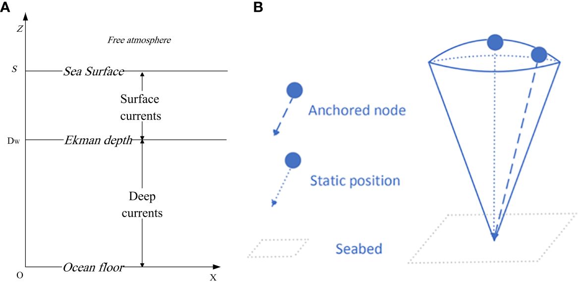
Figure 1 (A) Ocean current model. (B) Mobile nodes.
Ekman current is the surface current that develops from wind at the ocean surface (Cushman Roisin and Beckers, 2011). As wind blows over the ocean, a surface current develops due to the drag at the wind water interface. As shown in Figure 2A, the X axis corresponds to the east, the Y axis corresponds to the north, and the Z axis corresponds to the vertical direction. In the Northern Hemisphere, the surface current of ocean water moves at 45° to the right of the wind. As shown in Figure 2A, the wind direction is north, and the ocean surface current direction at 45° to the right of north.

Figure 2 (A) Ekman current model. (B) Velocity and direction of each successive layer.
If the ocean is divided vertically into thin layers, each successive layer moves more toward the right and at a slower speed. The total depth of the frictional influence of the wind is called the Ekman depth. Ekman transport is a net transport of the water between the ocean surface and Ekman depth, and Ekman transport is at 90° to the right of the wind in the northern hemisphere.
In this paper, the ocean below the Ekman depth belongs to the deep current. As shown in Figure 2B, the deep ocean flows westward, opposite to the Ekman transport direction. The current velocity between depth Dw and depth T increases uniformly from 0 to a fixed-value velocity deep, and the velocity from depth T to the seabed is fixed at velocity deep.
Similar to the panda hunter model commonly used in SLP on land, the roles and features of each node need to be clarified before we integrate SLP into UASNs. The attacker waits the signals coming from the UASNs that begin near the sink node and performs a backtracking attack. Although the goal of the attacker is the location information of DAQ that deployed on the seabed, we do not treat DAQ as the source nodes. In this model, it is assumed that once the attacker finds the AUV, they can obtain the position of all DAQ by following the AUV. Therefore, the AUV is treated as the source node, and the following assumptions were made:
1. Sink node: The sink node is located on the ocean surface, and the number of sink node is at least one. The sink node can communicate with the datacenter on the shore and exchange data packets with UASNs.
2. UASN: All sensor nodes are homogeneous in the UASN. Each sensor node has the same computing power, storage space, battery power, and so on. Each node is affected simultaneously by the pull of anchored wire, buoyancy force, and wallop of the water current. As shown in Figure 1B, every node offset around their static positions and move noticeably within a spherical crown surface (Liu et al., 2012).
3. Source node: Each AUV is a source node, and at least one source node exists in the model. An AUV is an unmanned, untethered vehicle used to conduct underwater research. They are able to move faster and quietly, collecting data from DAQs by using a scheme and so on (Che and Yu, 2020; Lv et al., 2020; Ojha et al., 2020; Zeng et al., 2020). However, the details of the DAQs data collected by an AUV are beyond the scope of this article.
4. DAQs: DAQs measure real-world physical conditions and convert samples into digital numeric values. The details of the data collected by DAQs are beyond the scope of this article.
The purpose of an adversary is to find the location of the source node. In this study, the features of the adversary are assumed as follows:
1. There is only one adversary in the network. Their equipment has powerful computing power, big storage space, and sufficient power. It is assumed that the adversary will not miss the nearby packets. The adversary can solve the tracking control problem according to the information of the direction and velocity of the ocean currents.
2. The adversary performs passive attacks and find the source location by backtracking the traffic flow. To be more precise, the adversary never attacks the node or damage the network topology and communication. We assumed that the adversary knows nothing about the packet contents.
3. The adversary is a local attacker, which means that the monitoring range of the adversary is limited due to the effect of currents, noise interference, and high transmission delay. In this model, the monitoring range was the same as the communication range of the nodes in UASN, and the adversary will not miss any nearby data packets.
4. When the adversary performs a backtracking attack and arrives at a new location, he will wait for the arrival of a new signal if the source node is not found yet. If no new signal comes for a long time, the adversary will return to the last position and repeat the backtracking attack.
In the ConeSLP scheme, there are four types of nodes: sink, UASN, AUV, and DAQ. The AUV gathers data from DAQs and transmit the data to sink by using UASN. In order to realize ConeSLP, our research focused on the detail of the following aspects:
1. Since ocean currents change the location of sensor nodes, we must first determine how nodes are deployed in the UASN. A good deployment method helps to improve the success rate of the routing algorithm to generate the communication path.
2. Even if there is interference from ocean currents, the routing method used by UASN can dynamically plan a communication path to realize the communication between sink and AUV. This routing method should enhance the UASN’s ability to defend against backtracking attacks, thereby safeguarding the SLP of the network.
3. The routing algorithm not only prevents an adversary from locating the AUV through a backtracking attack but also allows the AUV to easily contact the UASN.
At the beginning, the number of nodes owned by UASN is node_n, and all the nodes are randomly distributed in a circular area with radius circle_r on the seabed. Each node floats at different ocean depths by changing the length of the anchored wire, and the distribution at this time is called the initial state. In the initial state, all the nodes are distributed on the side of a cone with height cone_h and radius circle_r. As shown in Figure 3A, node_n = 600, circle_r = 300, cone_h = 800, and each red dot means a position of a node on the seabed, while the blue dots mean the initial state.
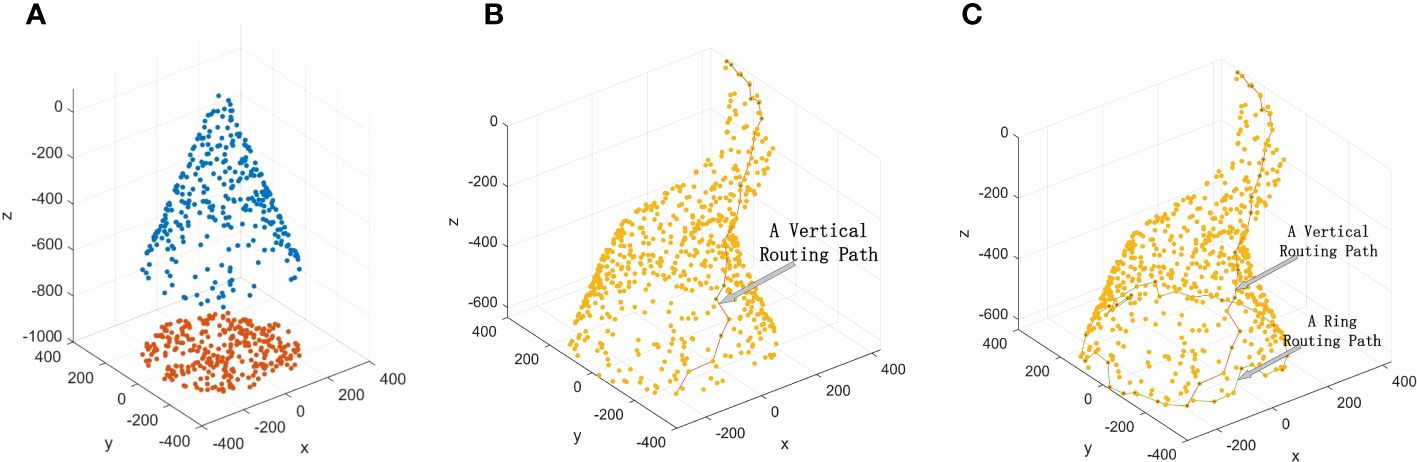
Figure 3 (A) Initial state of UASN. (B) Vertical routing path. (C) Circular routing path.
In order to balance the energy consumption and security performance, the UASN routing path consists of two parts: a routing path and a circular routing path. As shown in Figure 3B, the vertical routing path ensures that the packets can reach the deep ocean from the ocean surface. As shown in Figure 3C, the circular routing path increases the complexity of the routing path to strengthen the safety performance of the path. In addition, the AUV can flexibly select one node in the circular routing path to exchange packets.
The nodes used to build the routing path remain active, and the remaining nodes in the UASN sleep until the next routing, which can extend the lifetime of the UASN.
The sensor nodes owned by UASN are randomly distributed on the seabed. AUV assists these nodes to locate themselves and gives them the center coordinate and radius of the circle which includes all nodes. As shown in Figure 4A, three nodes are distributed in circle O, the center of circle O is (0, 0, 1,000), the radius = circle_r, and each node reaches the initial state by changing the length of the anchored wire.
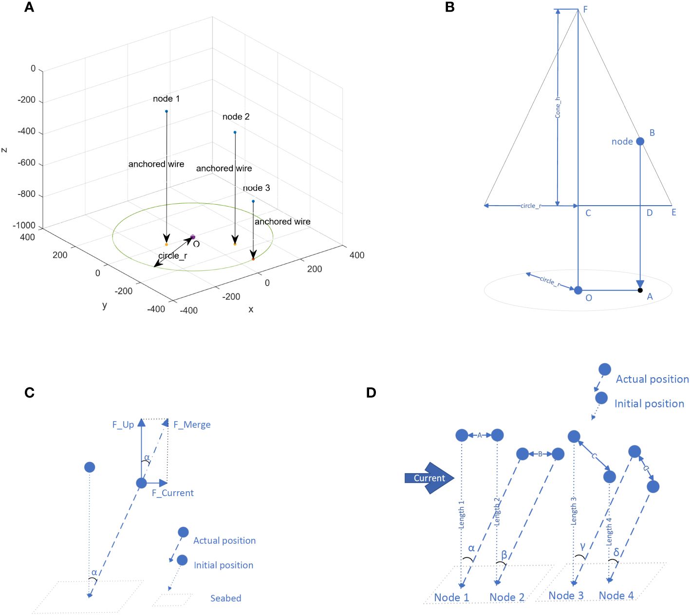
Figure 4 (A) The initial state. (B) Calculate the wire length. (C) Calculate α. (D) Connectivity between two nodes.
Each node can obtain the values of cone_h and circle_r from the AUV, and the length of its own anchored wire (wire_length) can be calculated as shown in Figure 4B.
Based on Equations 1-5, wire_length can be derived as shown in Equation 6. lAO is the distance between the anchor point of node and the point O, and lAD is the distance between the cone and the seabed.
Distributing the nodes on the side of a cone can bring some benefits as follows:
1. As shown in Figures 3A, B, because of the symmetry of the cone, regardless of the changes in the direction and speed of ocean currents, we can use the same set of algorithm to plan routing paths, which effectively simplifies the algorithm.
2. It is very convenient to adjust the parameters of the cone, such as changing the cone_h, which can be achieved by updating the length of anchored wire according to the new cone_h. Each node can independently adjust its own anchored wire length to update the UASN topology.
3. When there are ocean currents, the connectivity of UASN may not necessarily decrease and may even increase.
Calculating the effect of ocean currents on the position of nodes is beyond the scope of this article. This research uses some generally accepted formulas for experiments.
As shown in Figure 4C, the force applied to node is divided into two directions, horizontal (F_Current) and vertical (F_Up), and the combined force determines the value of R.
F_Up equal to the buoyancy of the node minus the gravity, which can be considered a fixed value. In this article, it is assumed that F_Current is composed of fluid drag (F_Drag) and viscosity resistance (F_Resistance), as shown in Equations 7-9.
The velocity of ocean currents is relatively slow, so we assume that F_Drag and F_Resistance change approximately linearly and get Equation 10.
At this point, we can use Equation 11 to calculate α.
When K = is set, Equation 12 is generated.
When ocean current exists, the connectivity of UASN may not be decreased and may even be increased. As shown in Figure 4D, the anchored wire of node 1 and node 2 are the same. In the same ocean current, α = β, so the distance between them in the initial position (A) and actual position (B) are equal. In other words, distance A = distance B. Compared with the initial state, the connectivity between the two nodes in the ocean current has not changed. The anchored wire length of node 4 is shorter than that of node 3. Although γ = δ is derived from Equation 12, distance C > distance D, which means that the connectivity between the two nodes in the current is optimized compared to the initial state.
We distribute the sensors on the side surface of a cone. Because of the symmetry of the cone, the connectivity of the sensors on the side close to the ocean current is guaranteed.
In the UASN, the vertical routing path is a transmission path for packets from the cone top to the bottom, and the path is constructed by UASN nodes. The vertical routing path is affected by ocean currents and spontaneously and dynamically by the UASN nodes. A good vertical path has at least two features, namely:
1. Through the vertical routing path, packets can be quickly transmitted between the ocean surface and the deep.
2. The path can prevent attacks from carrying out backtracking attacks.
In this research, two vertical routing methods are provided. Method 1 is based on the depth of the nodes, and Method 2 focuses on the parameters of the Ekman current in addition to the depth of the nodes. The advantage of Method 1 is that the path is constructed with as few nodes as possible, so the transmission of the packet is fast. In Method 2, the connectivity between nodes is better, and the safety performance of the path is good.
• Method 1: based on the depth of the nodes.
In UASN, some sensors near the ocean surface can directly communicate with the sink, and one of these sensors is selected as the first node of the vertical routing path. Algorithm 1 illustrates the process of generating the first node of the path.
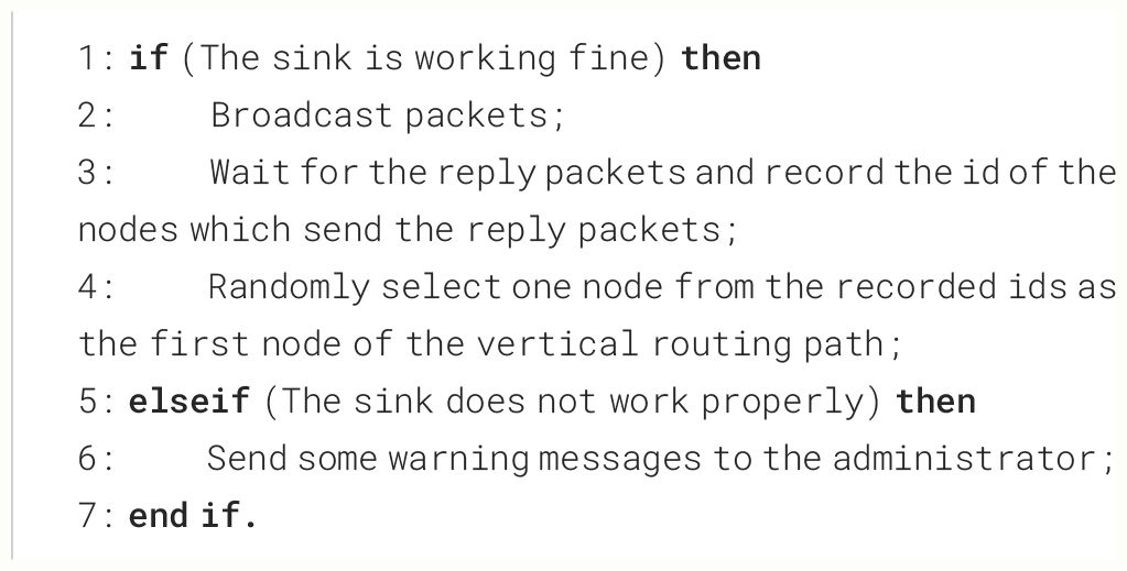
Algorithm 1. The birth of the first node of the vertical routing path.
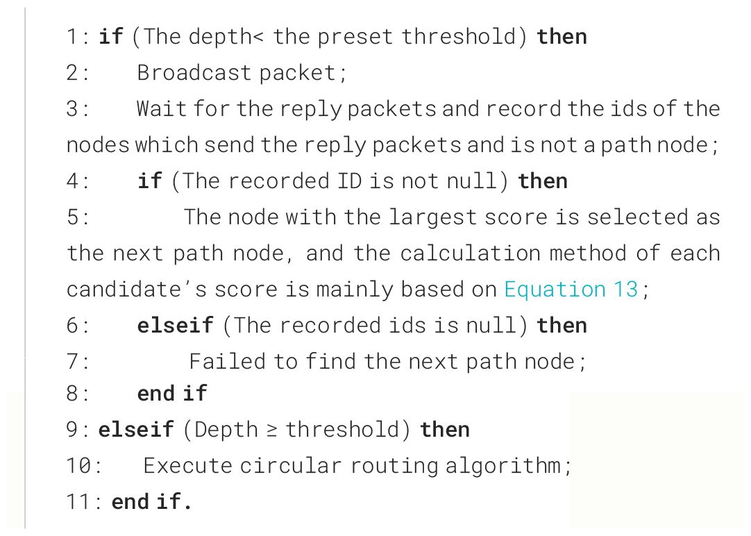
Each path node takes all nodes in its communication range as the candidates, and the algorithm used to find the next path node from these candidates is intuitive, as shown in Algorithm 2.
The path node performs different operations according to its own depth. If the depth is smaller than the preset threshold, Algorithm 2 is used to find the next vertical path node; otherwise the circular routing algorithm is executed.

Algorithm 2. The way to find the next path node: Method 1.
As shown in Figure 5, node F is the path node selected by node C, and F gets its next path node according to Algorithm 2. There are five neighbor nodes within the communication range of F, but there are only four candidate nodes—namely, D, E, G, and H. Node C is not a candidate node because it is already a path node. Among all the candidate nodes, H has the largest depth; so, H is the next path node selected by F.
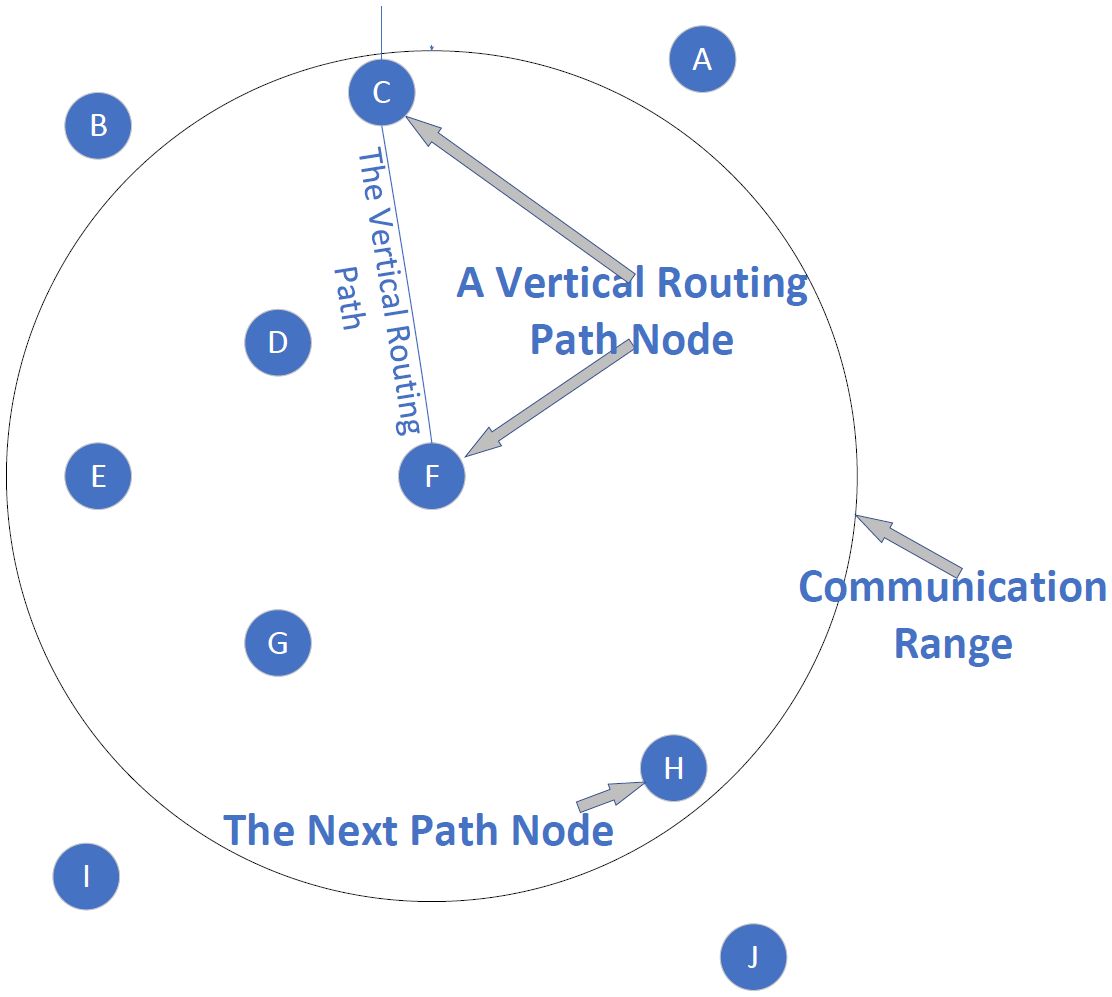
Figure 5 Example of using Method 1 to find the next path node.
In Figure 6, the right part shows a vertical routing path obtained by using Method 1, and the left part adds the display of nodes.
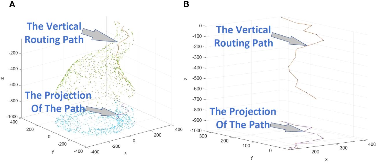
Figure 6 (A) Example of a vertical path obtained by using Method 1, displaying nodes. (B) Example of a vertical path obtained by using Method 1, excluding nodes.
• Method 2: based on the parameters of the Ekman current
In Method 2, considering the influence of the characteristics of the Ekman current, Algorithm 3 is used by each path node to select the next path node. Figure 7A is the initial state of 300 randomly distributed nodes. Considering the influence of ocean currents, the distribution is shown in Figure 7B.
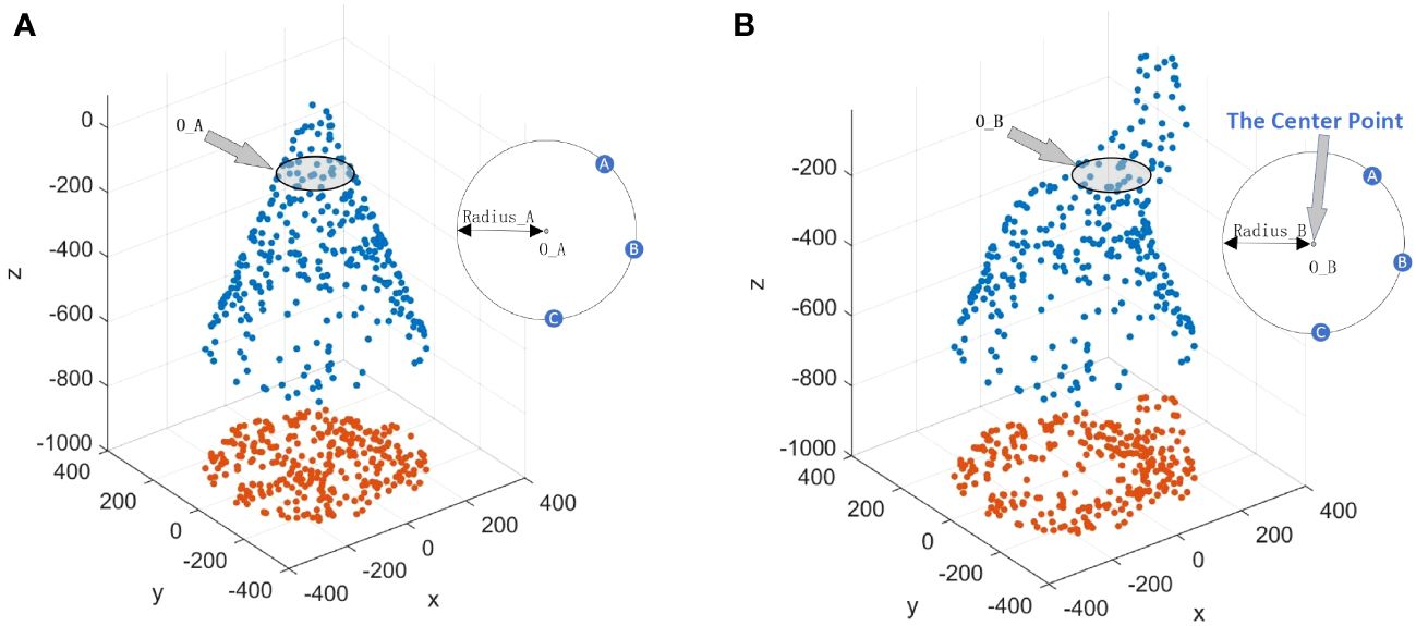
Figure 7 (A) Circle O_A cuts the cone into two parts. (B) Circle O_B cuts the cone into two parts.
Suppose there is a circle named O_A parallel to the sea lever and O_A cuts the cone into two parts, as shown in Figure 7A. Then, O_A will move to the new position named O_B under the influence of ocean current, as shown in Figure 7B. The radius of the two circles will not change, so Radius_A = Radius_B. In addition, the relative position between the nodes on the circle and the center of the circle will not change. The only difference between the two circles is their depth. Circle O_A is closer to the ocean surface than circle O_B. In Figure 7B, point OB is the center of the circle O_B, and nodes A, B, and C are on the circle. In order to describe Method 2 more conveniently, point O_B is named as “the center point” of nodes A, B, and C. In the following, we will continue to use the phrase “the center point”.
According to the Ekman current model, the Dw (Ekman depth) can be calculated (Cushman Roisin and Beckers, 2011). If the depth increases by 1 m, the ocean current direction changes 180 ÷ Dw degrees.
In Figure 8A, node B looks for the next path node. Node B will evaluate each candidate node and give a score, and the node with the largest score is the next path node. We take the process of calculating the score of node C as an example to illustrate the details. Node B is a path node, and point O is the center point of B. Line_O is a line perpendicular to the sea level, passing through point O. Plane_B is a plane passing through Line_O and node B, and Plane_C is passing through Line_O and node C. α is the angle between Plane_B and Plane_C.
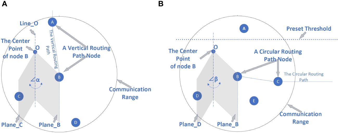
Figure 8 (A) Example of using Method 2 to find the next path node. (B) Example of finding the next circular routing path node.
The score of each candidate node is calculated using Equation 13. Take node C as an example; Depth is the depth of node C, and α is the angle between planes B and Plane C. Degree can be calculated by using Equation 14. X and Y are two variables, and they can be adjusted as needed.
In Equation 14, DepthPathNode is the depth of the path node, which is equivalent to the depth of node B in Figure 8A. Dw is Ekman depth; the ocean current direction changes 180 ÷ Dw degrees as the current depth increases by 1 m.
When the environment such as the ocean current features changes, we will update the X and Y in Equation 13. If necessary, we can even completely change the equation. However, it needs to be emphasized that, in methods, the purpose of using Equation 13 is to take the current features into consideration when selecting path nodes.
Figure 9B shows the vertical routing path obtained by using Method 2, and Figure 9A adds the display of nodes.
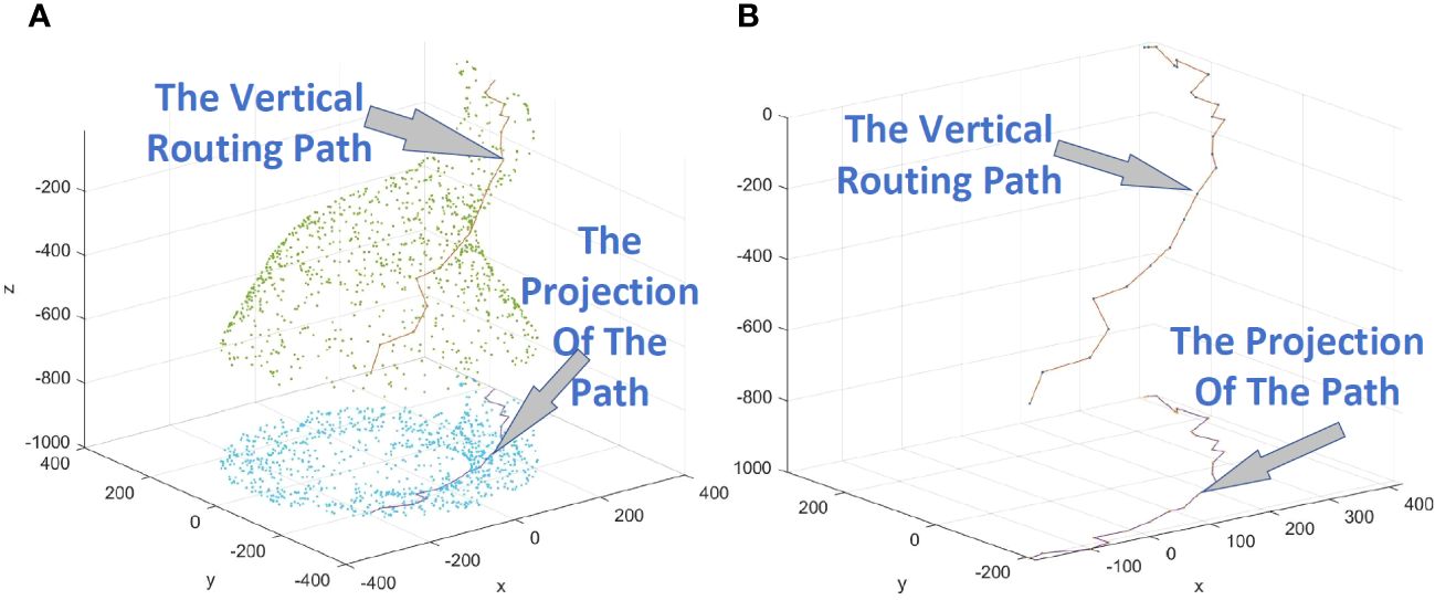
Figure 9 (A) Example of a vertical path obtained by using Method 2, displaying the nodes. (B) Example of a vertical path obtained by using Method 2, with the nodes no longer displayed.
Algorithm 3. The way to find the next path node: Method 2.
There is a preset threshold in the ConeSLP scheme, which is a number smaller than the depth of the cone’s bottom. If the depth of a path node is bigger than the threshold, the path node is the last node of the vertical routing path. The last node of the vertical routing path is the first node of the circular routing path.
The circular routing path is a circular path, connected end to end. Each path node divides the nodes within the communication range into two categories. The nodes whose depth are greater than A belong to the first category, and the remaining nodes belong to the second category. The path node takes the first category’s nodes as candidates and then calculates the score of each candidate according to Equation 15. The node with the highest score is the next path node.
In Equation 15, Depth is the depth of the candidate. β is the angle between Plane_B and Plane_D, as shown in Figure 8B. U and V are two variables, and they can be adjusted as needed.
In Figure 8B, node B looks for the next path node. Node B will evaluate each candidate node and give a score, and the node with largest score is the next path node. We take the process of calculating the score of node D as an example to illustrate the details. There are four neighbor nodes within the communication range of B, but there are only two candidate nodes, namely, D and E. Node C is not a candidate node because it is already a path node, and node A is not a candidate because its depth is smaller than the preset threshold. Among all the candidate nodes, D has the largest depth, so D is the next path node selected by B. Algorithm 4 is used to find the next circular path node.
Figure 10B shows a circular routing path, and Figure 10A adds the display of nodes.
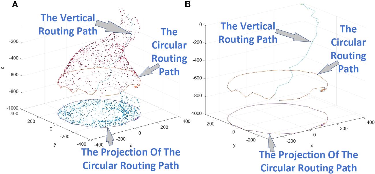
Figure 10 (A) Example of a circular routing path, displaying the nodes. (B) Example of a circular routing path, with the nodes no longer displayed.
The communication path of UASN is composed of two parts, including the vertical routing path and the circular routing path. The last node of the circular routing path will send a “hello packet” to its previous path node. The “hello packet” is passed to the previous path node by each path node until it reaches the sink. Then, the sink will broadcast ‘“sleep packet” to notify all nodes to sleep except for the path nodes, and the specific time for sleep is notified in the “sleep packet”.

Algorithm 4. The way to find the next circular routing path node.
The AUV can collect ocean current information and analyze the approximate location of the cone’s bottom. The AUV sails along the cone’s bottom and periodically sends a “request” packet. If a ring node responds to the AUV’s request, it will send a “response” packet. Then, AUV and UASN get in touch, and data can be transferred.
As shown in Figure 11, the AUV receives the “response” packet from node C and starts to transmit data with C. The path required for these data includes two parts: the path between BC and the path between AB. The path between BC belongs to the circular routing path, and the path between AB belongs to the vertical routing path.
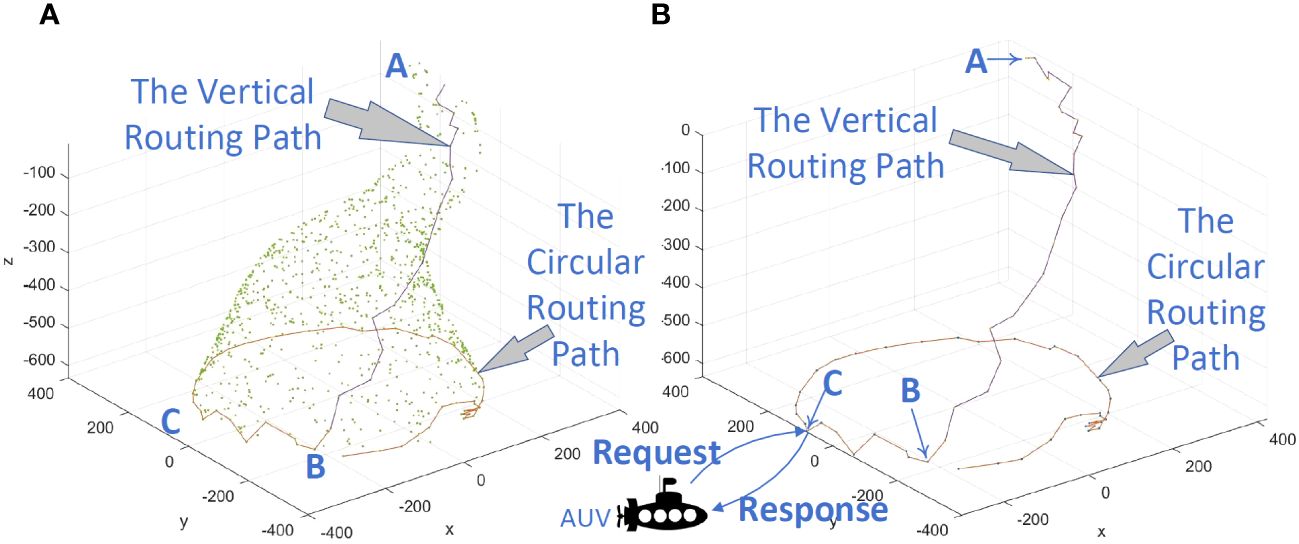
Figure 11 (A) Communication between AUV and UASN, displaying the nodes. (B) Communication between AUV and UASN, with the nodes no longer displayed.
The attacker tracks the traffic flow in the vertical routing path and reaches the circular routing path—for example, in Figure 11, the attacker arrives at point B from point A according to the backtracking attack. When the attacker continues to reach point C by tracking the traffic flow, the AUV may have already left. Assuming that the sum of the lengths of path AB and path BC is LengthAC, then LengthAC is the shortest distance that the attacker needs to travel to find the AUV.
If we disguise the AUV as a ring node, the attacker will travel a greater distance but cannot be sure of finding the AUV. In Figure 12, the AUV gets in touch with node B, and the AUV temporarily replaces node B. Node D pretends to be an AUV and generates false data packets to transmit in the circular routing path.
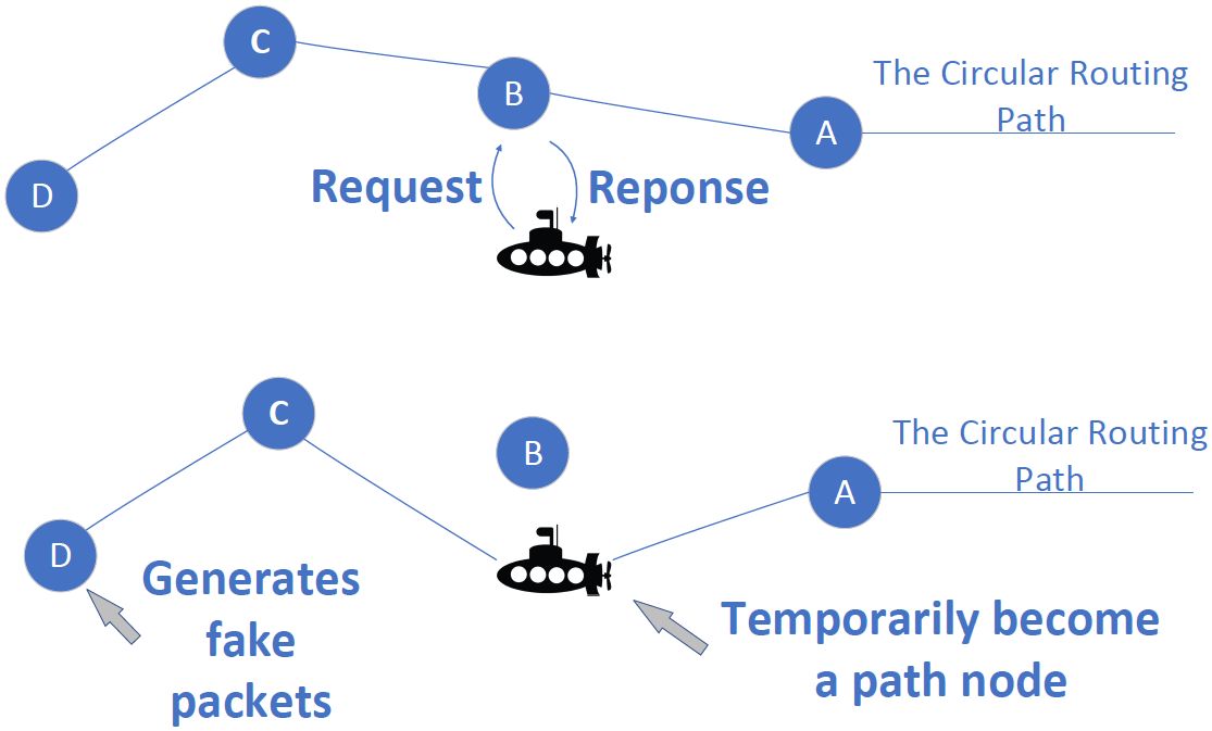
Figure 12 The AUV temporarily becomes a path node.
In this study, we adopted three commonly analyzed SLP metrics: safety distance, energy consumption, and connectivity. We cannot show all the experimental results in this paper, so these metrics were evaluated under four simulation conditions: the velocity of the ocean current on the ocean surface, the number of underwater sensor nodes, the communication range, and the height of the cone.
The safety distance refers to the length of the vertical path and the length of the loop path. The sum of the two lengths is the maximum distance that an attacker needs to travel to find the AUV, and the length of the vertical path is the minimum distance that the attacker needs to travel to find the AUV. Energy consumption refers to the energy consumption required by the path to transmit a data packet. Connectivity mainly refers to the proportion of the UASN in successfully constructing a routing path under different metrics settings.
The simulation was conducted in MATLAB R2018a, and the underwater sensor nodes of UASN are all the same. Few researchers have considered SLP in UASNs; therefore, we selected two coverage schemes for water environment as comparison algorithms to show the importance and necessity of researching location privacy in UASN.
Before presenting the performance of the ConeSLP scheme, we first show the weakness (Wang W et al., 2019; Chang et al., 2019). Similar to the common UASN routing scheme, these two schemes are area coverage methods and not suitable for the network model in this research. The more nodes that can communicate directly with the sink node, the longer the lifetime of a UASN. This is because in a UASN, the nodes near the base station consume the most energy. As shown in Figure 13, ConeSLP scheme deploys nodes in a cone, and the schemes deploy nodes in a cylinder (Wang et al., 2019; Chang et al., 2019). The cone and the cylinder have the same height and radius, and the number of nodes deployed is the same. The network areas covered within the communication radius of the sink node are areas 1 and 2, respectively. In Figure 14A, the height of the cone and the cylinder is 800 m, the radius of the bottom surface is 300 m, and there are 1,000 nodes. In Figure 14B, the radius is changed to 500 m, and the rest of the metrics remain unchanged. In Figure 14A, when the communication radius expands to 150 or more, the number of nodes in area 2 exceeds that of area 1. As the radius of the cone and cylinder increases, as shown in Figure 14B, the number of nodes in area 1 is always greater than that in area 2. This shows that the larger the radius, the more the advantages of ConeSLP. In contrast, our proposed ConeSLP scheme takes SLP into consideration, and the lifetime of the network is longer than these previously proposed schemes.
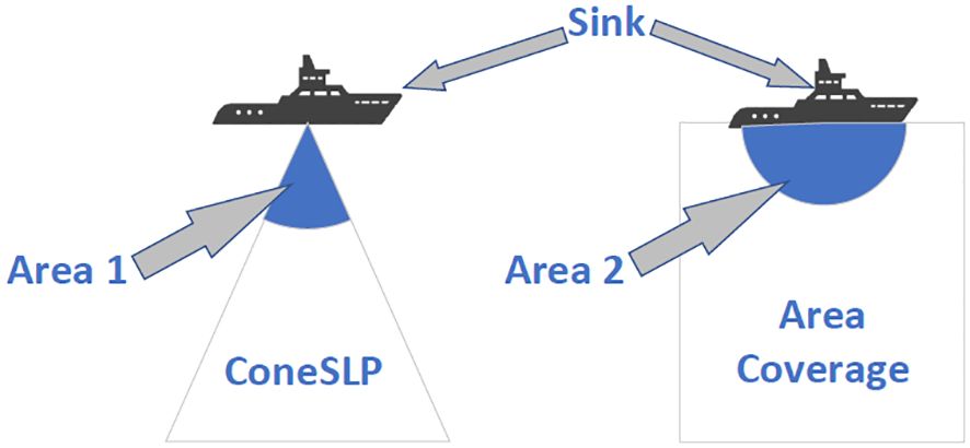
Figure 13 Number of nodes close to the sink.
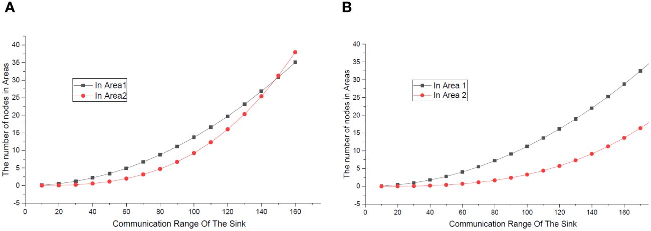
Figure 14 (A) Number of nodes in areas, A; the radius is 300. (B) Number of nodes in areas, A; the radius is 500.
The attack eavesdrops the traffic flow to find the source location. The safety distance was the distance traveled by the adversary to find the location of the source. In other words, when the attack moves to the AUV, SLP is broken. Thus, the longer the safety distance, the safer the network. In this research, SLP protection in the underwater environment was judged based on the moving distance of the attacker; the distance is bigger than the length of the routing path that consists of the vertical routing path and the circular routing path.
We conducted three sets of experiments with the main metrics settings shown in Table 1. Each set of experiment is divided into two groups that use the same circular routing method, but the vertical routing methods are Method 1 and Method 2. In Figure 15, when Method 1 is used, the length of the vertical routing path is “Method 1: V”, the length of the circular routing path is “Method 1: C”, and the length of the total routing path is “Method 1: V+C”. When using Method 2, the routing path lengths are represented similarly.
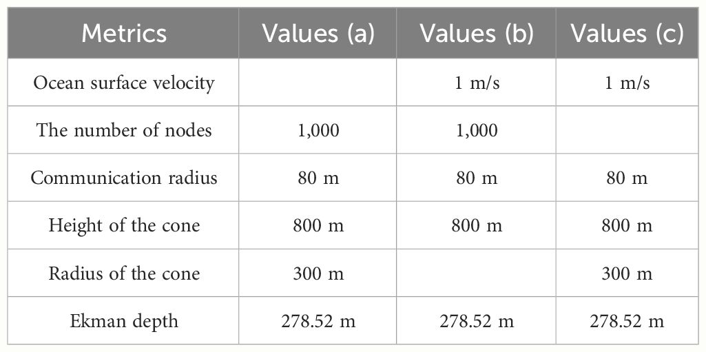
Table 1 Metrics settings for safety distance and energy consumption experiments.
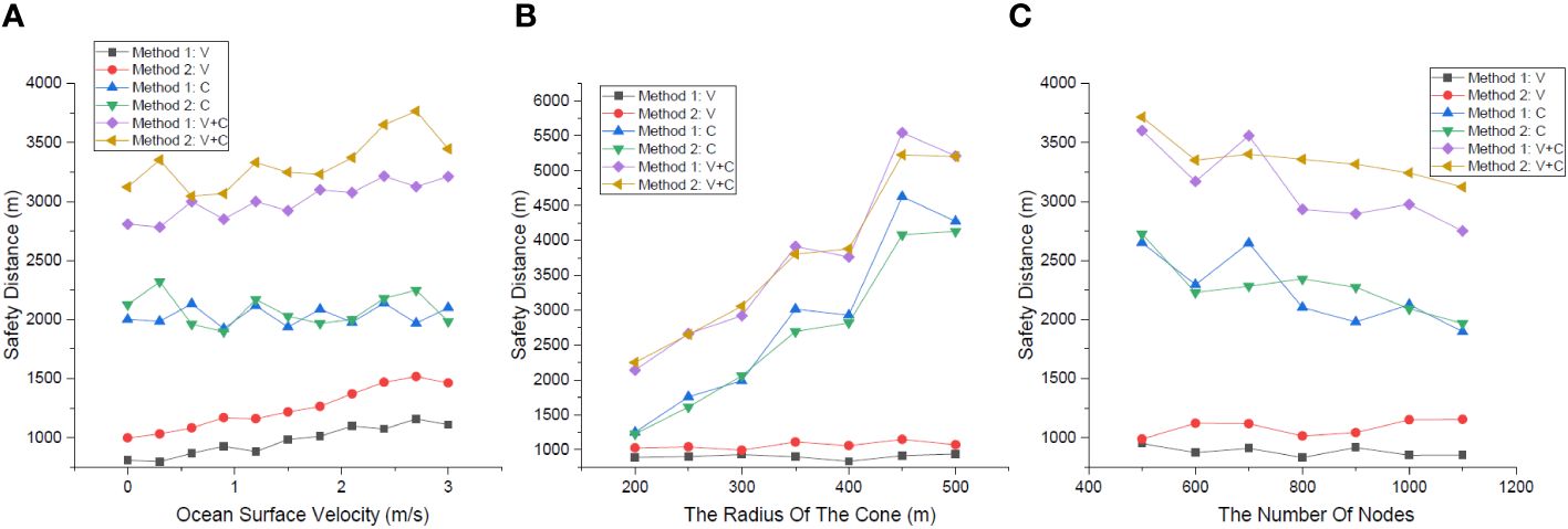
Figure 15 (A) Safety distance at different values of ocean surface velocity. (B) Safety distance at different radius measurements. (C) Safety distance at different number of nodes.
The relationship between safety distance and the ocean surface velocity is shown in Figure 15A, in which the metrics are settled as “Values (a)” in Table 1. The ocean surface velocity ranges from 0 to 3 m/s. In general, the vertical routing path length increases with velocity, and the length of the circular routing path remains stable. The increasing value of velocity makes the effect of the Ekman layer on the nodes distribution more pronounced, and the vertical routing path length difference between Method 2 and Method 1 becomes larger. This is due to the increased ocean surface velocity, which results in an increased distance between the nodes in the surface and deep currents. When considering the ocean surface velocity, the safety distance of Method 2 is always larger than that of Method 1.
The relationship between the safety distance and the cone’s radius is shown in Figure 15B, in which the metrics are settled as “Values (b)” in Table 1. The cone’s radius ranges from 200 to 500 m. Because the cone’s height is fixed, the values of “Method 1: V” and “Method 2: V” do not fluctuate much, and “Method 1: V” is smaller than “Method 2: V”. As the radius increases, the values of “Method 1: C” and ‘“Method 2: C” both increases, but the magnitude of both values are uncertain. This is because each path is planned in a new distribution of nodes, where the nodes are randomly distributed.
The relationship between the safety distance and the number of underwater sensor nodes is shown in Figure 15C, in which the metrics are settled as “Values (c)” in Table 1. The number of nodes ranges from 500 to 1,100 m. Most notably, when the number of nodes increases, each routing path node has more candidates for the next hop within its communication range, and the ConeSLP scheme may attempt to construct the shortest circular routing path. As a result, the more nodes in the network, the smaller the length of the circular routing path. The values of “Method 1: V” and “Method 2: V” do not fluctuate much, and “Method 1: V” is smaller than “Method 2: V” always. Owing to the random distribution of nodes, the circular routing path length of Method 1 is larger than that of Method 2 when the number of nodes is 700. In general, “Method 2: V+C” is bigger than “Method 1: V+C” always. This means that using Method 2 in the ConeSLP scheme yields a better safety distance than using Method 1.
Energy consumption means the energy consumption of the routing path nodes in this paper. The energy consumption of the node was calculated following the method (Wang et al., 2016). We conducted three sets of experiments with main metrics settings as shown in Table 1. Each set of experiment is divided into two groups that use the same circular routing method, but the vertical routing methods are Method 1 and Method 2. All the experiments’ results are shown in Figure 16A. The relationship between the average energy consumption of the routing path nodes and the ocean surface velocity is presented in Figure 16A.a. When the velocity increases, the overall trend shows that “Method 2: V+C” is bigger than “Method 1: V+C”. This is because “Method 2: V” is bigger than “Method 1: V”. ConeSLP can get a better safety distance using Method 2 than using Method 1, but at the cost of a higher energy consumption.
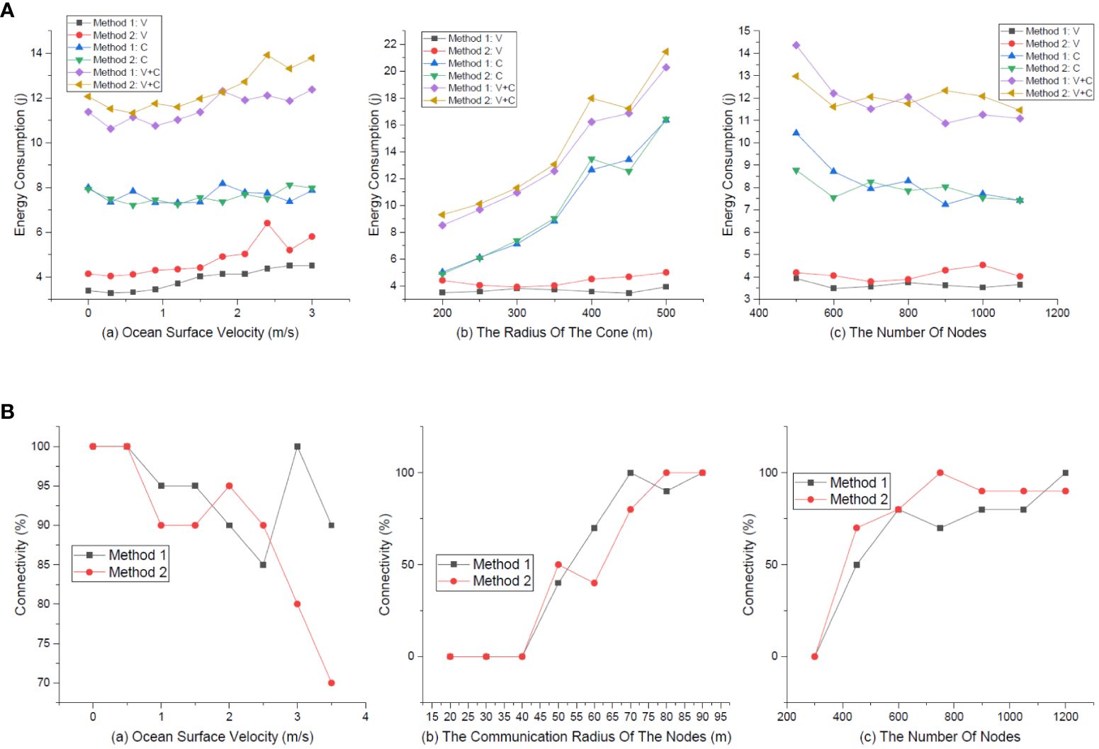
Figure 16 (A) Energy consumption. (B) Connectivity.
The relationship between energy consumption and cone’s radius is shown in Figure 16A.b, and Figure 16A.c shows the relationship between energy consumption and the number of nodes. In summary, similar to the result in (a), “Method 2: V+C” is mostly larger than “Method 1: V+C” in Figures 16A.b and Figures 16A.c. This is because “Method 1: C” and “Method 2:C” have similar values, and the values of “Method 1: V” are smaller than those of “Method 2: V”. In other words, using Method 2 in the ConeSLP scheme yields a better safety distance than using Method 1. The cost of having a larger safety distance is higher energy consumption. If we want to reduce the energy consumption, we can deploy more nodes in the USAN or reduce the cone’s radius.
Connectivity mainly refers to the proportion of the UASN successfully constructing a routing path under different metrics settings. We conducted three sets of experiments with main metrics settings as shown in Table 2. Each set of experiment is divided into two groups that use the same circular routing method, but the vertical routing methods are Method 1 and Method 2. Owing to experimental error and the random distribution of nodes in each independent experiment, the lines in the figure were not very smooth but still available for observing trends in connectivity.
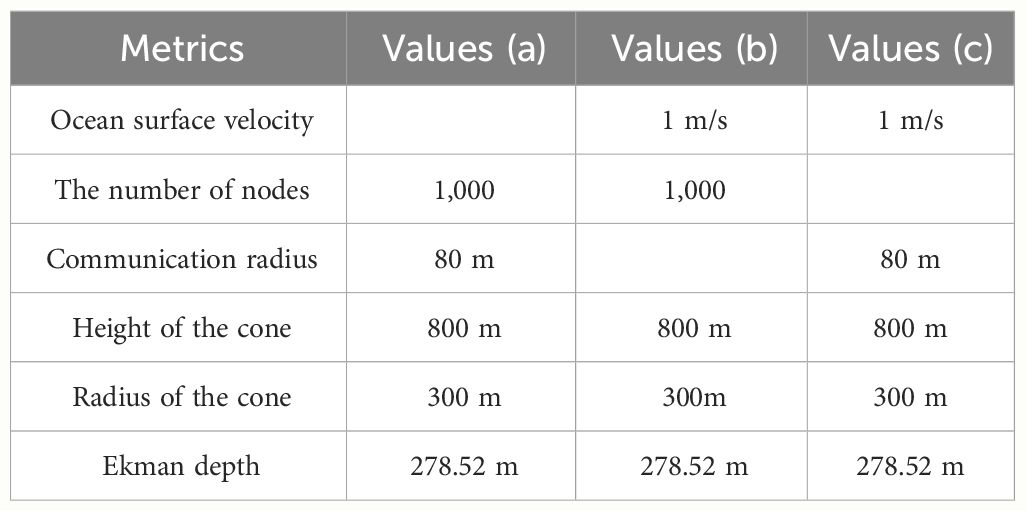
Table 2 Metrics settings for connectivity experiments.
The relationship between the connectivity and the ocean surface velocity is shown in Figure 16B.a, in which the metrics are settled as “Values (a)” in Table 2. Unlike Method 1, Method 2 generates a vertical routing path that takes Ekman layer into account. We expected ConeSLP with Method 2 to have better connectivity at any ocean surface velocity than with Method 1, but the experiments provide different results than expected. We first discuss the connectivity of ConeSLP using Method 1 at a different ocean surface velocity. For ease of exposition, we refer to the connectivity rate of ConeSLP using Method 1 as the connectivity of Method 1. The connectivity of Method 1 decreases continuously when the ocean surface velocity ranges from 0 to 2.5 m/s. This is consistent with common sense. Whereas at the ocean surface velocity in the range of 2.5 to 3 m/s there is an increase in Method 1’s connectivity because the cone undergoes severe deformation and nodes on one side of the cone are able to communicate directly with nodes on the other side, as the ocean surface velocity increases and further cone deformation occur, the connectivity of Method 1 decreases dramatically. We next discuss the connectivity of Method 2 at a different ocean surface velocity. The connectivity of Method 2 maintains a decreasing trend when the ocean surface velocity ranges from 0 to 1.5 m/s. When the range of the velocity is from 1.5 to 2, the connectivity of Method 2 increases, and the scheme gets good results by considering Ekman layer factors; in other words, Equation 13 gets better results under the value of current ocean surface velocity. When the ocean surface velocity is bigger than 2 m/s, the connectivity of Method 2 decreases rapidly. It should be noted that when the ocean surface velocity is at 3.5 m/s, the connectivity of Method 2 is significantly lower than Method 1. There are at least two reasons: first, compared with Method 1, Method 2 constructs a vertical routing path that requires more path nodes, which reduces the connectivity; and second, when the cone is severely deformed, the parameters of Equation 13 are not adjusted.
The relationship between the connectivity and the communication of the nodes is shown in Figure 16B.b, in which the metrics are settled as “Values (b)” in Table 2. When the communication radius of the nodes is less than 40 m, the routing path cannot be successfully constructed, and the connectivity of both Method 1 and Method 2 is zero. As the communication radius gradually increases, the connectivity of both increases. When the communication radius is 50 and 80 m, the connectivity of Method 1 is smaller than Method 2. Other than that, the connectivity of Method 1 is close to or bigger than Method 2. This is because Method 2 builds a vertical routing path over longer distances and uses more nodes than Method 1 always. In general, the larger the communication radius of the nodes, the bigger the connectivity of both Method 1 and Method 2.
The relationship between the connectivity and the number of nodes in UASN is shown in Figure 16B.c, in which the metrics are settled as “Values (c)” in Table 2. When the number of nodes in the UASN gradually increases from 300 to 1,000, Method 2 has a higher connectivity than Method 1; such experimental results also show that Method 2 is meaningful. Method 2 has a longer routing path than Method 1,and whether it has a higher connectivity depends on whether the parameters of Equation 13 are set to accommodate UASN’s deployment environment.
Protecting the security and privacy of UASNs is an important research area, especially in 3d ocean monitoring field. In this paper, we have proposed a new scheme called ConeSLP to incorporate source location privacy into UASNs. The Ekman current and deep current were employed to simulate the underwater environment. The routing paths generated by ConeSLP scheme include a vertical routing path and a circular routing path, and we provide two methods to generate the vertical path and one method to generate the vertical paths. The two vertical routing-path-generation algorithms are named Method 1 and Method 2, respectively. Method 1 generates a routing path based on the depth of the nodes. Both Method 2 and the circular-routing-path-generating algorithm select routing path nodes based on equations designed with Ekman’s properties in mind. ConeSLP using Method 2 will typically have a greater safety distance than using Method 1, but at the cost of a higher energy consumption. Whether the ConeSLP using Method 2 will have better connectivity than using Method 1 depends on whether the equations are properly parameterized or not. Currently, parameter setting is done empirically, and much work remains to be done to automate parameter setting for specific underwater environment. Furthermore, we are currently focused on source location privacy protection of UASNs under passive attacks and will be working on active attacks in the future.
The original contributions presented in the study are included in the article/supplementary material. Further inquiries can be directed to the corresponding author.
PJ: Conceptualization, Data curation, Formal analysis, Methodology, Software, Validation, Writing – original draft, Writing – review & editing. HW: Conceptualization, Funding acquisition, Methodology, Validation, Writing – review & editing. ZX: Data curation, Software, Writing – review & editing.
The author(s) declare financial support was received for the research, authorship, and/or publication of this article. This work was partly supported by Zhejiang Province Philosophy and Social Science Planning Project (20NDJC344YBM), The National Natural Science Foundation of China (No. 62102132), and The National Vocational Education Teachers' Teaching Innovation Team Research Project (No. YB2021010103).
The authors declare that the research was conducted in the absence of any commercial or financial relationships that could be construed as a potential conflict of interest.
All claims expressed in this article are solely those of the authors and do not necessarily represent those of their affiliated organizations, or those of the publisher, the editors and the reviewers. Any product that may be evaluated in this article, or claim that may be made by its manufacturer, is not guaranteed or endorsed by the publisher.
AlMistarihi M. F., Tanash I. M., Yaseen F. S., Darabkh K. A. (2020). Protecting source location privacy in a clustered wireless sensor networks against local eavesdroppers. Mobile Networks Appl. 25, 42–54. doi: 10.1007/s11036-018-1189-6
Bradbury M., Jhumka A. (2017). “A near optimal source location privacy scheme for wireless sensor networks,” in 2017 IEEE Trustcom/BigDataSE/ICESS. IEEE, 409–416. doi: 10.1109/Trustcom/BigDataSE/ICESS.2017.265
Cebeci T., Shao J. P., Kafyeke F., Laurendeau E. (2005). Computational fluid dynamics for engineers from panel to navier-stokes methods with computer programs 2005. Eng. Educ. System 41, 603–605. doi: 10.1007/3–540-27717-X
Chang J., Shen X., Bai W., Zhao R., Zhang B. (2019). Hierarchy graph based barrier coverage strategy with a minimum number of sensors for underwater sensor networks. Sensors 19, 2546. doi: 10.3390/s19112546
Che G., Yu Z. (2020). Neural network estimators based fault tolerant tracking control for AUV via ADP with rudders faults and ocean current disturbance. Neuro computing. 411, 442–454. doi: 10.1016/j.neucom.2020.06.026
Cushman Roisin B., Beckers J. M. (2011). “The ekman layer,” in In International Geophysics. 101, 239–270. doi: 10.1016/B978–0-12–088759–0.00008–0
Dutta N., Saxena A., Chellappan S. (2010). “Defending wireless sensor networks against adversarial localization,” in 2010 eleventh international conference on mobile data management. 336–341.
Gao S., Cheng S., Jin Q., Li SC., Jin H., Wang S., et al. (2023). Model test research of wave induced submarine landslide based on Fibre Bragg Grating sensing technology. Ocean Eng. 291, 15. doi: 10.1016/j.oceaneng.2023.116492
Hao Z., Qu N., Dang X., Hou J. (2019). RSS based coverage deployment method under probability model in 3D-WSN. IEEE Access 7, 183091–183104. doi: 10.1109/Access.6287639
Kamarei M., Patooghy A., Alsharif A., Hakami V. (2020). SiMple: A unified single and multi-path routing algorithm forWireless sensor networksWith source location privacy. IEEE Access 8, 33818–33829. doi: 10.1109/Access.6287639
Kirton J., Bradbury M., Jhumka A. (2018). Towards optimal source location privacy aware TDMA schedules in wireless sensor networks. Comput. Networks 146, 125–137. doi: 10.1016/j.comnet.2018.09.010
Liu L., Wang R., Xiao F. (2012). Topology control algorithm for underwater wireless sensor networks using GPS free mobile sensor nodes. J. Network Comput. Appl. 35, 1953–1963. doi: 10.1016/j.jnca.2012.07.017
Lv P. F., He B., Guo J., Shen Y., Yan T. H., Sha Q. X. (2020). Underwater navigation methodology based on intelligent velocity model for standard AUV. Ocean Eng. 202, 107073. doi: 10.1016/j.oceaneng.2020.107073
Münchow A., Schaffer J., Kanzow T. (2020). Ocean circulation connecting fram strait to glaciers off Northeast Greenland: mean flows, topographic rossby waves, and their forcing. J. Phys. Oceanography 50, 509–530. doi: 10.1175/JPO-D-19-0085.1
Mutalemwa L. C., Shin S. (2019). Regulating the packet transmission cost of source location privacy routing schemes in event monitoring wireless networks. IEEE Access 7, 140169–140181. doi: 10.1109/Access.6287639
Mutalemwa L. C., Shin S. (2020). Secure routing protocols for source node privacy protection in multi-hop communication wireless networks. Energies 13, 292. doi: 10.3390/en13020292
Ojha T., Misra S., Obaidat M. S. (2020). SEAL: Self-adaptive AUV based localization for sparsely deployed Underwater Sensor Networks. Comput. Commun. 2020, 204–215. doi: 10.1016/j.comcom.2020.02.050
Ozturk C., Zhang Y., Trappe W. (2004). “Source location privacy in energy constrained sensor network routing,” in Proceedings of the 2nd ACM workshop on Security of ad hoc and sensor networks SASN ‘04, Washington DC, USA (ACM Press), 88–93. doi: 10.1145/1029102.1029117
Ponni R., Jayasankar T., Kumar K. V. (2023). Investigations on underwater acoustic sensor networks framework for RLS enabled loRa networks in disaster management applications. J. Of Inf. Sci. Engineering. 39(2), 389–406.
Song X., Gong Y., Jin D., Li Q. (2019). Nodes deployment optimization algorithm based on improved evidence theory of underwater wireless sensor networks. Photonic Network Commun. 37, 224–232. doi: 10.1007/s11107-018-0807-3
Sun W. Y., Sun O. M. (2020). Inertia and diurnal oscillations of Ekman layers in atmosphere and ocean. Dynamics Atmospheres Oceans 2020, 101144. doi: 10.1016/j.dynatmoce.2020.101144
Wang W. P., Chen L., Wang J. X. (2008). “A source location privacy protocol in WSN based on locational angle,” in 2008 IEEE International Conference on Communications. 1, 1630–1634. doi: 10.1109/ICC.2008.315
Wang Q., Dai H. N., Li X., Wang H., Xiao H. (2016). On modeling eavesdropping attacks in underwater acoustic sensor networks. Sensors 16, 16. doi: 10.3390/s16050721
Wang H., Han G., Lai W., Hou Y., Lin C. (2023). A multi round game based source location privacy protection scheme with AUV enabled in underwater acoustic sensor networks. IEEE Trans. Vehicular Technol. 72, 7728–7742. doi: 10.1109/TVT.2023.3237653
Wang W., Huang H., He F., Xiao F., Jiang X., Sha C. (2019). An enhanced virtual force algorithm for diverse k-coverage deployment of 3D underwater wireless sensor networks. Sensors 19, 3496. doi: 10.3390/s19163496
Wang Y., Liu L., Gao W. (2019). An efficient source location privacy protection algorithm based on circular trap for wireless sensor networks. Symmetry 11, 632. doi: 10.3390/sym11050632
Yao L., Kang L., Deng F., Deng J., Wu G. (2015). Protecting source location privacy based on multi-rings in wireless sensor networks: PROTECTING SOURCE LOCATION PRIVACY. Concurrency Computation: Pract. Exp. 27, 3863–3876. doi: 10.1002/cpe.3075
Zeng Z., Zhou H., Lian L. (2020). Exploiting Ocean energy for improved AUV persistent presence: path planning based on spatio temporal current forecasts. J. Mar. Sci. Technol. 2020, 26–47. doi: 10.1007/s00773-019-00629-0
Keywords: submarine disaster, dynamic routing, source location privacy, underwater acoustic sensor network, Ekman currents
Citation: Jiang P, Wang H and Xiong Z (2024) A dynamic routing scheme for underwater acoustic sensor networks in submarine disaster applications. Front. Mar. Sci. 11:1400586. doi: 10.3389/fmars.2024.1400586
Received: 18 March 2024; Accepted: 02 May 2024;
Published: 07 June 2024.
Edited by:
Chuan Lin, Northeastern University, ChinaReviewed by:
Loong Xiaohan, Changzhou College of Information Technology, ChinaCopyright © 2024 Jiang, Wang and Xiong. This is an open-access article distributed under the terms of the Creative Commons Attribution License (CC BY). The use, distribution or reproduction in other forums is permitted, provided the original author(s) and the copyright owner(s) are credited and that the original publication in this journal is cited, in accordance with accepted academic practice. No use, distribution or reproduction is permitted which does not comply with these terms.
*Correspondence: Hao Wang, d2FuZ2hhb2hodUBvdXRsb29rLmNvbQ==
Disclaimer: All claims expressed in this article are solely those of the authors and do not necessarily represent those of their affiliated organizations, or those of the publisher, the editors and the reviewers. Any product that may be evaluated in this article or claim that may be made by its manufacturer is not guaranteed or endorsed by the publisher.
Research integrity at Frontiers
Learn more about the work of our research integrity team to safeguard the quality of each article we publish.