A TMSBL underwater acoustic channel estimation method based on dictionary learning denoising

The shallow sea underwater acoustic channel exhibits a significant sparse multipath structure. The temporally multiple sparse Bayesian learning (TMSBL) algorithm can effectively estimate this sparse multipath channel. However, the complexity of the algorithm is high, the signal-to-noise ratio (SNR) of shallow-sea underwater acoustic communication is low, and the estimation performance of the TMSBL algorithm is greatly affected by noise. To address this problem, an improved TMSBL underwater acoustic channel estimation method based on a dictionary learning noise reduction algorithm is proposed. Firstly, the K-Singular Value Decomposition (K-SVD) dictionary learning method is used to reduce the noise of the received pilot matrix, reducing the influence of noise on the signal. Then, the Generalized Orthogonal Matching Pursuit (GOMP) channel estimation method is combined to obtain a priori information such as the perceptual matrix and hyperparameter matrix for TMSBL channel estimation; and the noise variance is obtained by using the null subcarrier calculation instead of iteratively updating the noise variance in the TMSBL, to improve the estimation accuracy and reduce the algorithmic complexity. Finally, the TMSBL channel estimation method is used to estimate the underwater acoustic channels of different symbols jointly. The simulation results show that the normalized mean square error of the channel estimation of the improved TMSBL method is reduced by about 92.2% compared with the TMSBL algorithm, obtaining higher estimation accuracy; running time is reduced by about 45.6%, and there is also better performance in terms of the running speed, which provides a reference for underwater acoustic channel estimation.

1 Introduction

Underwater acoustic communication is a crucial means of transmitting information in the ocean due to its high reliability and data transmission rates (Xu et al., 2016; Xing et al., 2021b; Zhang et al., 2021; Zhang et al., 2024). The use of Orthogonal Frequency Division Multiplexing (OFDM) technology is widespread in high-speed underwater acoustic communication due to its effectiveness against frequency-selective fading, efficient band utilization, robust resistance to multipath propagation, and straightforward implementation of channel equalization (Jia et al., 2022). The underwater acoustic channel is considered one of the most complex channels due to its multipath, time-varying, frequency-varying, and null-varying characteristics (Xing et al., 2022; Xing et al., 2023). In the underwater acoustic channel of shallow seas, reflections and scattering from the seafloor and sea surface cause significant delay extension and multipath effects. These effects result in a sparse multipath structure at the receiving end (Tong et al., 2022; Yang, 2023; Zhang, 2023). The multipath structure is formed at the receiving end. The shallow sea underwater acoustic channel’s complex and variable nature significantly impacts the OFDM communication system (Yin et al., 2021). To ensure communication quality, it is necessary to estimate the channel state at the receiving end. The key characteristic parameters obtained through channel estimation are used to adjust the signal processing method, which serves as a crucial basis for achieving channel matching and improving the quality of signal recovery. This is of great importance in improving the performance of underwater acoustic OFDM communications in shallow sea environments.

The underwater acoustic channel exhibits significant sparse characteristics. However, traditional channel estimation algorithms, such as Least Square (LS) and Minimum Mean Square Error (MMSE), fail to leverage the sparsity of the underwater acoustic channel, necessitating a large number of pilot signals for accurate channel estimation, resulting in serious occupation of spectral resources (Meng and Liu, 2023). To achieve accurate channel estimation that exploits the sparsity of the channel, compressed sensing techniques are employed for sparse channel estimation with a large number of zero taps in the time domain response (Wu and Tong, 2017; Jiang et al., 2021; Meng and Liu, 2023). Matching Pursuit (MP) is a greedy iterative algorithm widely employed in compressed sensing for sparse channel estimation. It exhibits higher estimation accuracy compared to methods such as LS and MMSE (Cotter and Rao, 2002). Another category of compressed sensing reconstruction algorithms, including Least Absolute Shrinkage And Selection Operator (LASSO) (Tibshirani, 1996) and Basis Pursuit (BP) (Chen et al., 2001), constitutes convex optimization tracking algorithms grounded in paradigm constraints. They seek the approximation of sparse signals by converting a non-convex problem into a solvable convex problem. These algorithms, in comparison with traditional methods, harness the sparse characteristics of the underwater acoustic channel, leading to higher estimation accuracy. However, their performance is significantly influenced by sparsity selection, and their computational complexity is high, rendering practical applications challenging. To enhance the channel estimation technique, we leverage the priori knowledge of the sparse signal. Introducing the sparse Bayesian learning class algorithm, based on the Bayesian criterion, into the sparse channel estimation problem (Chen et al., 2020; Lyu et al., 2021) yields improved estimation performance and has been extensively researched.

Algorithms for sparse signal reconstruction using sparse Bayesian learning have been extensively researched in recent years (Wipf and Rao, 2004; Wipf and Rao, 2007; Zhang and Rao, 2011). Wipf and Rao, 2004 (Wipf and Rao, 2004) introduced the Sparse Bayesian Learning (SBL) algorithm for sparse signal reconstruction in single-measurement models; Subsequently, in 2007 (Wipf and Rao, 2007), they extended it to multi-measurement models and derived the Multiple Sparse Bayesian Learning (MSBL) algorithm for sparse signal reconstruction. In (Zhang and Rao, 2011) the Temporal Sparse Bayesian Learning (TSBL) algorithm and its extension, the TMSBL algorithm based on the MSBL algorithm, are derived. Among these algorithms, the TMSBL algorithm not only leverages the channel sparsity property but also explores the correlation between channels. It considers the priori distribution of the channel and incorporates space-time information, resulting in high channel estimation accuracy. Consequently, the TMSBL algorithm has found widespread use in underwater channel estimation (Qiao et al., 2018; Hong et al., 2022). Consequently, the TMSBL algorithm finds extensive application in underwater channel estimation. In (Qiao et al., 2018), the TMSBL algorithm is incorporated into the channel estimation of slow time-varying underwater acoustic OFDM communication systems. Correlation is utilized to jointly estimate the channels of several consecutive blocks. This approach achieves optimal performance in strongly time-correlated channels and maintains robustness in weakly time-correlated channels. However, it is more sensitive to noise, which leads to degraded estimation accuracy and increased computational complexity in low signal-to-noise ratio scenarios. In (Hong et al., 2022), singular value decomposition noise reduction is performed to address the above challenges. Using LS channel estimation to obtain a priori information such as perception matrix and hyperparameter matrix of TMSBL for high-precision and low-complexity underwater acoustic OFDM communication. However, due to the increased noise sensitivity of the LS channel estimation method and the limited effectiveness of the singular value decomposition for noise reduction, the accuracy of the channel estimation is reduced under low signal-to-noise ratio conditions.

Dictionary learning algorithms provide effective noise reduction and are widely used in image denoising, active sonar target classification, and weak signal detection in underwater acoustic (Wang et al., [[NoYear]]; Zhu et al., 2020; Xing et al., 2021a). It is common for existing channel estimation methods to incorrectly identify noise as channel tap coefficients in environments with a low signal-to-noise ratio (SNR). This reduces the accuracy of channel estimation and increases the computational complexity. To address the limitations of the previously mentioned channel estimation methods and to account for the sparse multipath structure of the signal in the shallow sea underwater acoustic channel, we utilize the dictionary learning algorithm for TMSBL underwater acoustic channel estimation. As a result, we propose an enhanced TMSBL underwater acoustic channel estimation method based on the dictionary learning noise reduction algorithm. Initially, the enhanced K-SVD dictionary learning algorithm is employed to reduce the noise of the received pilot matrix, thereby enhancing the accuracy of channel estimation under low signal-to-noise ratio conditions. Subsequently, the initialization parameter matrix and perception matrix of TMSBL are acquired by integrating the GOMP channel estimation method. This integration alleviates the limitation of the TMSBL method, where noise is erroneously estimated as a channel tapping coefficient. Lastly, the null subcarrier of the OFDM system is utilized to obtain a more precise noise variance, replacing the step of updating the noise variance in TMSBL. This modification reduces the complexity of the TMSBL algorithm and enhances estimation accuracy. The paper’s contributions can be summarized as follows.

1. The K-SVD dictionary learning algorithm is employed in the domain of underwater acoustic communication to denoise the received signal pilot matrix, thereby mitigating the impact of noise on channel estimation accuracy and enhancing the performance of underwater acoustic OFDM communication systems.

2. The GOMP channel estimation method is employed to derive the time-domain underwater acoustic channel impulse response and the initialization and perception matrices for the TMSBL algorithm, thereby reducing the number of iterations and the computational complexity of the TMSBL algorithm. Furthermore, the incorporation of the priori knowledge addresses the limitation of the TMSBL method, which is prone to misestimating noise as a channel tap coefficient. This enhances the overall performance of channel estimation.

The rest of the article is organized as follows. In Section 2, the received signal model and the TMSBL channel estimation method are introduced. Section 3 presents enhanced TMSBL channel estimation methodologies, including a K-SVD dictionary learning-based noise reduction technique and a method for obtaining TMSBL priori knowledge using the GOMP algorithm. The efficacy of the proposed algorithm is substantiated through simulations in Section 4. Further validation of the algorithm using sea trial experimental data is provided in Section 5, demonstrating its effectiveness in real marine environments. The paper concludes in Section 6.

2 TMSBL-based underwater acoustic channel estimation method

2.1 Received signal model

In underwater acoustic communications in shallow seas, signal propagation is significantly affected by reflections, diffraction, and scattering from both the sea surface and seafloor. This results in a complex multipath structure of the underwater acoustic channel. The underwater acoustic channel exhibits a significant sparse characteristic due to signal energy absorption by seawater during most of the multipath propagation. The mathematical expression for the channel impact response of the underwater acoustic time-varying channel is given by (Cheng and Wang, 2022).

$\begin{array}{ll}\begin{array}{c}h(t,\tau )={\displaystyle \sum _{i=1}^L}{h}_i(t)\delta (\tau -{\tau }_i(t))\end{array}& (1)\end{array}$

where $h(t)$ is the channel impulse response at time t, and L is the multipath number, the $h_i(t)$ and ${\tau }_i(t)$ are denoted as the gain and delay of the ith path at time t, respectively.

Consider an OFDM system with N subcarriers, L pilots, and channel coherence time significantly exceeding the OFDM symbol period. If the impulse response of the channel remains time-invariant within one OFDM symbol period, (Equation 1) can be expressed as follows:

$\begin{array}{ll}\begin{array}{c}h(\tau )={\displaystyle \sum _{i=1}^L}{h}_i\delta (\tau -{\tau }_i)\end{array}& (2)\end{array}$

Assuming the cyclic prefix of OFDM symbols exceeds the maximum multipath delay of the channel, the frequency domain expression for the OFDM communication system is:

$\begin{array}{ll}\begin{array}{c}\mathit{y}=\mathit{X}\mathit{F}\mathit{h}+\mathit{v}\end{array}& (3)\end{array}$

where $\mathit{y}\in {ℂ}^{N\times 1}$ is the received signal, $\mathit{X}\in {ℂ}^{N\times N}$ is the diagonalization matrix with diagonal elements representing the transmitted signals. $\mathit{F}\in {ℂ}^{N\times M}$ is the DFT matrix, and $\mathit{h}\in {ℂ}^{M\times 1}$ is the time domain channel impulse response. The v follows $\mathcal{C}\mathcal{N}(0,\lambda {\mathit{{\rm I}}}_N)$ of Gaussian white noise. From the received signal y out of the pilot signal, the received model of the pilot signal is:

$\begin{array}{ll}\begin{array}{c}{\mathit{y}}_p={\mathit{X}}_p{\mathit{F}}_p\mathit{h}+{\mathit{v}}_p\end{array}& (4)\end{array}$

where ${\mathit{y}}_p\in {ℂ}^{p\times 1}$ is the received pilot signal, ${\mathit{X}}_p\in {ℂ}^{p\times p}$ is the diagonalization matrix with diagonal elements representing the known pilot signals. ${\mathit{F}}_p\in {ℂ}^{p\times M}$ is the corresponding DFT matrix at the pilot position. The system model described in (Equation 4) is a single-measurement model. A multi-measurement model is considered: several different OFDM symbols are modeled with the following expressions:

$\begin{array}{ll}\begin{array}{c}{\mathit{Y}}_p={\mathit{X}}_p{\mathit{F}}_p\mathit{H}+{\mathit{V}}_p={\mathit{\Phi }}_p\mathit{H}+{\mathit{V}}_p\end{array}& (5)\end{array}$

Among them. ${\mathit{Y}}_p=[{\mathit{y}}_{p,1},{\mathit{y}}_{p,2},\dots ,{\mathit{y}}_{p,L}]\in {ℂ}^{p\times L}$ represents the received pilot matrix of L OFDM symbols, and ${\mathit{\Phi }}_{\mathit{p}}\in {ℂ}^{p\times M}$ is the perception matrix, $\mathit{H}=[{\mathit{h}}_1,{\mathit{h}}_2,\dots ,{\mathit{h}}_L]\in {ℂ}^{M\times L}$.

2.2 TMSBL underwater acoustic channel estimation

The article uses the TMSBL algorithm (Qiao et al., 2018), using temporal correlation to jointly estimate (Equation 5) of H the estimation reconstruction problem. Firstly, the priori probability of each H_i is modeled as:

$\begin{array}{ll}\begin{array}{c}p({\mathit{H}}_i;{\gamma }_i,{\mathit{B}}_i)~N(0,{\gamma }_i{\mathit{B}}_i), i=1,\dots ,M\end{array}& (6)\end{array}$

where H_i is the ith row of H, i.e., the number of channels tapping coefficients for different OFDM symbols at the same moment; γ_i is the nonnegative hyperparameter matrix that controls the sparsity of each row in H. When ${\gamma }_i=0$, ${\mathit{H}}_i=0$; B_i is a positive definite matrix, which represents the temporal correlation structure among the elements within H_i and can be estimated using the TMSBL algorithm for the positive definite matrix B. (Equation 6) can be written as:

$\begin{array}{ll}\begin{array}{c}p({\mathit{H}}_i;\mathit{\Gamma },{\mathit{B}}_i)={\displaystyle \prod _{i=1}^M}p({\mathit{H}}_i;{\gamma }_i,{\mathit{B}}_i)\end{array}& (7)\end{array}$

where Γ is the hyperparameter matrix $\mathit{\Gamma }=\text{diag}(\mathit{\gamma })=\text{diag}({[{\gamma }_1,{\gamma }_2,\dots ,{\gamma }_M]}^T)$.

H_i, Obeying the mean Gaussian probability distribution, its posterior probability can be written as:

$\begin{array}{ll}\begin{array}{c}p({\mathit{h}}_l|{\mathit{y}}_{p,l};\mathit{\Gamma })\sim N({\mathit{\mu }}_l,\mathit{\Sigma }), l=1,2,\dots ,L\end{array}& (8)\end{array}$

where the mean and covariance can be expressed as:

$\begin{array}{ll}\begin{array}{c}\mathit{\sum }=({\text{σ}}^{-2}{\Phi }_p^{\text{H}}{\Phi }_p+{\Gamma }^{(r)}-1){-}^1\end{array}& (9)\end{array}$

$\begin{array}{ll}\begin{array}{c}\mathit{M}=[{\mathit{\mu }}_1,{\mathit{\mu }}_2,\dots ,{\mathit{\mu }}_L]={\text{σ}}^{-2}\Sigma {\Phi }_p^{\text{H}}{\mathit{Y}}_p\end{array}& (10)\end{array}$

Of these, μ_l and $\mathit{ℳ}$ are respectively the estimated values of H_i and H. ${\Gamma }^{(r)}$ is the estimated value of the Γ update matrix for the first r iteration of the Expectation Maximization (EM) algorithm. The hyperparameters are estimated using the EM algorithm. The E-step update rule of the EM algorithm is given in (Equations 9, 10). The M-step update rule is given in:

$\begin{array}{ll}\begin{array}{c}{\mathit{\gamma }}_i=\frac{1}{L}{\mathit{ℳ}}_i{B}^{-1}{\mathit{ℳ}}_i^{\text{H}}+{\displaystyle \mathit{\sum }(i,i)}\end{array}& (11)\end{array}$

$\begin{array}{ll}\begin{array}{c}\mathit{B}=(\frac{1}{M}{\displaystyle \sum _{i=1}^M}\frac{\Sigma (\mathit{\text{i}},\mathit{\text{i}})}{{\gamma }_i})\mathit{B}+\frac{1}{M}{\displaystyle \sum _{i=1}^M}\frac{H_i^{\text{H}}{\mathit{H}}_i}{{\gamma }_i}\end{array}& (12)\end{array}$

$\begin{array}{ll}\begin{array}{c}{\sigma }^2=\frac{1}{pL}\Vert {\mathit{Y}}_p-{\mathit{\Phi }}_p\mathit{H}{\Vert }_F^2+\frac{{\sigma }^2}{p}Tr({\mathit{\Phi }}_p\mathit{\Gamma }{\mathit{\Phi }}_p^{\text{H}}({\sigma }^2\mathit{I}+{\mathit{\Phi }}_p\mathit{\Gamma }{\mathit{\Phi }}_p^{\text{H}})-1)\end{array}& (13)\end{array}$

where ${\Vert \cdot \Vert }_F^2$ denotes the quadratic of the F-parameter of the vector $Tr(\cdot )$ is the trace of the matrix. The joint estimation of the channel impulse response after the iteration of the EM algorithm is completed $\widehat{\mathit{H}}=\mathit{ℳ}$.

(Equation 13) is the updated formula for the noise variance, which is calculated using the null subcarriers of the OFDM system:

$\begin{array}{ll}\begin{array}{c}{\sigma }^2=E[{\left|{\mathit{Y}}_n\right|}^2]\end{array}& (14)\end{array}$

where Y_n is the frequency domain null subcarrier. Using (Equation 14) to obtain a more accurate noise variance, a more accurate channel estimation can be obtained. This reduces the influence of the noise variance by the TMSBL input parameters such as the number of iterations, the threshold, and the received frequency-conducting matrix. At the same time, it can reduce the TMSBL algorithm for the σ² update step in the TMSBL algorithm, reducing the complexity of the algorithm.

3 Improved TMSBL channel estimation method

The conventional TMSBL channel estimation method is susceptible to misidentifying noise as channel tapping coefficients in low SNR conditions of underwater acoustic channels, resulting in reduced channel estimation accuracy. Simultaneously, the increase in channel length leads to heightened computational complexity. Furthermore, the TMSBL algorithm inadequately utilizes the characteristics of the underwater acoustic channel for selecting the initial parameters of the EM algorithm, leading to excessive iterations and slower convergence in computation.

Aiming at the limitations of the traditional TMSBL algorithm, the K-SVD dictionary learning algorithm is used on the receiver side to perform noise reduction and reconstruction of the received pilot matrix Y_p, and obtains the noise-reduced receiver pilot matrix ${\mathit{Y}}_p^{\text{'}}$, enhancing channel estimation accuracy under low SNR conditions. Following this, the GOMP algorithm is utilized to estimate the underwater acoustic channel, acquiring a priori knowledge for the TMSBL algorithm. This knowledge involves removing invalid atoms and smaller hyperparameters from the dictionary. Finally, the TMSBL algorithm, combined with the a priori knowledge from the GOMP algorithm, conducts joint channel estimation for different OFDM symbols. The block diagram of the receiver system based on the improved TMSBL channel estimation method is depicted in Figure 1.

Figure 1

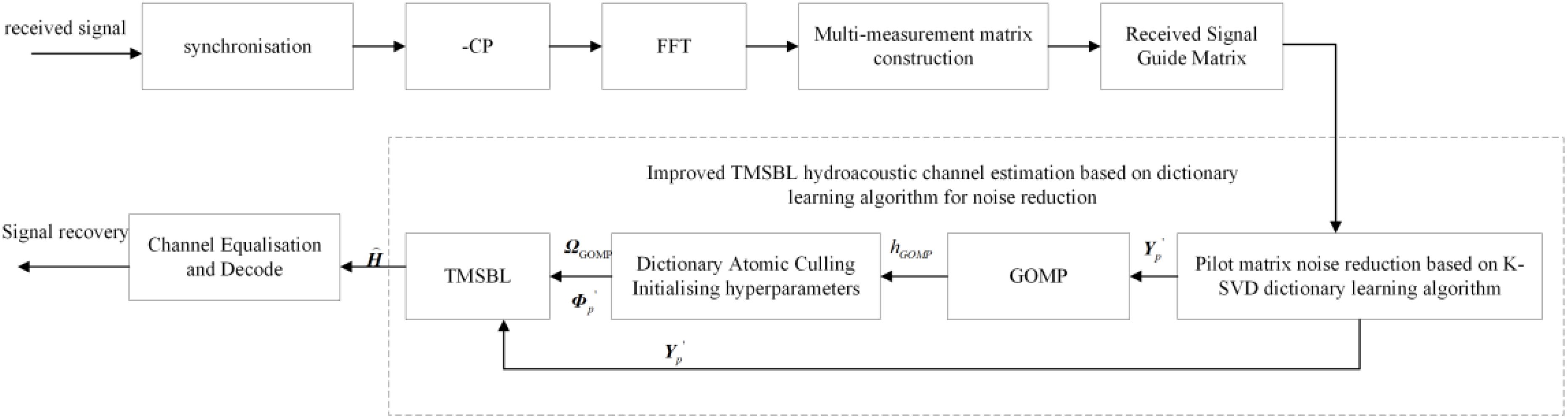
Figure 1. Block diagram of the receiver system based on the improved TMSBL channel estimation method.

3.1 K-SVD-based noise reduction of the received pilot matrix

According to the theory of sparse decomposition, Y_p can be decomposed into ${\mathit{Y}}_p={\mathit{X}}_p{\mathit{F}}_p\mathit{H}+{\mathit{V}}_p=\mathit{A}({\mathit{X}}_s+{\mathit{X}}_n)$. Where $\mathit{A}\in {ℂ}^{p\times J}$ is the redundant dictionary matrix, X_s and X_n are the sparse coefficient matrices corresponding to ${\mathit{X}}_p{\mathit{F}}_p\mathit{H}$ and V_p, respectively. As the signal is sparse, whereas the noise is not sparse, and the coefficient values are generally very small, existing only in a finite number of non-zero coefficients, the approximated signal obtained by the linear combination of these sparse counterparts of the atoms contains the vast majority of the information about the signal, while the vast majority of the noise is discarded, thus realizing the purpose of noise cancellation. Let $\mathit{X}={\mathit{X}}_s+{\mathit{X}}_n$, then ${\mathit{Y}}_p=\mathit{A}\mathit{X}$. Where $\mathit{X}\in {ℂ}^{J\times L}$ is the sparse coefficient matrix. To achieve the sparse decomposition of the signal, a suitable dictionary needs to be constructed. The dictionary learning algorithm is employed to construct a suitable redundant dictionary to enhance signal reconstruction.

The K-SVD dictionary learning algorithm is a new dictionary learning algorithm proposed by Aharon and Elad et al (Aharon et al., 2006). The primary concept behind the K-SVD algorithm involves updating a set of atoms in the dictionary along with their sparse coefficients simultaneously. Through iterations of updating a set of atoms within the dictionary, if, when updating any atom, the remaining atoms remain unchanged, the dictionary is then updated with the sparse coefficients. a_i with no change in the remaining atoms, the a_i new sparse coefficients will be obtained after the update X_i. When the error reaches the threshold, the whole dictionary post-sparse matrix is updated. Its solution model is:

$\begin{array}{ll}{}_{A,{\left\{x_i\right\}}_{i=1}^J}^{\text{\hspace{1em}\hspace{1em}min}}{\displaystyle \sum _{i=1}^J}\Vert {\mathit{Y}}_p-\mathit{A}\mathit{X}{\Vert }_F^2\hspace{1em}s.t.\hspace{1em}\Vert {\mathit{x}}_i\Vert { }_0\le k, 1\le i\le J& (15)\end{array}$

where $\Vert {\mathit{Y}}_p-\mathit{A}X{\Vert }_F^2=\Vert {\mathit{Y}}_p-{\sum }_{i=1}^J{\mathit{a}}_i{\mathit{x}}_T^i{\Vert }_F^2=\Vert ({\mathit{Y}}_p-{\sum }_{i\ne K}{\mathit{a}}_i{\mathit{x}}_T^i)-{\mathit{a}}_K{\mathit{x}}_T^K{\Vert }_F^2$. a_i denotes the ith atom in the redundant dictionary A, and $x_T^i$ denotes the ith row vector of the sparse coefficient matrix X. a_K is the updated atom, and ${\mathit{x}}_T^K$ is the sparse solution corresponding to the updated atom. Then the error matrix of the signal is:

$\begin{array}{ll}\begin{array}{c}{\mathit{E}}_K={\mathit{Y}}_p-\sum _{i\ne K}{\mathit{a}}_i{\mathit{x}}_T^i\end{array}& (16)\end{array}$

where E_K is the error matrix of the signal. At this point the solution model can be described as:

$\begin{array}{ll}\begin{array}{c}\sum _{a_K,x_T^K}\Vert {\mathit{E}}_K-{\mathit{a}}_K{\mathit{x}}_T^K{\Vert }_F^2\end{array}& (17)\end{array}$

To avoid the loss of sparsity in the sparse solution, the E_K in the corresponding $x_T^K$ non-zero positions is extracted to obtain a new ${\mathit{E}}_K^{\text{'}}$, the corresponding sparse coefficient vector is ${\mathit{x}}_T^{K\text{'}}$, then (17) can be converted to:

$\begin{array}{ll}\begin{array}{c}{\displaystyle \sum _{a_K,x_T^K}}\Vert {\mathit{E}}_K^{\text{'}}-{\mathit{a}}_K{\mathit{x}}_T^{K\text{'}}{\Vert }_F^2\end{array}& (18)\end{array}$

Then the singular value decomposition algorithm is used to ${\mathit{E}}_K^{\text{'}}$ solving:

$\begin{array}{ll}\begin{array}{c}{\mathit{E}}_K^{\text{'}}=\mathit{U}\mathit{\sum }{\mathit{V}}^T\end{array}& (19)\end{array}$

where U is the left singular matrices, take its first column as the update atom, i.e., ${\mathit{a}}_K=U(\cdot ,1)$. V is the right singular matrix, take its first row with the first singular value as the $x_T^{K"}=\mathit{\Sigma }(1,1){\mathit{V}}^T(1,\cdot )$. Then the corresponding update is obtained as ${\mathit{x}}_T^K$, i.e., by updating each atom of the redundant dictionary in turn, the optimal sparse solution corresponding to each atom can be obtained. When all the atoms are updated, the updated dictionary and the optimal sparse coefficient matrix are obtained.

The GOMP algorithm is employed to achieve a sparse representation of the received pilot matrix, yielding the sparse coefficient matrix. Following this, the K-SVD dictionary learning algorithm is applied to mitigate the noise present in the received signal, resulting in the acquisition of the noise-reduced received pilot matrix ${\mathit{Y}}_p^{\text{'}}$. The specific noise reduction process is shown in Figure 2.

Figure 2

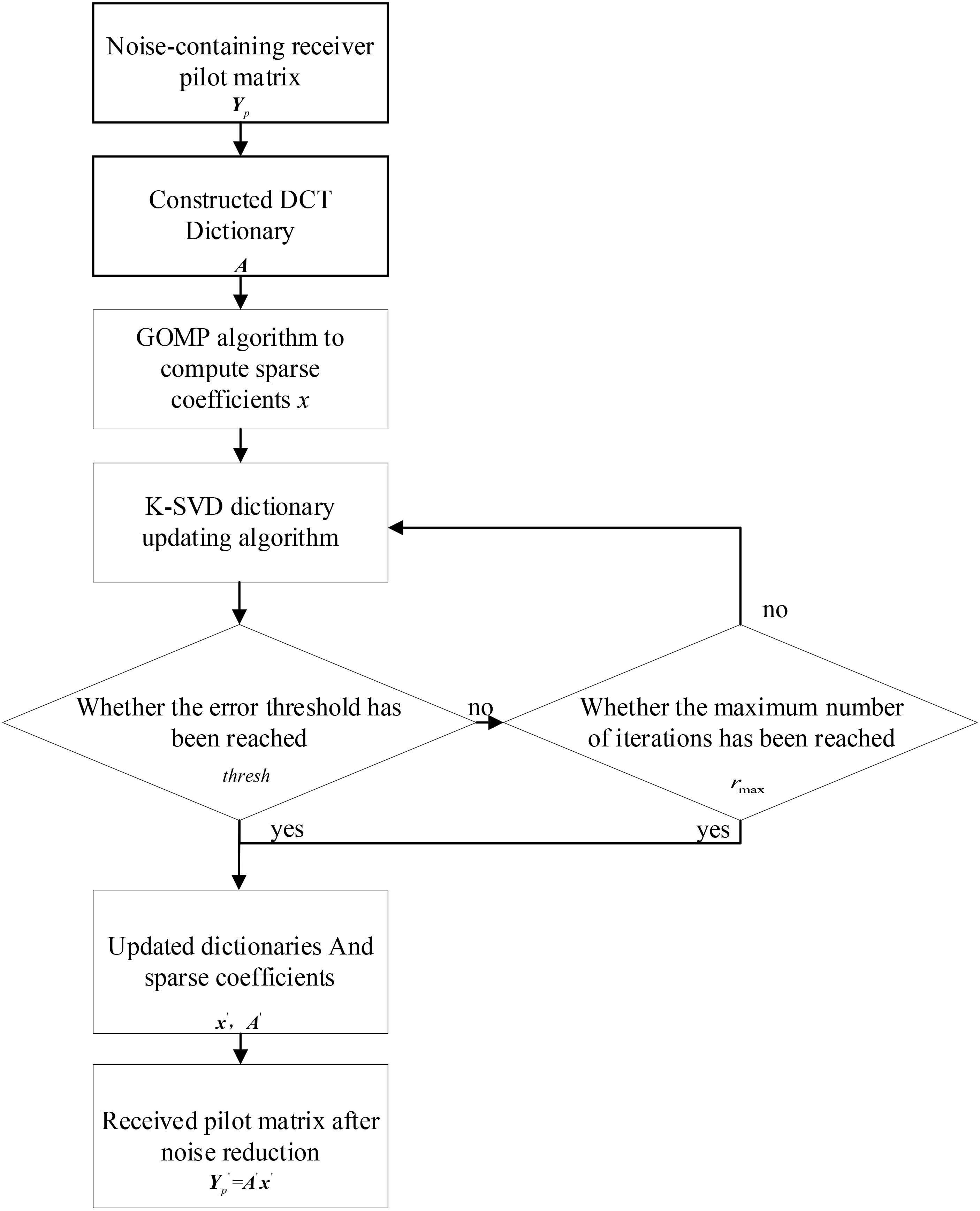
Figure 2. Flowchart of KSVD dictionary learning algorithm for noise reduction.

3.2 A priori knowledge acquisition based on GOMP channel estimation

Obtaining the time-domain shock response of the underwater acoustic channel using GOMP channel estimation algorithm h_GOMP. To obtain the a priori knowledge of the TMSBL, the initial parameters of the EM algorithm are chosen based on the characteristics of the underwater acoustic channel, effectively reducing the algorithm’s complexity.

Time-domain impact response of underwater acoustic channel obtained using GOMP channel estimation algorithm.

$\begin{array}{ll}\begin{array}{c}{\mathit{h}}_{\text{GOMP}}={}_h^{\text{argmin}}{\Vert {\mathit{Y}}_p}^{\prime }-{\mathit{\Phi }}_{p,{\Lambda }_i}{\mathit{h}}_i\Vert \end{array}& (20)\end{array}$

where ${\Phi }_{p,{\Lambda }_i}$ is the perceptual matrix corresponding to the set of indexes after the ith update of atoms, and h_i is the channel estimate after the ith iteration.

Set the average energy superposition function Q of the channel to be (Hong et al., 2022):

$\begin{array}{ll}\begin{array}{c}Q=\frac{1}{L}{\displaystyle \sum _{i=1}^L}{\mathit{h}}_{\text{GOMP}}i\end{array}& (21)\end{array}$

Among them. h_GOMPi is the ith column of ${\mathit{h}}_{\text{GOMP}}$, i.e., the channel time-domain impulse response of the ith OFDM symbol.

Set the threshold as $T_Q=\alpha \text{max}(Q)$ where α is the energy coefficient, determined based on the characteristics of the underwater acoustic channel and considering the computational complexity. Compare the channel average energy superposition function Q and the threshold T_Q of the channel:

$\begin{array}{ll}\begin{array}{c}{\mathit{\Omega }}_{\text{GOMP}}(i)=\{\begin{array}{c}1, Q(i)\ge T_Q\\ 0, Q(i)<T_Q\end{array} i=1,2,\dots ,M.\end{array}& (22)\end{array}$

where ${\mathit{\Omega }}_{\text{GOMP}}$ is the hyperparameter vector of TMSBL. When the channel average energy superposition function Q is greater than the threshold, indicating that, at this time, the hyperparameter control channel impulse response is the channel tapping coefficient, ${\mathit{\Omega }}_{\text{GOMP}}=1$; on the contrary, it is considered that the hyperparameter is too small and its control channel impulse response probability is the noise, the ${\mathit{\Omega }}_{\text{GOMP}}=0$.

Define the initial hyperparameter matrix as $\mathit{\Gamma }=\text{diag}({\mathit{\Omega }}_{\text{GOMP}})$, whose diagonal elements are hyperparameter vectors ${\mathit{\Omega }}_{\text{GOMP}}$. Take the positions Γ whose diagonal elements are equal to zero as the indexed set s and eliminate the atoms corresponding to $s$ in the dictionary matrix ${\mathit{\Phi }}_p$ to obtain the initialized dictionary matrix ${\mathit{\Phi }}_p^{\text{'}}$ of the improved TMSBL algorithm.

Finally, the noise-canceled pilot receiver matrix ${\mathit{Y}}_p^{\text{'}}$, the initial hyperparameter matrix Γ, and the initialized dictionary matrix ${\Phi }_p^{\text{'}}$ are substituted into the TMSBL channel estimation method for underwater acoustic channel estimation.

4 Simulation results and analysis

The simulation to validate the performance of the proposed algorithm is conducted using the implementation of an underwater acoustic OFDM communication system. An OFDM symbol comprises 1024 subcarriers, with 256 designated as frequency-conducting subcarriers (utilizing a comb-conducting structure), 30 as null subcarriers, and 738 as data subcarriers. Sixty-five OFDM symbols are transmitted in each frame, and the signal is modulated using 16QAM. The specific OFDM parameters are configured as presented in Table 1.

Table 1

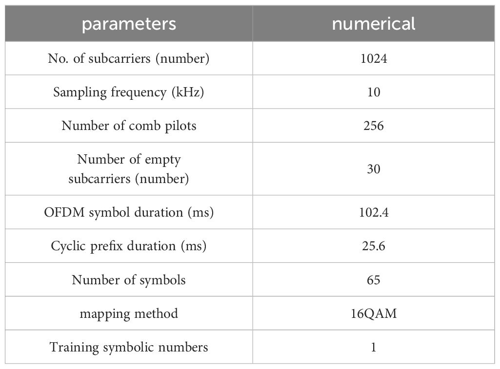
Table 1. OFDM system parameter settings.

The simulated channel is generated using the BELLHOP underwater acoustic channel model to obtain the underwater acoustic channel impulse response. The sound velocity profile of the real marine environment, as experimented in the Yellow Sea in 2013, is depicted in Figure 3. This sound velocity profile is imported into BELLHOP, setting the sound source depth to 10m, the hydrophone depth to 9m, and the distance between the two to be 2000m. The seafloor is modeled as an elastic seafloor with seawater density of 1.5g/cm³, seafloor absorption of 0.5dB, and the resulting channel impulse response is shown in Figure 4 as obtained through simulation. The seabed absorption is 0.5dB, and the sound line grazing angle is [-35°, 35°], leading to the channel impulse response displayed in Figure 4, obtained through simulation.

Figure 3

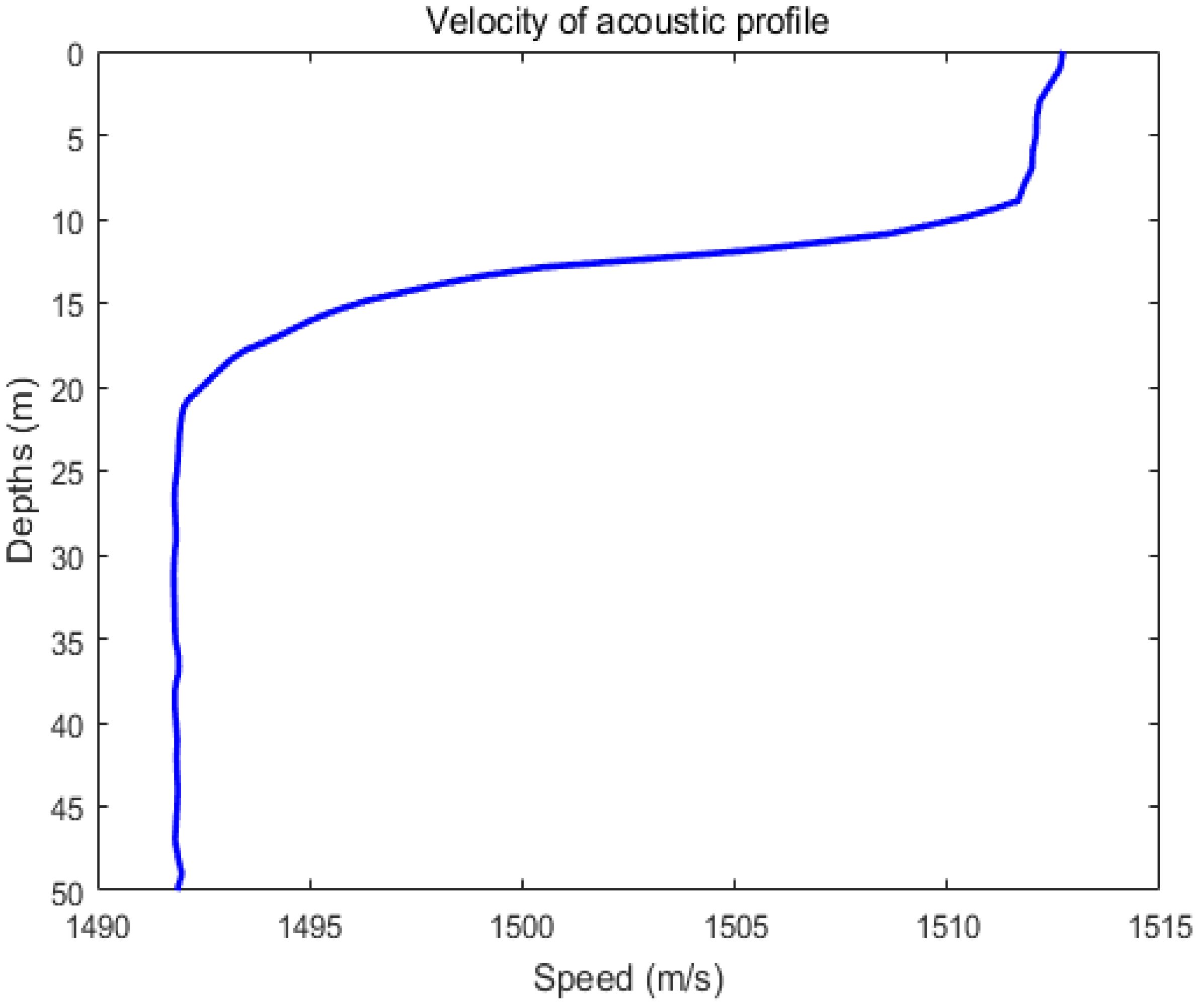
Figure 3. Velocity of acoustic profile.

Figure 4

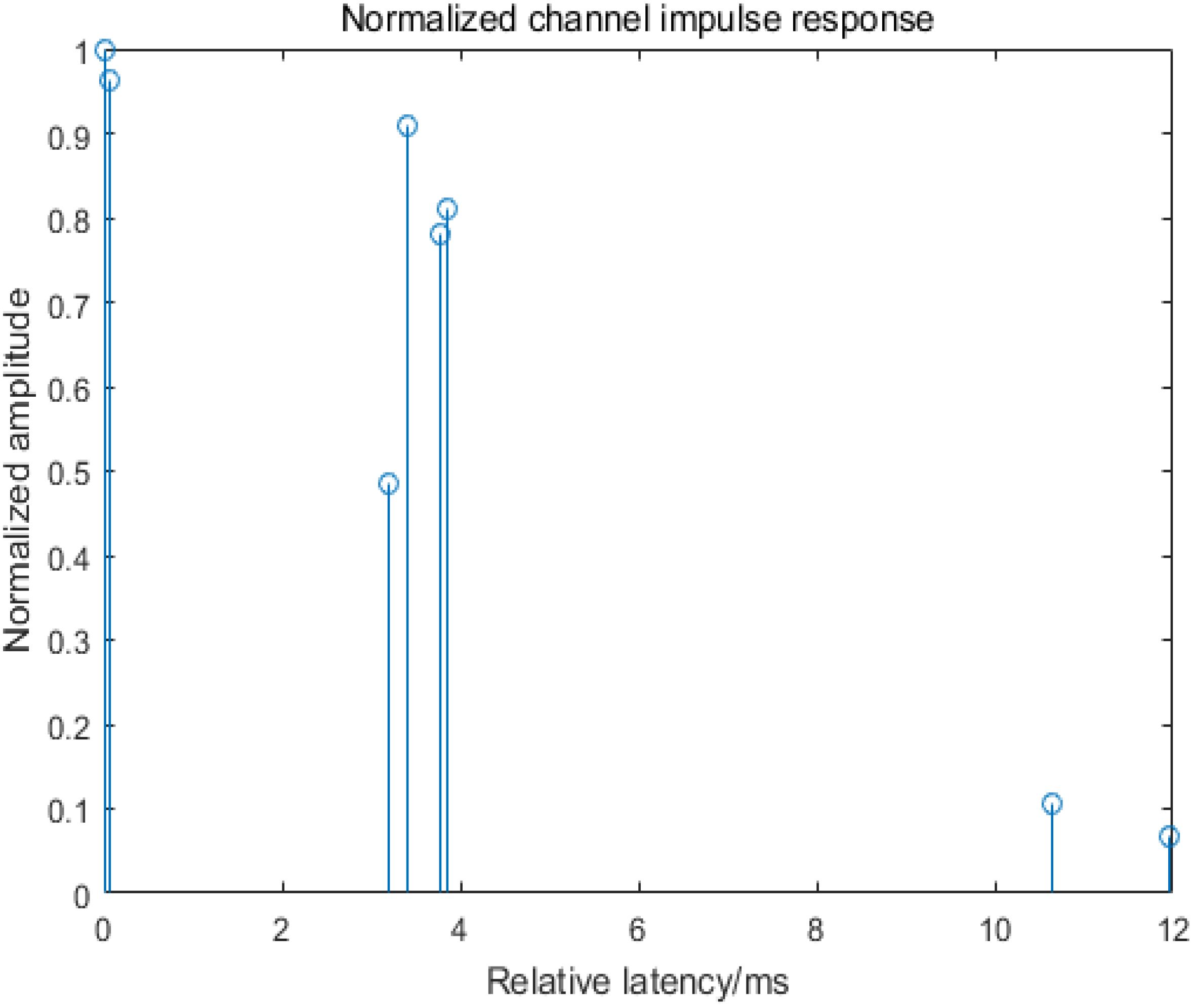
Figure 4. Channel impulse response.

In order to measure the estimation accuracy of the proposed algorithm, the normalised mean square error (NMSE) of the channel estimation is defined as:

$\begin{array}{ll}\begin{array}{c}NMSE=({\displaystyle \sum _{i=0}^{L-1}}\Vert \widehat{{\mathit{h}}_i}-\mathit{h}{\Vert }_F^2/\Vert \mathit{h}{\Vert }_F^2)/L\end{array}& (23)\end{array}$

where $\widehat{{\mathit{h}}_i}$ denotes the channel estimate of the ith OFDM symbol, h is the true OFDM underwater acoustic channel impulse response, and L is the number of OFDM symbols.

The primary simulated comparison algorithms include LS, GOMP, TMSBL, and the enhanced TMSBL with the LS priori knowledge acquisition (LS-TMSBL) (Hong et al., 2022). The simulation is divided into two main aspects: firstly, the comparison of the normalized mean square error of the channel estimation to verify the performance of the channel estimation method; secondly, the comparison of the time used for the channel estimation to verify the complexity of the channel estimation method.

4.1 Simulation results and performance analysis

The proposed algorithm is described as KSVD-GOMP-TMSBL algorithm for simplicity of expression. The main comparison algorithms for the simulation are LS, GOMP, TMSBL, and LS-TMSBL methods, setting the maximum number of iterations $r_{\text{max}}=5000$ and the error threshold is $\text{thresh}=1\times {10}^{-6}$.

Figure 5 displays the normalized mean square error plots for channel estimation using LS, GOMP, TMSBL, LS-TMSBL, and KSVD-GOMP-TMSBL algorithms. The received pilot matrix was denoised using the K-SVD dictionary learning method. The energy coefficient α is set to 0.05, and GOMP sparsity is fixed at 30. It can be observed from Figure 5 that the LS algorithm, devoid of channel sparsity utilization, exhibits poor estimation performance. The GOMP algorithm slightly outperforms the LS algorithm. The TMSBL algorithm, capitalizing on both the sparse nature of the channel and the temporal correlation between different symbols, demonstrates superior performance in channel estimation. The LS-TMSBL algorithm, incorporating the LS algorithm to acquire a priori knowledge of the TMSBL algorithm and influenced by the energy coefficient, exhibits performance slightly lower than the TMSBL algorithm. The KSVD-GOMP-TMSBL algorithm, leveraging the K-SVD dictionary learning algorithm for noise reduction, GOMP to obtain a priori knowledge of the TMSBL, and null subcarriers to determine noise variance, demonstrates improved performance compared to the comparison algorithms.

Figure 5

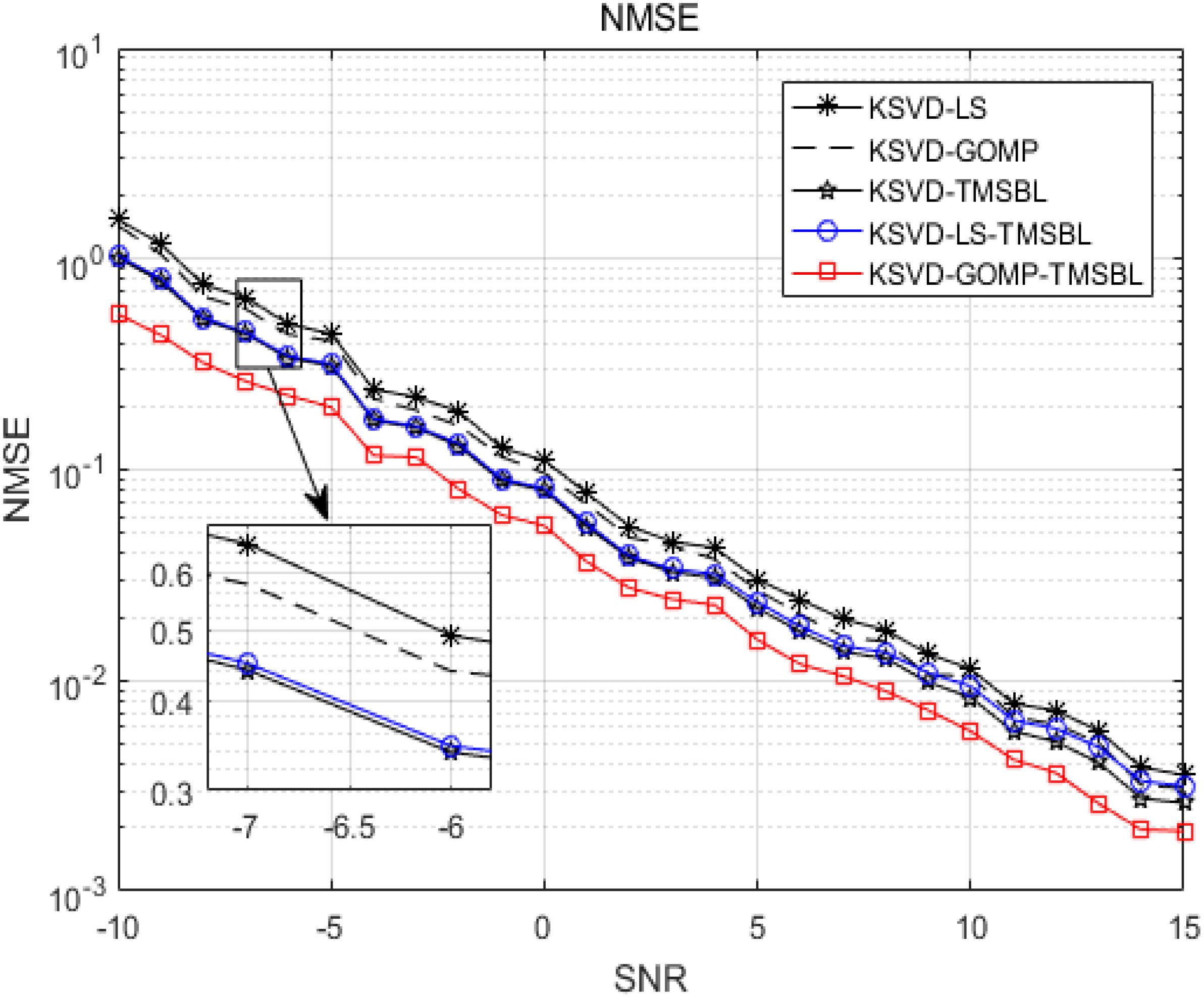
Figure 5. Channel estimation error with K-SVD dictionary learning noise reduction.

Figure 6 displays the normalized mean square error plots for channel estimation using LS, GOMP, TMSBL, LS-TMSBL, and KSVD-GOMP-TMSBL algorithms. No denoising was applied to the received pilot matrix. The energy coefficient α is set to 0.05, and GOMP sparsity is fixed at 30. It is evident from Figure 6 that, without noise reduction, the LS algorithm is more susceptible to noise, leading to a degradation in the performance of the LS-TMSBL algorithm. In contrast, the TMSBL algorithm and the KSVD-GOMP-TMSBL algorithm are relatively less affected by noise. The KSVD-GOMP-TMSBL algorithm improve its performance by obtaining the null subcarrier through noise variance.

Figure 6

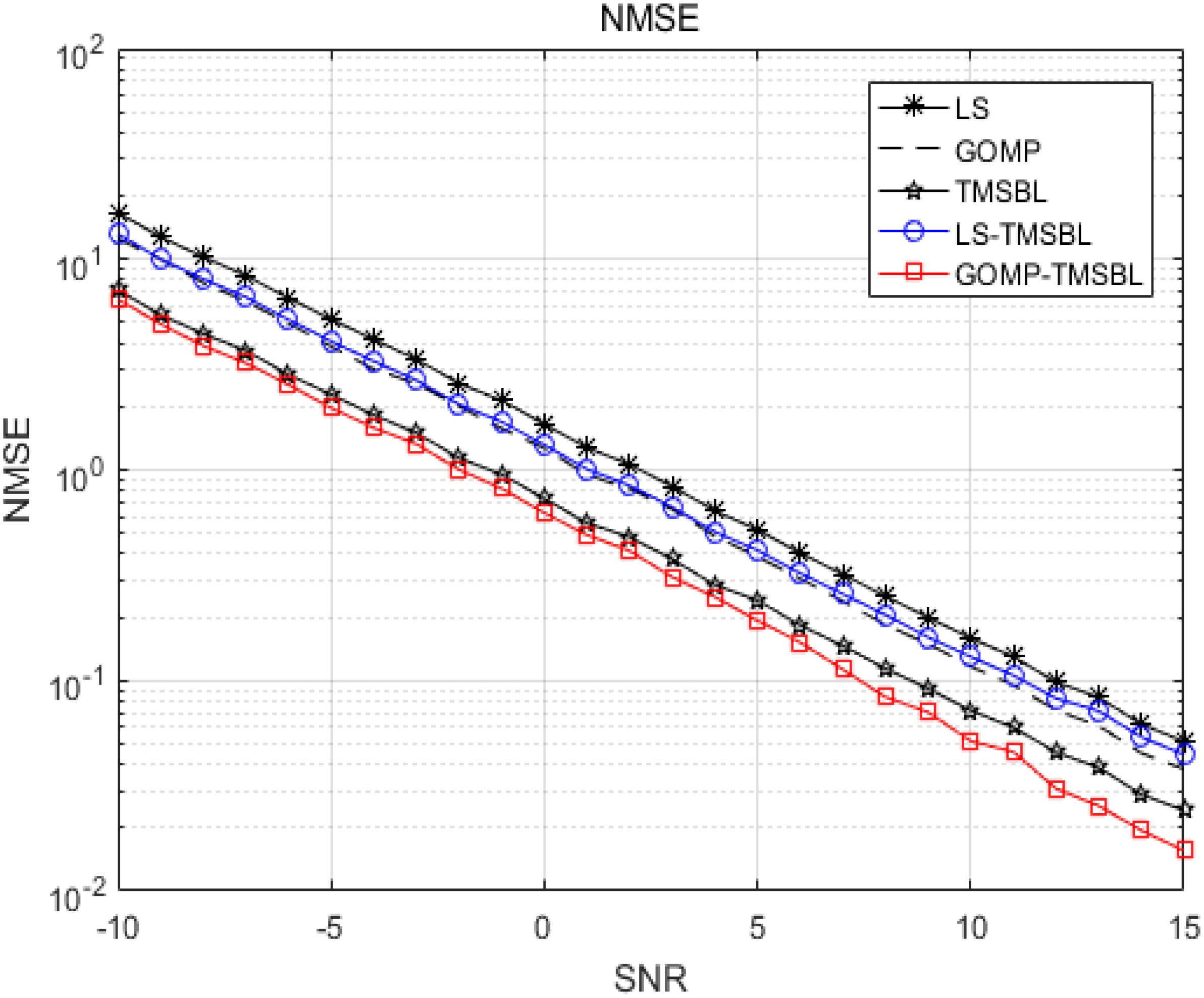
Figure 6. Channel estimation error without noise reduction processing.

Overall, the KSVD-GOMP-TMSBL algorithm exhibits improved channel estimation performance. The use of the K-SVD dictionary learning algorithm for noise reduction on the received pilot matrix enables the algorithm to achieve accurate estimation results even at low SNR. The algorithm’s performance is further enhanced by obtaining precise noise variance through null subcarriers instead of iteratively updating the noise variance. Additionally, the algorithm demonstrates some improvement in estimation performance even without noise reduction processing, showcasing its ability to mitigate certain noise interferences. The factors influencing the KSVD-GOMP-TMSBL algorithm are subsequently analyzed from various perspectives.

First, discuss the impact of the dictionary learning noise reduction method on the algorithm’s performance. Figure 7 shows the lofar plot (left) of the received pilot matrix at an SNR of -10dB and the lofar plot (right) of the received pilot matrix after noise reduction using dictionary learning. It is clear that the lofar plots are significantly clearer after noise reduction. The SNR of the received pilot matrix before noise reduction is -10.28dB, and after noise reduction, it improves to 2.36dB. This demonstrates the superior noise reduction effect of the dictionary learning algorithm on the received matrix.

Figure 7

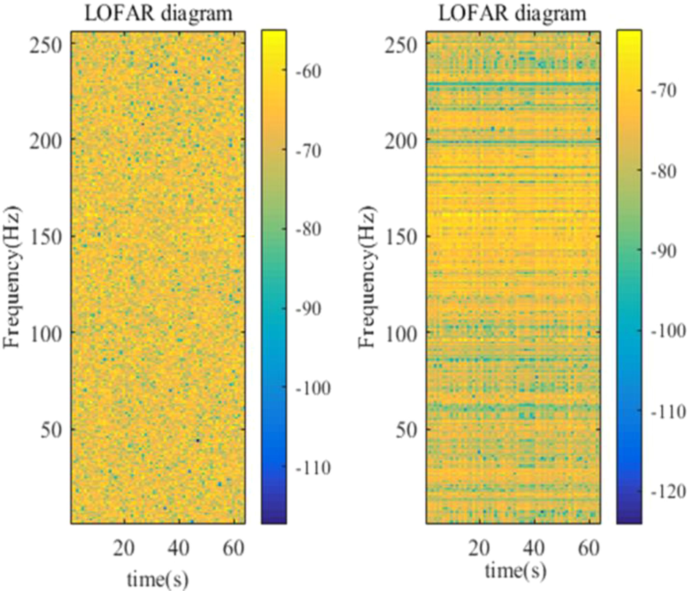
Figure 7. Lofar comparison figure of receive pilot matrix before(left) and after(right) noise reduction.

In Figure 8, compare the effectiveness of noise reduction between the dictionary learning algorithm and the singular value decomposition (SVD) noise reduction method. The figure demonstrates the impact of two noise reduction methods on the performance of both the TMSBL and GOMP-TMSBL algorithms. From Figure 8, the dictionary learning noise reduction method significantly improves channel estimation in both algorithms compared to the singular value decomposition method. For the GOMP-TMSBL algorithm, the NMSE of channel estimation under the dictionary learning noise reduction method is 0.0566, representing an almost tenfold decrease compared to the singular value decomposition noise reduction method. This demonstrates that the dictionary learning noise reduction method is highly effective in noise reduction.

Figure 8

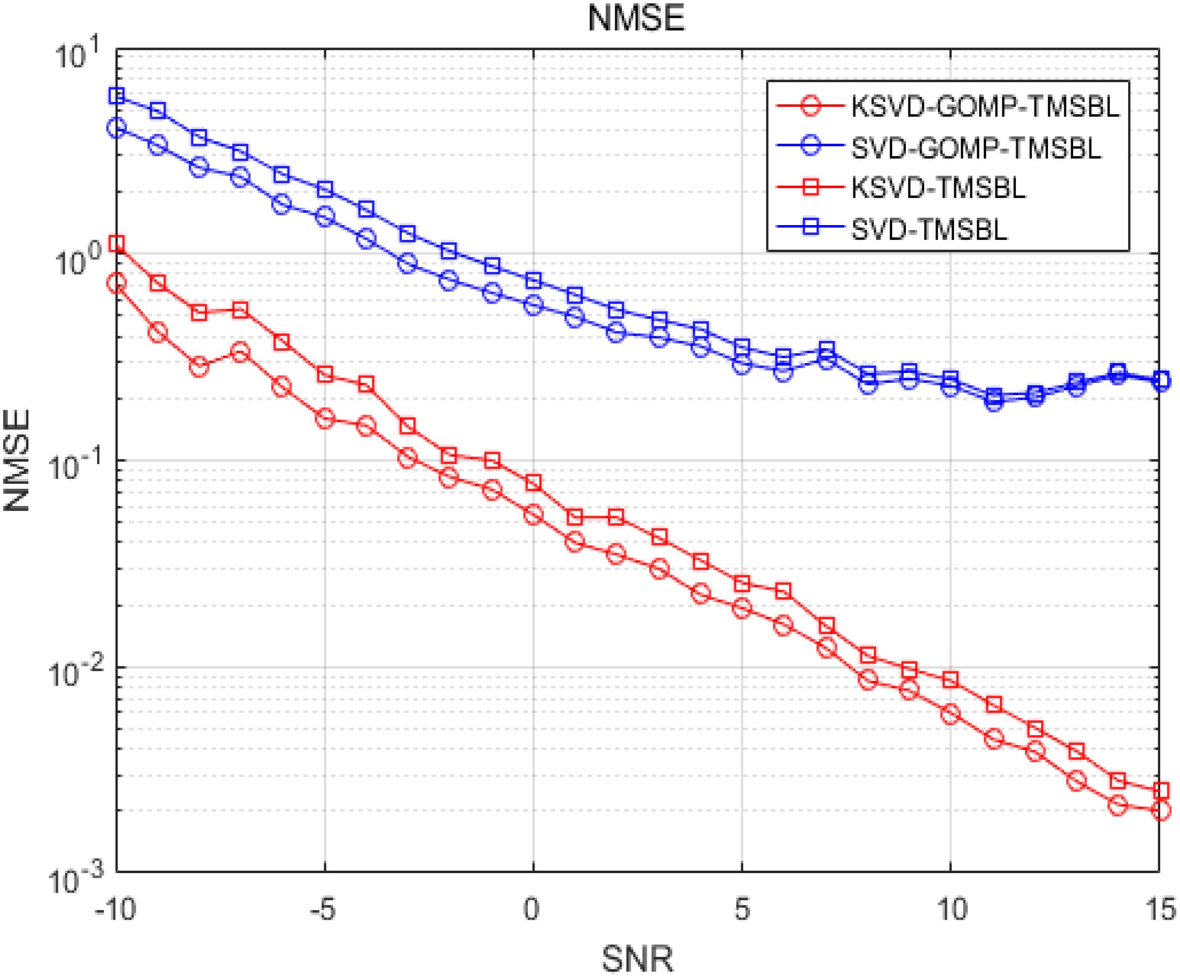
Figure 8. Channel estimation error with different noise reduction methods.

Figure 9 compares the channel estimation error of the KSVD-GOMP-TMSBL algorithm with other comparison algorithms, without noise reduction processing, to investigate the impact of dictionary learning noise reduction algorithms on the performance of channel estimation methods. As shown in Figure 9, the estimation error of the GOMP-TMSBL algorithm is 6.616, while the estimation error of the KSVD-GOMP-TMSBL algorithm is 0.5973 at a signal-to-noise ratio of -10 dB. The estimation error of the KSVD-GOMP-TMSBL algorithm is reduced by approximately 91.1% compared to the GOMP-TMSBL algorithm. This indicates that the performance of the channel estimation algorithm is improved by performing noise reduction on the received pilot matrix using the dictionary learning algorithm.

Figure 9

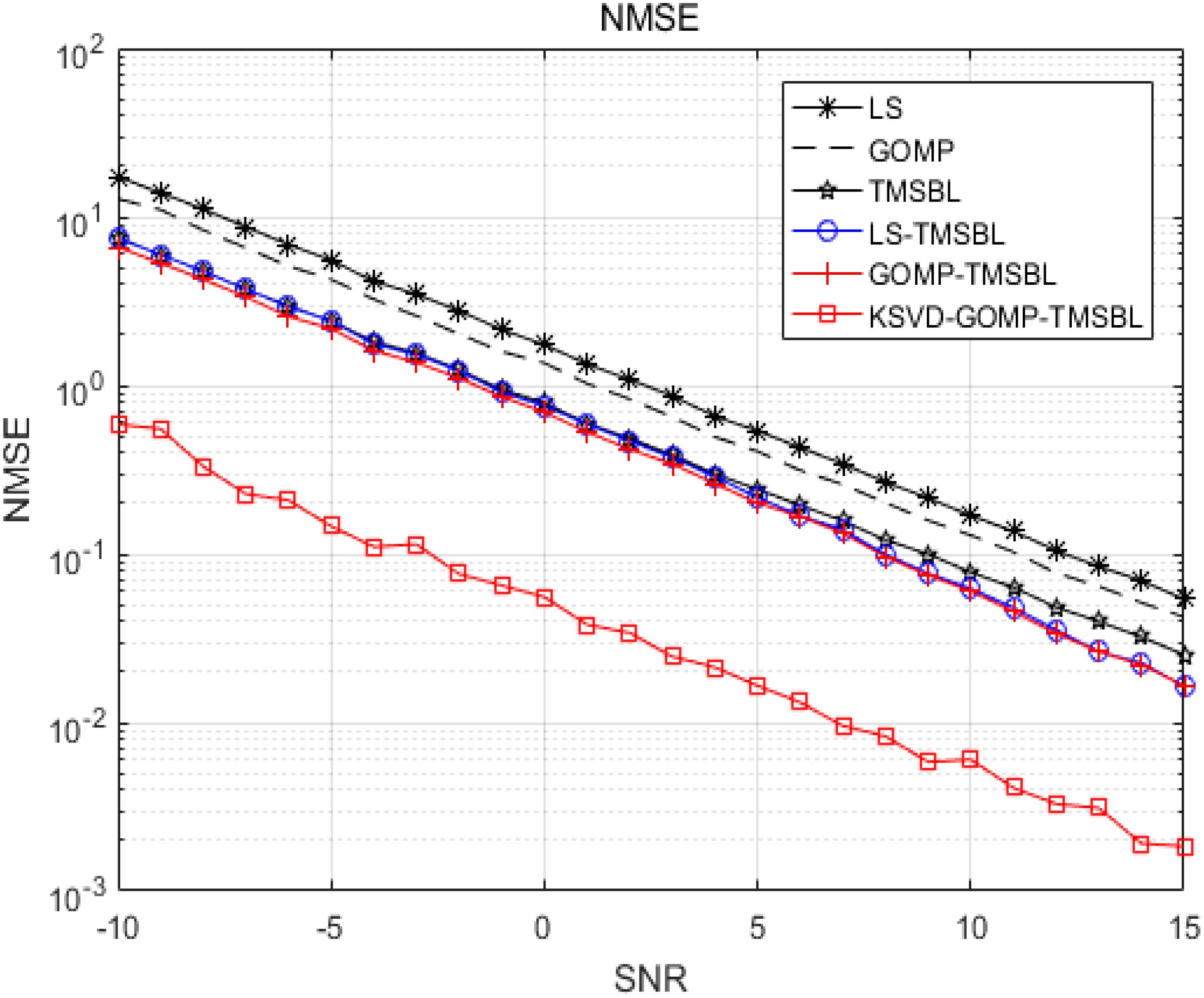
Figure 9. Channel estimation error with and without noise reduction.

Next, discuss the impact of the energy coefficient (α) on the KSVD-GOMP-TMSBL algorithm. The KSVD-GOMP-TMSBL algorithm in the α value will affect the size of the threshold and, consequently, the hyperparameter matrix. When the α value is too small, the threshold becomes insufficient, leading to noise being misestimated as channel tapping coefficients, thereby affecting the accuracy of channel estimation. Conversely, when the α value is too large, the threshold becomes excessive, causing real but smaller channel tapping coefficients to be mistaken as noise, thus affecting the algorithm’s performance. The chosen value of α significantly impacts the performance of the KSVD-GOMP-TMSBL algorithm. Figure 10 shows the energy coefficient α channel estimation error when different values are taken, where the GOMP algorithm sparsity is taken to be 30. From the figure, it can be observed that when the $0.01\le \alpha \le 0.10$ the estimation errors of the KSVD-GOMP-TMSBL algorithms are relatively close, both achieve a better performance. When $\alpha =0.15$, the estimation performance of the KSVD-GOMP-TMSBL algorithm is closer to that when α takes the value in the range [$0.01~0.10$]. However, as the threshold is critical at a = 0.15, confusion between channel tapping coefficients and noise can arise, which affects the algorithm’s stability, exhibiting significant fluctuations when the signal-to-noise ratio is 11dB. For $\alpha >0.15$, the estimation performance of the KSVD-GOMP-TMSBL algorithm is poorer, and it is slightly inferior to the TMSBL algorithm when the signal-to-noise ratio reaches a certain value. Therefore, to ensure optimal channel estimation performance and algorithm stability, the value of α should be in the range of [$0.01~0.10$].

Figure 10

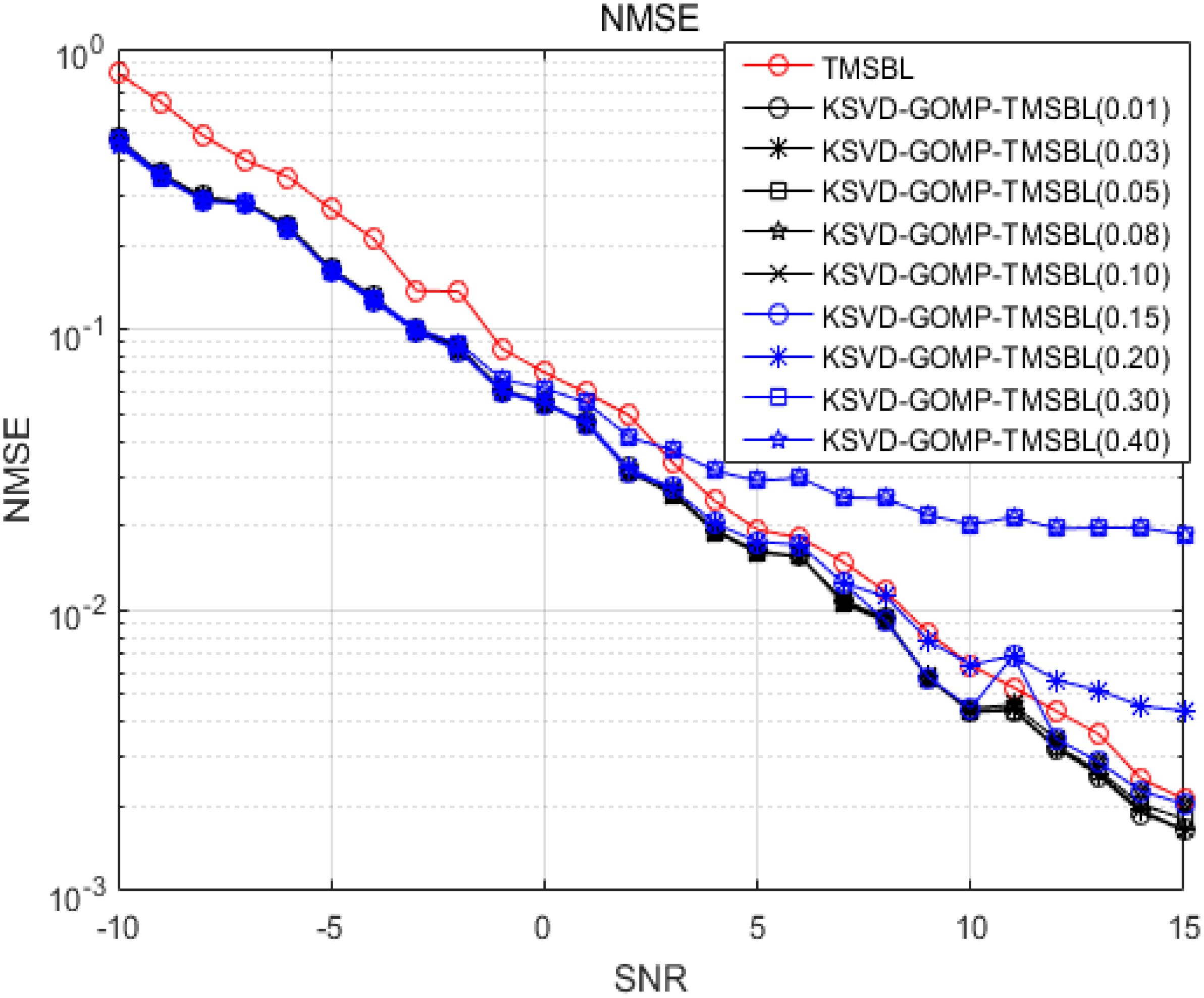
Figure 10. Channel estimation error for different energy coefficients.

The performance of the conventional GOMP algorithm is notably influenced by sparsity. Figure 11 illustrates the channel estimation error of the GOMP algorithm with varying sparsity values, with the energy coefficient (α) set to 0.05. It is evident from the figure that the subpar channel estimation performance when the sparsity is 5 is attributed to the multipath complexity of the shallow sea environment. In such an environment, where the number of propagated multipaths is higher, opting for a small sparsity value may erroneously set the channel’s tapping coefficient to 0 when deriving hyperparameters from the a priori knowledge of the TMSBL. This leads to a biased channel estimation. The performance of the KSVD-GOMP-TMSBL algorithm is more consistent when the sparsity is set to the other five values, all of which surpass the TMSBL algorithm, enabling superior estimation performance. Thus, the KSVD-GOMP-TMSBL algorithm only needs to adopt a larger sparsity value, as the algorithm is minimally affected by the specific value of sparsity. Consequently, the performance of the KSVD-GOMP-TMSBL algorithm is not influenced by the sparsity chosen by the GOMP algorithm.

Figure 11

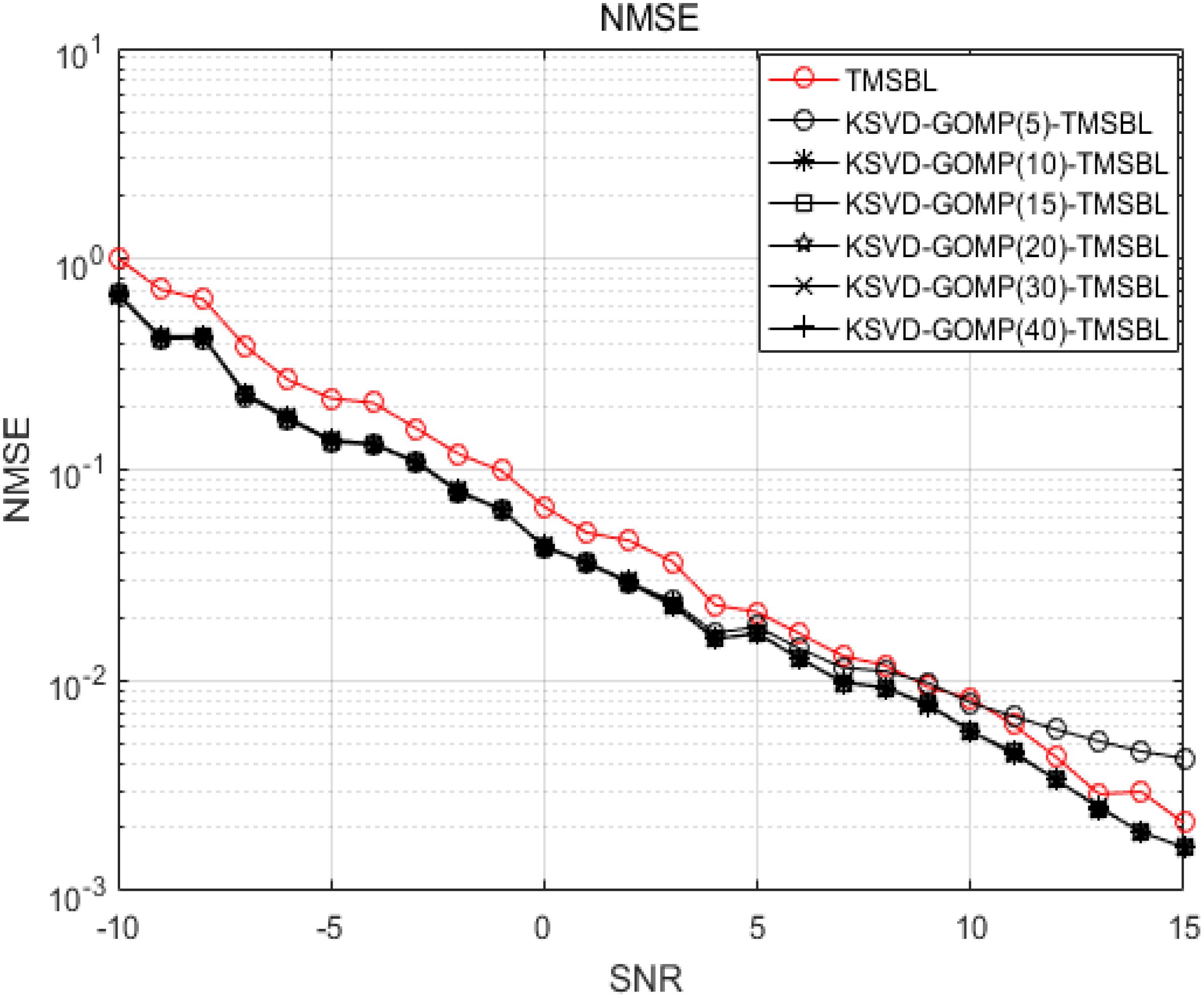
Figure 11. NMSE for different sparsities.

The influence of noise variance calculation methods on the performance of the TMSBL algorithm and the KSVD-GOMP-TMSBL algorithm is discussed below. Figure 12 illustrates the channel estimation errors of the KSVD-GOMP-TMSBL algorithm employing two noise variance calculation methods. At an SNR of -10 dB, the NMSE of the channel estimation for the KSVD-GOMP-TMSBL algorithm is 1.058 when the noise variance is computed through iterative updating using (Equation 13). Conversely, the NMSE is reduced to 0.5579 when the noise variance is determined using the null subcarrier in conjunction with (Equation 14). Compared to the previous method, employing null subcarriers to acquire the noise variance diminishes the NMSE of the channel estimation of the KSVD-GOMP-TMSBL algorithm by approximately 47.27%. It is evident that utilizing the null subcarrier to determine noise variance in the OFDM system can enhance the performance of the KSVD-GOMP-TMSBL algorithm and improve the accuracy of channel estimation.

Figure 12

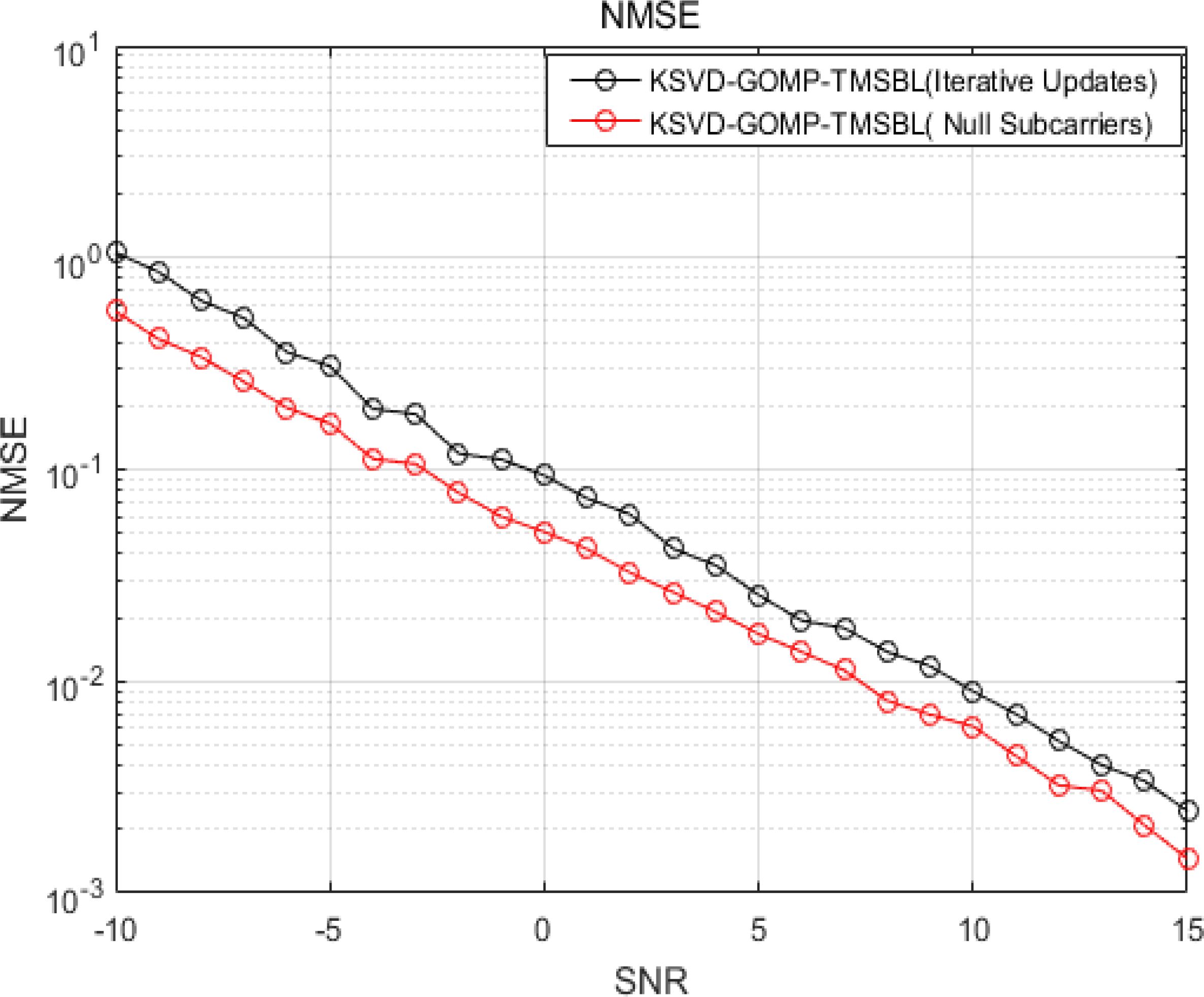
Figure 12. Channel estimation errors calculated with different noise variances.

In the following sections, the proposed algorithm is compared with other methods. Figure 13 illustrates the NMSE of various channel estimation methods. The SBL method (Wipf and Rao, 2004) addresses the multi-measurement model by sequentially processing columns to estimate the channel. The TMSBL method (Qiao et al., 2018) leverages temporal correlation between channels to address the multi-measurement model. The SVD-LS-TMSBL method (Hong et al., 2022) utilizes SVD to reduce noise, LS to acquire a priori knowledge for the TMSBL algorithm, and TMSBL to achieve joint channel estimation. The figure illustrates that the SBL method exhibits the highest NMSE, which can be attributed to its failure to leverage the correlation between the channels. In contrast, TMSBL demonstrates superior channel estimation accuracy compared to the SBL algorithm due to its ability to capitalize on the temporal correlation between the underwater acoustic channels. The SVD-LS-TMSBL algorithm achieves lower NMSE in channel estimation than the TMSBL algorithm because it integrates singular value decomposition for noise reduction and employs the LS method to acquire the priori knowledge for the TMSBL algorithm. The KSVD-GOMP-TMSBL algorithm employs K-SVD dictionary learning for noise reduction, with a priori knowledge for the TMSBL algorithm obtained through the GOMP algorithm. This approach effectively addresses the limitations of the SVD-LS-TMSBL algorithm, where the LS channel estimation method is more sensitive to noise, and the noise reduction capability of SVD is suboptimal in low SNR environments, leading to reduced channel estimation accuracy. These results demonstrate that the KSVD-GOMP-TMSBL method achieves superior channel estimation performance compared to the other algorithms. It can be observed that the proposed algorithm is capable of effectively reducing the impact of noise on the TMSBL algorithm, thereby enhancing the accuracy of channel estimation in OFDM communication systems.

Figure 13

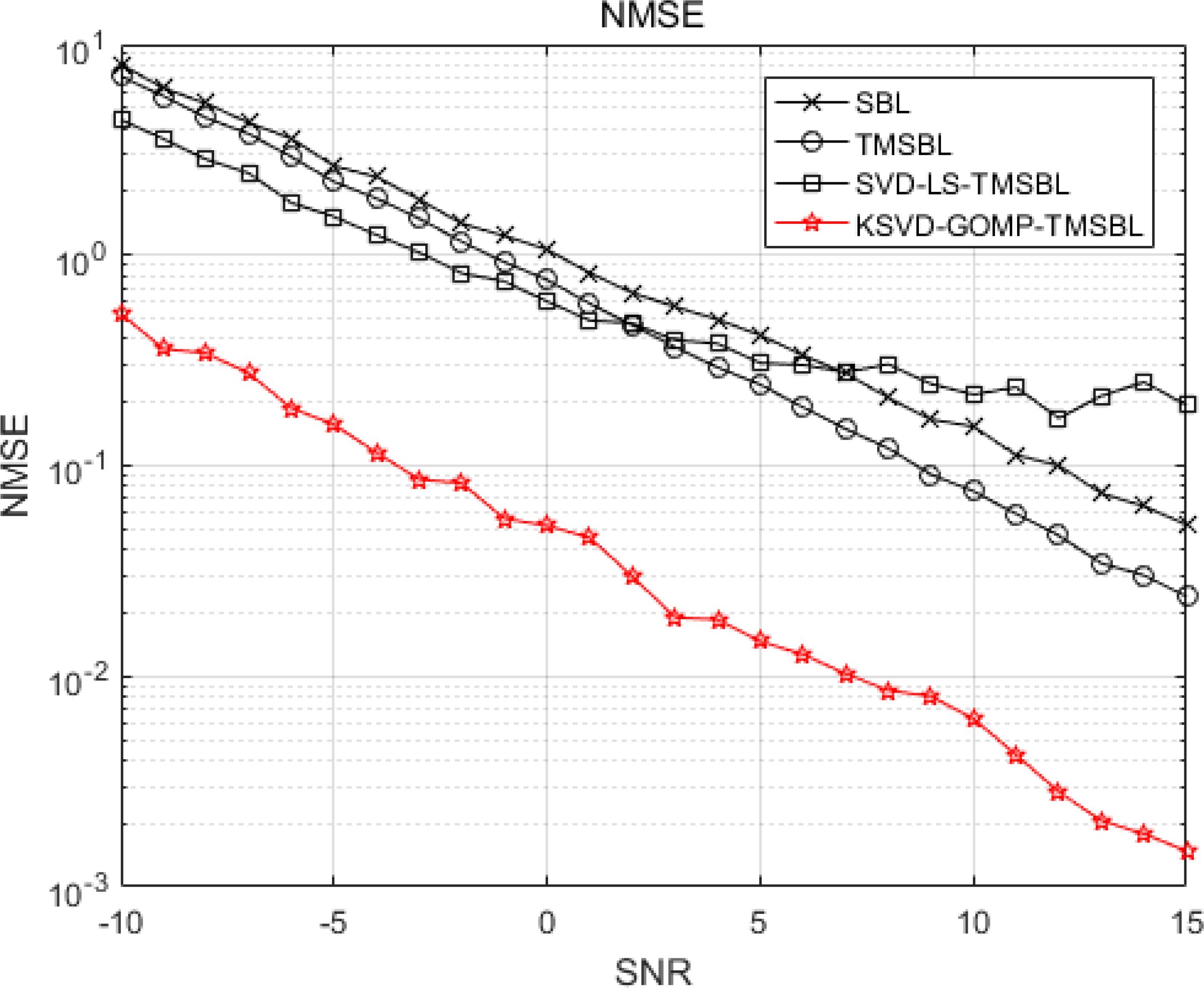
Figure 13. NMSE for different channel estimation methods.

The subsequent analysis centers on the influence of the KSVD-GOMP-TMSBL algorithm on the performance of the OFDM communication system. Figure 14 illustrates the bit error rate (BER) of various channel estimation methods, suggesting that the performance of the OFDM communication system is improved by the KSVD-GOMP-TMSBL algorithm. With an increase in SNR, all five channel estimation methods represented in the figure demonstrate a reduction in the BER of the OFDM communication system. At an SNR of 15 dB, the BERs for the LS, GOMP, TMSBL, LS-TMSBL, and KSVD-GOMP-TMSBL algorithms are 6.2%, 5.7%, 5.8%, 5.3%, and 4.5%, respectively. In comparison to the benchmark algorithms, the BER of the KSVD-GOMP-TMSBL algorithm decreases by at least approximately 15.1%. Based on the aforementioned analysis, the KSVD-GOMP-TMSBL algorithm contributes to the enhancement of the OFDM communication system’s performance.

Figure 14

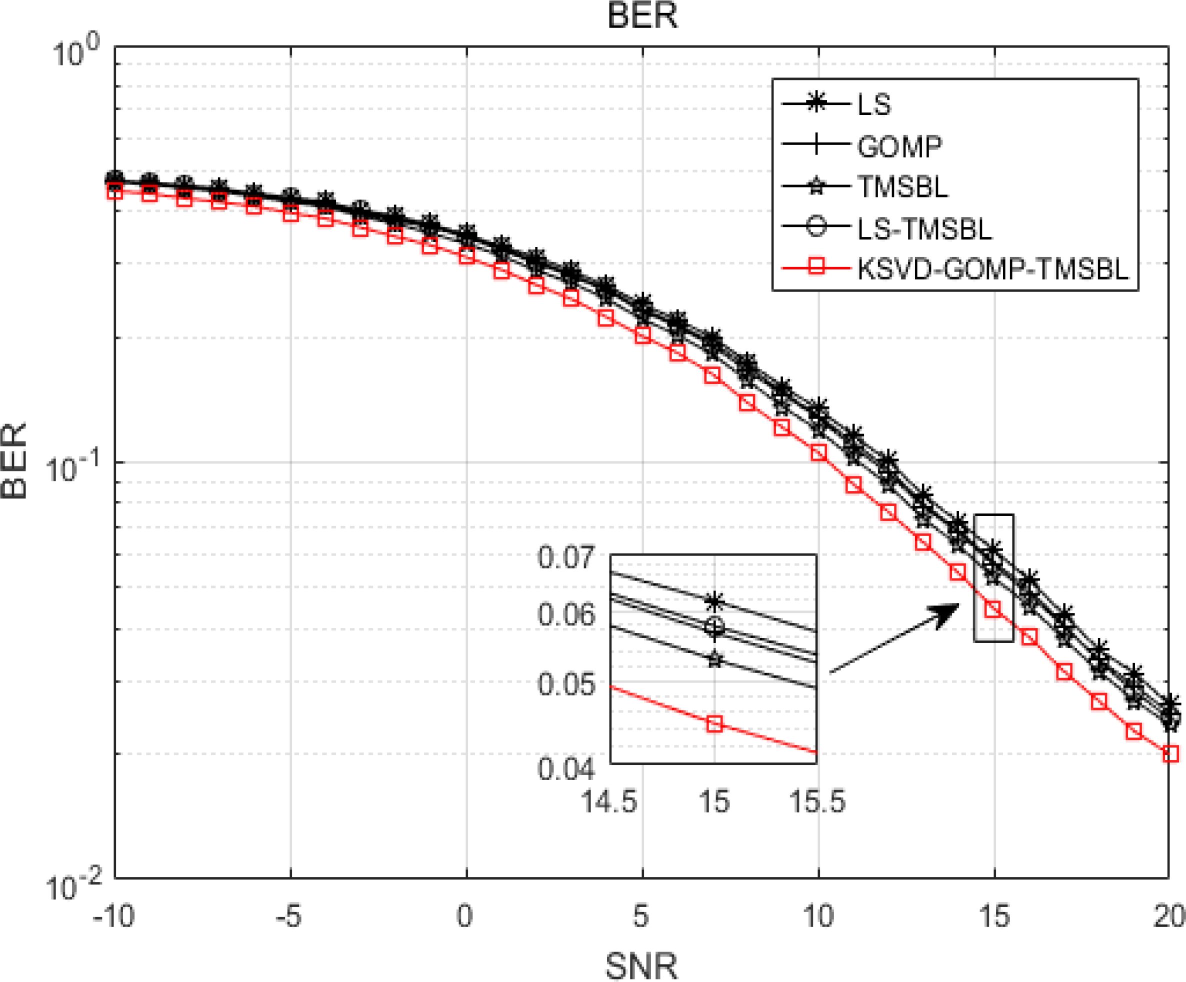
Figure 14. BER for different channel estimation methods.

Table 2 presents the estimation errors of various channel estimation methods under identical signal-to-noise ratio conditions. The results clearly indicate that the estimation accuracy of the KSVD-GOMP-TMSBL algorithm is markedly improved compared to other methods. At a signal-to-noise ratio of -10 dB, the channel estimation error of the KSVD-GOMP-TMSBL algorithm decreases by around 96.6%, 95.4%, 92.2%, and 92.1% compared to the LS, GOMP, TMSBL, and LS-TMSBL channel estimation methods, respectively. The estimation error of the KSVD-GOMP-TMSBL algorithm similarly decreases across other signal-to-noise ratio values. This confirms the significant enhancement in channel estimation accuracy achieved by the KSVD-GOMP-TMSBL algorithm.

Table 2

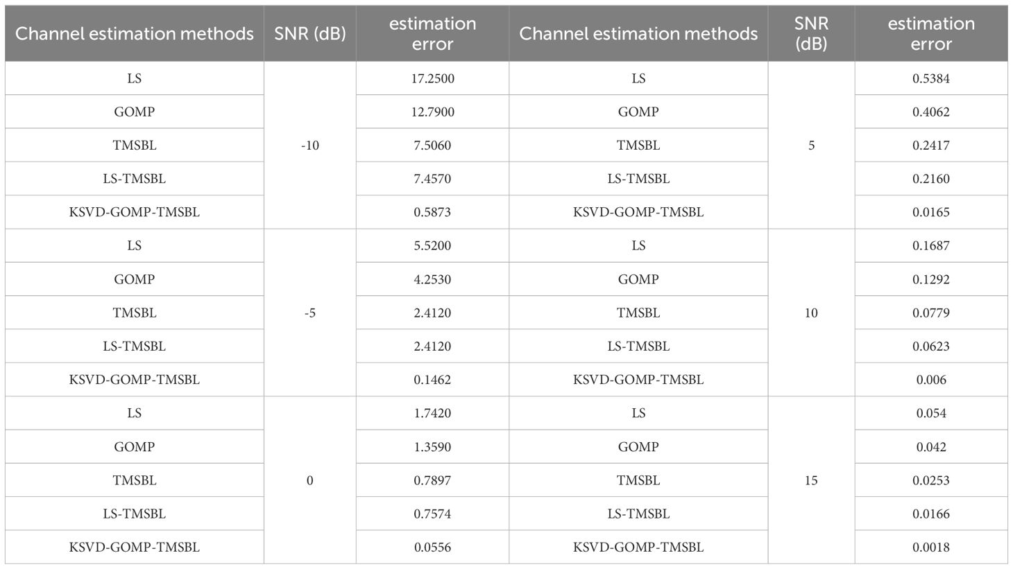
Table 2. Estimation errors of different channel estimation methods.

4.2 Algorithm complexity analysis

The following section will analyze the convergence and convergence rate of the KSVD-GOMP-TMSBL algorithm. Figure 15 illustrates the NMSE of the TMSBL and KSVD-GOMP-TMSBL algorithms for varying numbers of iterations at a signal-to-noise ratio (SNR) of -10 dB. It can be observed that both algorithms demonstrate convergence as the number of iterations increases. The KSVD-GOMP-TMSBL algorithm reaches convergence at 7 iterations, while the TMSBL algorithm reaches convergence at 26 iterations. The results demonstrate that the KSVD-GOMP-TMSBL algorithm exhibits a faster convergence rate than the TMSBL algorithm. It has been demonstrated that the integration of the KSVD-GOMP-TMSBL algorithm for noise reduction based on a KSVD dictionary and the utilization of GOMP to derive the prior knowledge of the TMSBL algorithm can effectively reduce the number of iterations of the TMSBL algorithm and accelerate the convergence speed.

Figure 15

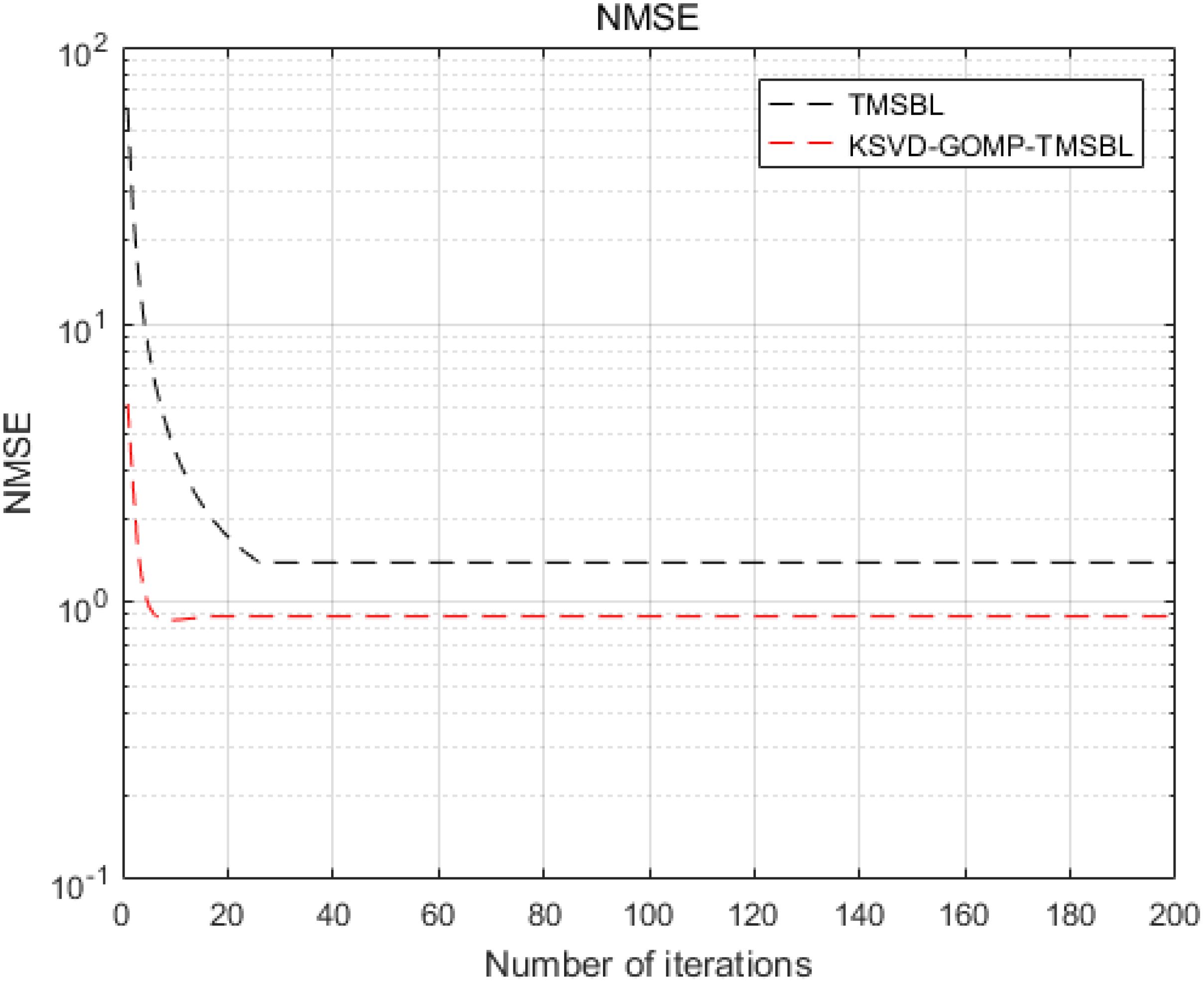
Figure 15. NMSE of TMSBL algorithm and KSVD-GOMP-TMSBL algorithm at different numbers of iterations.

The KSVD-GOMP-TMSBL algorithm is primarily composed of three key components: KSVD dictionary learning for noise reduction, a priori knowledge acquisition based on GOMP channel estimation, and TMSBL algorithm channel estimation. The KSVD dictionary learning technique for noise reduction incorporates GOMP sparse coding and dictionary updating. The computational complexity of GOMP sparse coding is $O(kpJL)$, and that of dictionary updating is $O(pJL(L+1))$. Consequently, the computational complexity of KSVD dictionary learning noise reduction is $O(pJL(k+L+1))$. The computational complexity of acquiring a priori knowledge through GOMP channel estimation is $O(kpJL+ML)$. The computational complexity of TMSBL channel estimation is $O(N(M^{2}p+L^4+L^{2}M))$, where N represents the number of iterations. In conclusion, the principal computational complexity of the KSVD-GOMP-TMSBL algorithm is $O(pJL(k+L+1)+ML+N(M^{2}p+L^4+L^{2}M))$. It can be observed that the complexity of the proposed algorithm is predominantly dictated by the TMSBL channel estimation component. The computational complexity of the TMSBL algorithm is primarily driven by the value of N, especially when the number of iterations is substantial, which may result in a significant increase in the algorithm’s overall complexity. The KSVD-GOMP-TMSBL algorithm employs GOMP to derive the initial hyperparameter matrix and the simplified dictionary matrix. This process is analogous to the iterative updating in TMSBL during the intermediate phase, leading to a reduction in the number of iterations and an acceleration of the convergence process. This is corroborated by the results shown in Figure 15. These findings demonstrate that the KSVD-GOMP-TMSBL algorithm effectively reduces the computational complexity of the TMSBL algorithm.

The KSVD-GOMP-TMSBL algorithm utilizes the GOMP channel estimation algorithm to derive the time-domain impulse response h_GOMP of the underwater acoustic channel. It incorporates a priori knowledge from the TMSBL and leverages the characteristics of the underwater acoustic channel to determine the initial parameters of the EM algorithm. This approach can effectively reduce the complexity of the algorithm. Utilizing the null subcarrier in conjunction with (Equation 14) to calculate the noise variance, instead of iteratively updating with (Equation 13), can theoretically decrease the number of iterations and thus simplify the complexity of the system. The computational complexity of the KSVD-GOMP-TMSBL algorithm will be subsequently analyzed by examining the algorithm’s running time. The hardware configuration for the simulation comprises a Core i5 Intel processor at 2.3GHz with 12GB of RAM.

Figure 16 illustrates the comparison of the running time among various channel estimation methods. It is evident that the TMSBL algorithm exhibits the highest running time. The LS a priori TMSBL method demonstrates a lower running time compared to the TMSBL algorithm. This is attributed to the utilization of the LS algorithm to acquire a priori knowledge for the TMSBL algorithm, thereby reducing its overall complexity. The KSVD-GOMP-TMSBL Algorithm, employing K-SVD Dictionary Learning, the incorporation of a noise reduction algorithm, and utilizing the GOMP algorithm for acquiring a priori knowledge of the TMSBL algorithm, diminishes the number of iterations and decreases the running time in comparison to the TMSBL algorithm and the LS-TMSBL algorithm. At a signal-to-noise ratio of -10 dB, the running time of TMSBL is 52.71s, the LS a priori TMSBL method records a running time of 40.3s, and the KSVD-GOMP-TMSBL algorithm demonstrates a running time of 28.66s. In comparison to the preceding two methods, the running time diminishes by approximately 45.63% and 28.89%, respectively. Although the complexity of the KSVD-GOMP-TMSBL algorithm remains relatively high compared to channel estimation methods such as LS and GOMP, Figure 9 indicates that the KSVD-GOMP-TMSBL algorithm exhibits superior channel estimation accuracy. Overall, the computational complexity of the KSVD-GOMP-TMSBL algorithm is diminished in comparison to both the TMSBL algorithm and the LS-TMSBL algorithm.

Figure 16

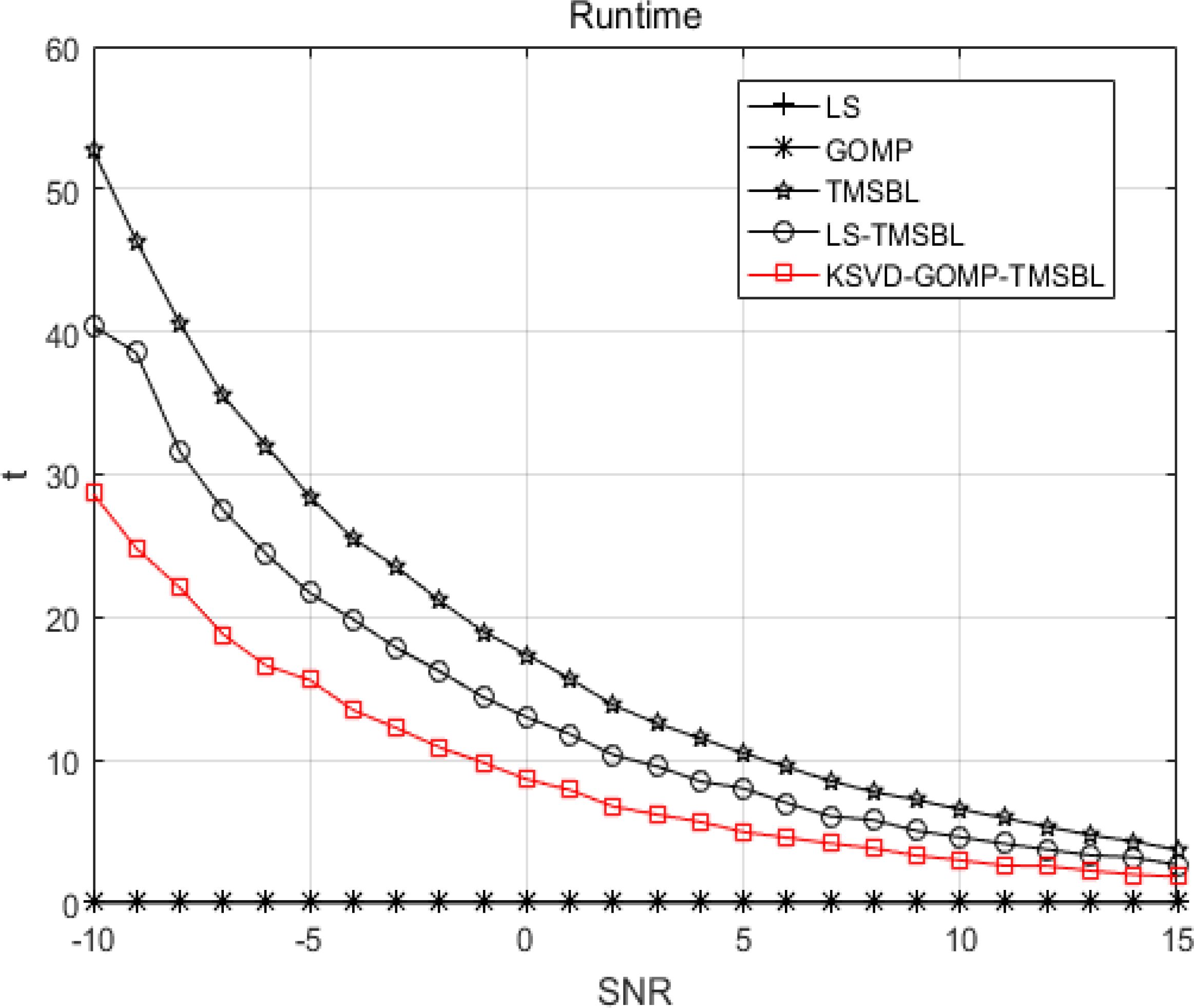
Figure 16. Running time of different channel estimation methods.

Table 3 illustrates the running time of various channel estimation methods under identical SNR conditions. As evident from Table 3, the running time of the KSVD-GOMP-TMSBL algorithm decreases in comparison to both the TMSBL and LS-TMSBL algorithms. At a signal-to-noise ratio of 0 dB, the running time of the KSVD-GOMP-TMSBL algorithm decreases by approximately 50.3% compared to TMSBL and 33.9% compared to LS-TMSBL algorithms. The running time of the KSVD-GOMP-TMSBL algorithm also decreases at different signal-to-noise ratio values. This indicates a reduction in the computational complexity of the KSVD-GOMP-TMSBL.

Table 3

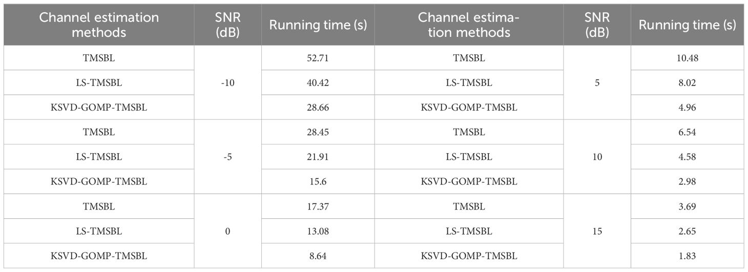
Table 3. Running time of different channel estimation methods.

5 Sea trial data validation

To validate the feasibility of the proposed algorithm, we utilized data obtained from sea trials in a specific maritime area for verification. For the offshore experiment, the sound source emission device UW350 was positioned at a depth of 5m. The pilot signal utilized was a 200-600Hz broadband long pulse signal with a sampling frequency of 10kHz, and the average in-band signal-to-noise ratio was -0.02dB. Based on GPS data, the distance between the transmitting ship and the receiving ship was calculated as 4672m. The receiving ship positioned the hydrophone in the seawater at a depth of 24m, and the depth of the experimental sea was measured at 25.5m. The depths of the mentioned equipment and seawater were measured by depth sensors.

Figure 17 depicts the channel estimation results obtained through the application of the KSVD-GOMP-TMSBL algorithm. The illustration reveals the relatively stable structure of the shallow-sea underwater acoustic channel, characterized by concentrated channel energy on a few paths, demonstrating sparse characteristics that manifest as a sparse multipath structure.

Figure 17

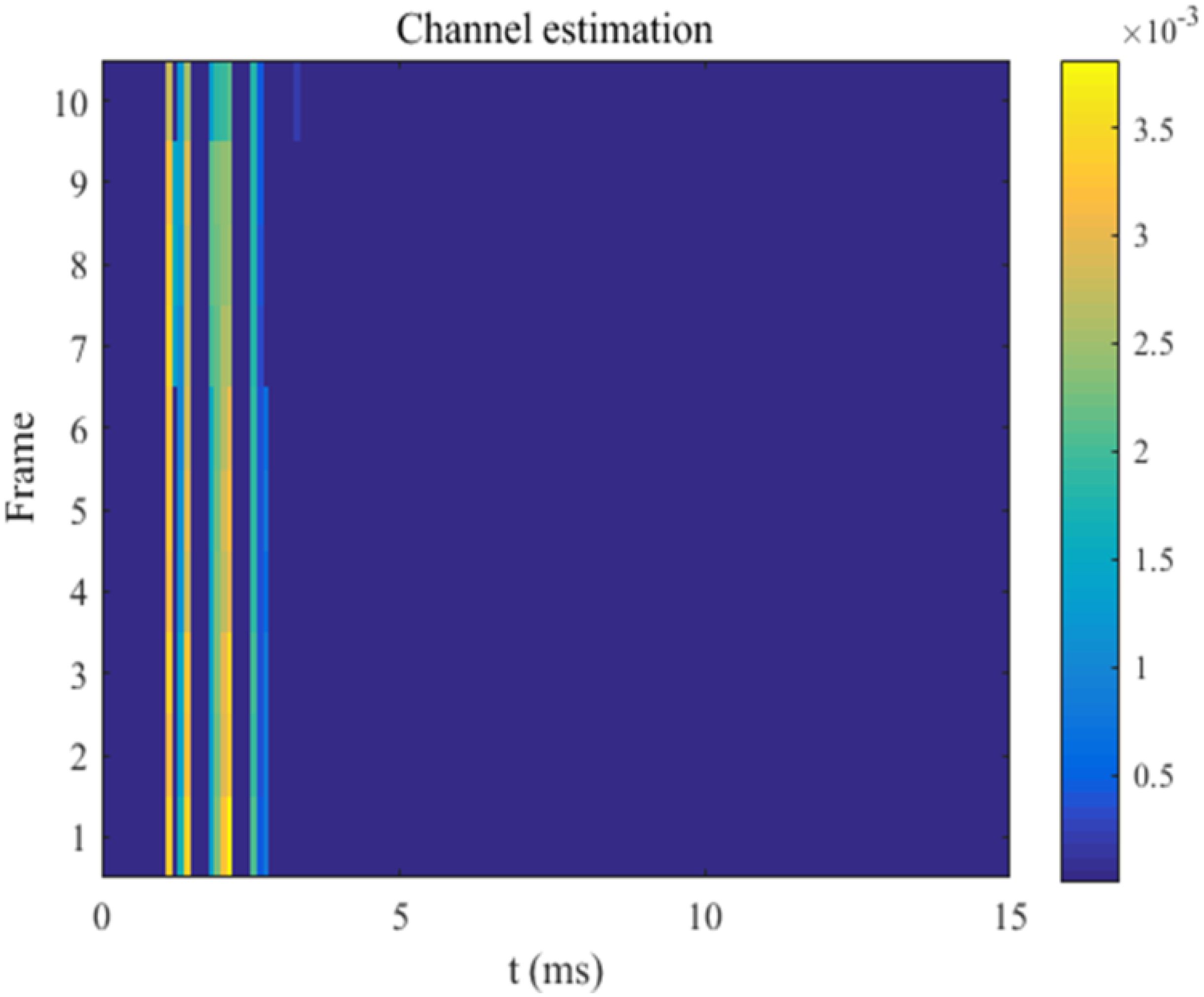
Figure 17. Channel estimation results.

Figure 18 illustrates the received BER for various channel estimation methods. The sparsity of the GOMP algorithm is set to 20, the energy coefficient of the LS-TMSBL algorithm is set to 0.05, and the sparsity of the KSVD-GOMP-TMSBL algorithm is set to 20, with an energy coefficient of 0.05. As depicted in Figure 16, the BER of the LS algorithm and GOMP algorithm is the highest among the considered algorithms. The LS algorithm is notably influenced by noise, leading to a high BER. Meanwhile, GOMP is extremely sensitive to sparsity, and the actual sparsity of the channel in the real environment is unknown, contributing to a high BER for the GOMP algorithm. The BER of both the TMSBL algorithm and the LS-TMSBL algorithm is lower than that of the LS algorithm and GOMP algorithm. In comparison to the aforementioned four algorithms, the BER of the KSVD-GOMP-TMSBL algorithm is lower, further validating its performance.

Figure 18

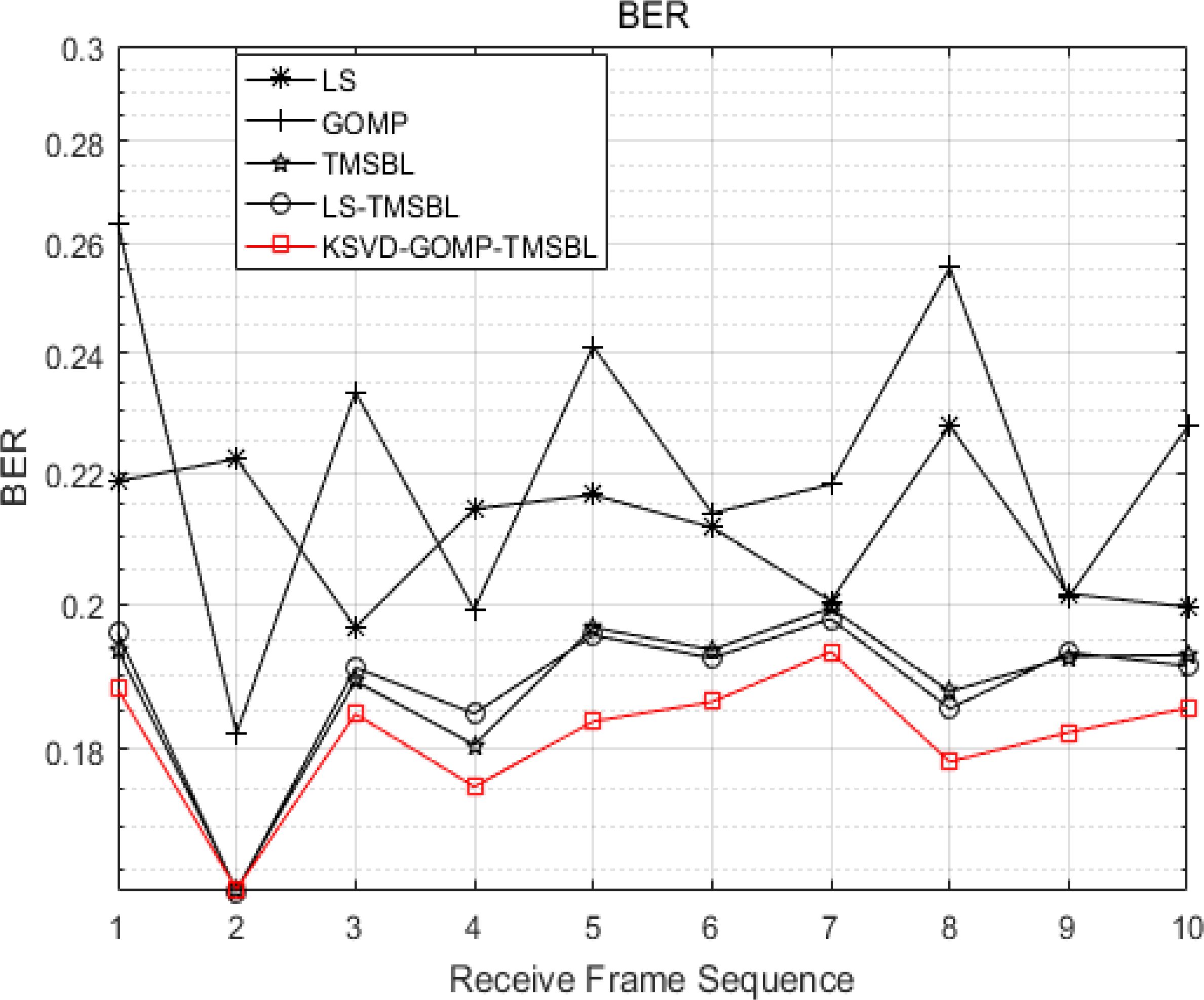
Figure 18. BER for different estimation methods.

Figure 19 depicts the runtime of different channel estimation methods. It is evident from the figure that the TMSBL algorithm and the LS-TMSBL algorithm have the longest runtime, approximately 15 seconds. The KSVD-GOMP-TMSBL algorithm boasts a runtime of approximately 11 seconds, marking a reduction of about 26.7% compared to the two preceding algorithms. The LS algorithm and the GOMP algorithm demonstrate the shortest running time; however, as shown in Figure 16, the KSVD-GOMP-TMSBL algorithm outperforms both the LS algorithm and the GOMP algorithm in terms of BER. The superiority of the KSVD-GOMP-TMSBL algorithm in running time is evident.

Figure 19

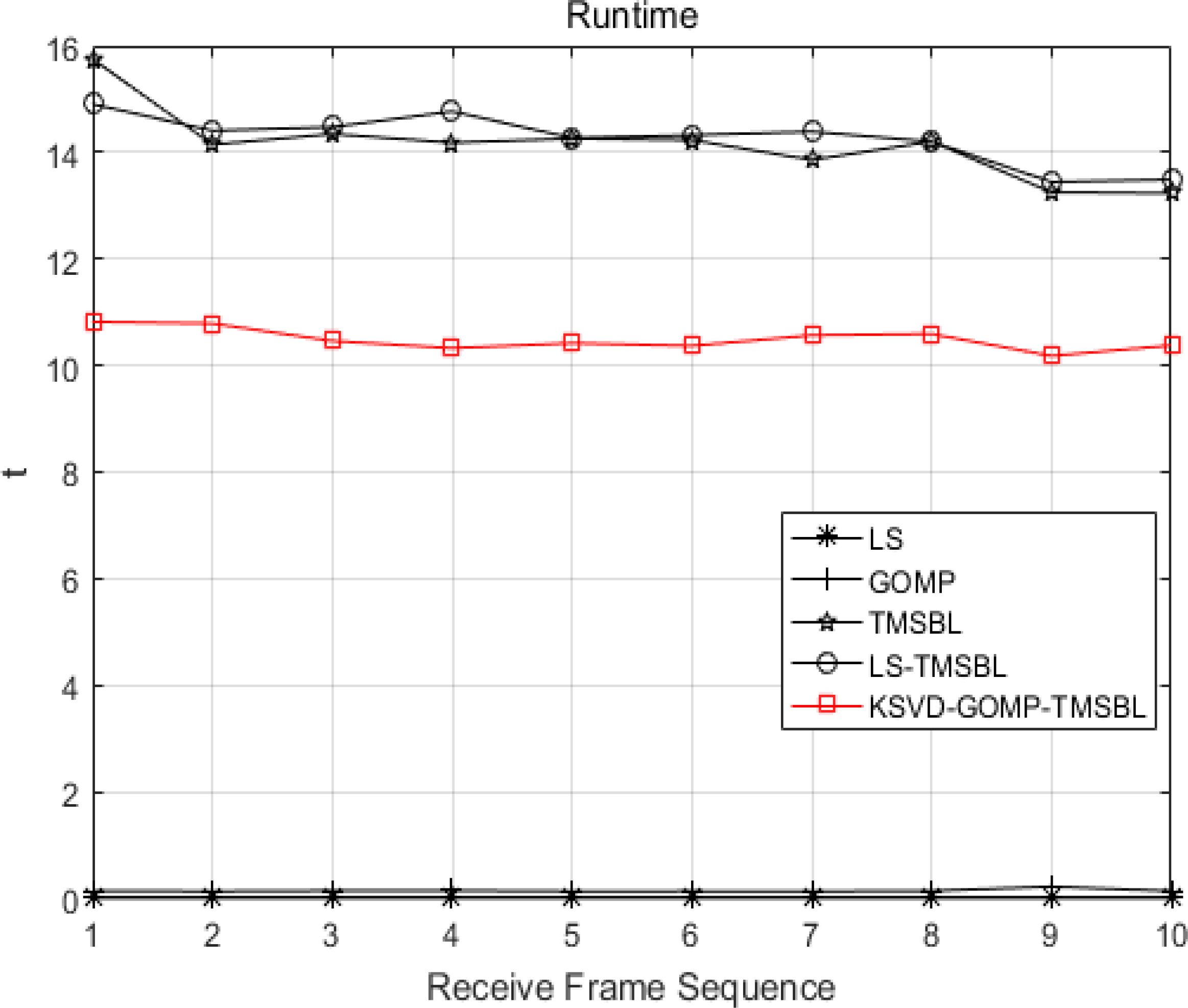
Figure 19. Running time of different channel estimation methods.

Table 4 provides the average BER and average runtime for different channel estimation methods. The average BER of different channel estimation methods is higher due to a lower average in-band SNR, and no channel coding is applied. However, it is evident that the KSVD-GOMP-TMSBL algorithm exhibits a lower average BER compared to the comparison algorithms. The KSVD-GOMP-TMSBL algorithm demonstrates the shortest runtime among the three channel estimation methods with a closer BER. This indicates that the KSVD-GOMP-TMSBL algorithm performs effectively in reducing both system BER and system complexity.

Table 4

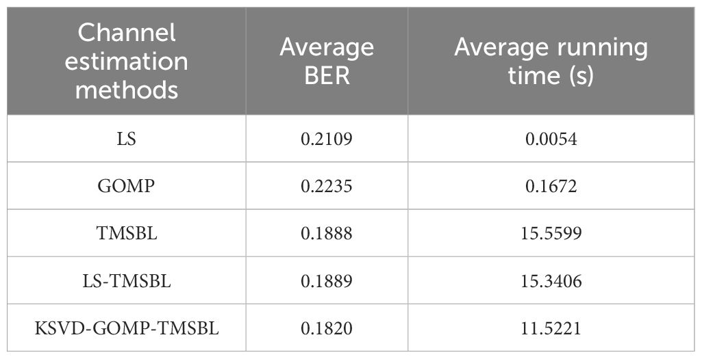
Table 4. Comparison of average BER and average runtime of different channel estimation methods.

6 Conclusion

The estimation of underwater acoustic channels using the TMSBL algorithm in shallow sea environments is challenged by high computational complexity, and the algorithm’s performance is significantly affected by the signal-to-noise ratio. The article proposes an improved channel estimation method for the temporal multiple sparse Bayesian learning OFDM underwater acoustic communication system. The K-SVD dictionary learning algorithm is employed to reduce noise in the received pilot matrix. Simultaneously, the null subcarrier is utilized to obtain a more accurate noise variance, thereby reducing the computational complexity of the algorithm and enhancing its noise immunity. The method employs the GOMP channel estimation algorithm to obtain the time-domain impulse response of the underwater acoustic channel. It acquires a priori knowledge of the TMSBL and selects the initial parameters of the EM algorithm based on the characteristics of the underwater acoustic channel, thereby enhancing the accuracy of channel estimation. Simulations indicate that at a signal-to-noise ratio of -10 dB, the KSVD-GOMP-TMSBL algorithm reduces the NMSE of channel estimation by 92.2% compared to the TMSBL algorithm, significantly improving estimation accuracy. Furthermore, the running time is reduced by 45.6%, thereby accelerating the convergence of the TMSBL algorithm and reducing its computational complexity. The validation with experimental data from the sea trials demonstrate that the proposed algorithm has a lower impact on the signal-to-noise ratio compared to traditional channel estimation algorithms, and exhibits strong robustness. It achieves accurate estimates even in low signal-to-noise conditions in shallow water and operates at high speed.

The KSVD-GOMP-TMSBL algorithm effectively addresses the problems associated with low estimation accuracy and high computational complexity in the estimation of acoustic channels in shallow water under the conditions of low signal to noise ratio. This algorithm serves as a reference for estimating the acoustic channel in shallow water. Although the algorithm can effectively improve the performance of channel estimation, the reliance on pilot signals means that their quantity will influence the algorithm’s performance. Therefore, the next step is to explore channel estimation methods that require fewer pilot signals to further enhance robustness.

Data availability statement

The original contributions presented in the study are included in the article/supplementary material. Further inquiries can be directed to the corresponding author.

Author contributions

CX: Writing – review & editing, Writing – original draft. YR: Writing – original draft, Writing – review & editing. ML: Writing – review & editing. GT: Writing – review & editing. QM: Writing – review & editing.

Funding

The author(s) declare financial support was received for the research, authorship, and/or publication of this article. This work was supported by the National Natural Science Foundation of China under Grant (61761048), the Basic Research Special General project of Yunnan Province, China (202101AT070132) and Yunnan Minzu University Graduate Research Innovation Fund Project (2024SKY122).

Conflict of interest

The authors declare that the research was conducted in the absence of any commercial or financial relationships that could be construed as a potential conflict of interest.

Publisher’s note

All claims expressed in this article are solely those of the authors and do not necessarily represent those of their affiliated organizations, or those of the publisher, the editors and the reviewers. Any product that may be evaluated in this article, or claim that may be made by its manufacturer, is not guaranteed or endorsed by the publisher.

References

Aharon M., Elad M., Bruckstein A. (2006). K-SVD: An algorithm for designing overcomplete dictionaries for sparse representation. IEEE Trans. Signal Process. 54, 4311–4322. doi: 10.1109/TSP.2006.881199

Crossref Full Text | Google Scholar

Chen P., Guo Q., Li P., Cui F. (2020). Joint sparse channel estimation and data detection based on bayesian learning in OFDM system. Comput. Sci. 47 (11A), 349–353. doi: 10.11896/jsjkx.191100090

Crossref Full Text | Google Scholar

Chen S. S., Donoho D. L., Saunders M. A. (2001). Atomic decomposition by basis pursuit. SIAM Rev. 43, 129–159. doi: 10.1137/S003614450037906X

Crossref Full Text | Google Scholar

Cheng H. K., Wang H. X. (2022). Time varying underwater acoustic channel estimation based on Kalman filter. Tech. Acoustics 41, 833–837. doi: 10.16300/j.cnki.1000-3630.2022.06.007

Crossref Full Text | Google Scholar

Cotter S. F., Rao B. D. (2002). Sparse channel estimation via matching pursuit with application to equalisation. IEEE Trans. Commun. 50, 374–377. doi: 10.1109/26.990897

Crossref Full Text | Google Scholar

Giao G., Song Q. J., Ma L., Liu S. Z., Sun Z. X., Gan S. W. (2018). Sparse Bayesian learning for channel estimation in time-varying underwater acoustic OFDM communication. IEEE Access 6, 56675–56684. doi: 10.1109/ACCESS.2018.2873406

Crossref Full Text | Google Scholar

Hong D. Y., Wang W., Yin L., Pu Z. Q., Zhou C. Y., Huang H. N. (2022). An improved temporal multiple sparse Bayesian learning under-ice acoustic channel estimation method. Acta Acustica 47 (5), 591–602. doi: 10.15949/j.cnki.0371-0025.2022.05.013

Crossref Full Text | Google Scholar

Jia S. Y., Zou S. C., Zhang X. C., Tian D. Y. (2022). Multi-block Sparse Bayesian learning channel estimation for OFDM underwater acoustic communication based on fractional Fourier transform. Appl. Acoustics 192, 108721. doi: 10.1016/j.apacoust.2022.108721

Crossref Full Text | Google Scholar

Jiang W. H., Tong F., Zhang H. T., Li B. (2021). Dynamic discriminative compressed sensing estimation of hybrid sparse underwater acoustic channel. Acta Acustica 46 (6), 825–834. doi: 10.15949/j.cnki.0371-0025.2021.06.005

Crossref Full Text | Google Scholar

Lyu X. R., Li Y. M., Guo Q. (2021). Joint channel and impulsive noise estimation method for MIMO-OFDM systems. J. Commun. 42, 54–64. doi: 10.11959/j.issn.1000–436x.2021238

Crossref Full Text | Google Scholar

Meng X. Y., Liu Z. L. (2023). TB-GOMP channel estimation algorithm for shallow underwater acoustic communication. J. Ordnance Equip. Eng. 44, 223–229. doi: 10.11809/bqzbgcxb2023.05.032

Crossref Full Text | Google Scholar

Tibshirani R. (1996). Regression shrinkage and selection via the lasso. J. R. Stat. Soc. Ser. B: Stat. Method. 58, 267–288. doi: 10.1111/j.2517-6161.1996.tb02080.x

Crossref Full Text | Google Scholar

Tong F., Wu F. Y., Zhou Y. H. (2022). Underwater acoustic channel estimation (China: Science Press).

Google Scholar

Wang H., Sun T. J., Liu T. (2020). Active sonar target classification based on dictionary learning. Tech. Acoustics 39 (5), 552–558. doi: 10.16300/j.cnki.1000-3630.2020.05.006

Crossref Full Text | Google Scholar

Wipf D. P., Rao B. D. (2004). Sparse Bayesian learning for basis selection. IEEE Trans. Signal Process. 52, 2153–2164. doi: 10.1109/TSP.2004.831016

Crossref Full Text | Google Scholar

Wipf D. P., Rao B. D. (2007). An empirical Bayesian strategy for solving the simultaneous sparse approximation problem. IEEE Trans. Signal Process. 55, 3704–3716. doi: 10.1109/TSP.2007.894265

Crossref Full Text | Google Scholar

Wu F. Y., Tong F. (2017). Improved compressed sensing estimation of block sparse underwater acoustic channel. Acta Acustica 42, 27–36. doi: 10.15949/j.cnki.0371-0025.2017.01.004

Crossref Full Text | Google Scholar

Xing C., Dong S., Wan Z. (2023). Direction-of-arrival estimation based on sparse representation of fourth-order cumulants. IEEE Access 11, 128736–128744. doi: 10.1109/ACCESS.2023.3332991

Crossref Full Text | Google Scholar

Xing C. X., Wang Z. L., Jiang S. Y., Yu R. M. (2022). Direction of arrival estimation based on high-order cumulant by sparse reconstruction of underwater acoustic signals. Acta Acustica 47, 440–450. doi: 10.15949/j.cnki.0371-0025.2022.04.010

Crossref Full Text | Google Scholar

Xing C. X., Wu Y. W., Xie L. X., Zhang D. Y. (2021a). A sparse dictionary learning-based denoising method for underwater acoustic sensors. Appl. Acoustics 180, 108140. doi: 10.1016/j.apacoust.2021.108140

Crossref Full Text | Google Scholar

Xing C. X., Zhang D. Y., Song Y., Wu Y. W., Xie L. X. (2021b). Research on inversion of sound speed profile using dictionary learning method. Tech. Acoustics 40 (6), 750–756. doi: 10.16300/j.cnki.1000-3630.2021.06.002

Crossref Full Text | Google Scholar

Xu W., Yan S. F., Ji F., Chen J. D., Zhang J., Zhao H. F., et al. (2016). Marine information gathering, transmission, processing, and fusion: current status and future trends. Scientia Sinica(Informationis) 46 (8), 1053–1085. doi: 10.1360/N112016-00064

Crossref Full Text | Google Scholar

Yang P. (2023). An imaging algorithm for high-resolution imaging sonar system. Multimed Tools Appl. 83, 31957–31973. doi: 10.1007/s11042-023-16757-0

Crossref Full Text | Google Scholar

Yin J. W., Gao X. B., Han X., Zhang X., Wang D. Y., Zhang J. C. (2021). Underwater acoustic channel estimation and impulsive noise mitigation based on sparse Bayesian learning. Acta Acustica 46 (6), 813–824. doi: 10.15949/j.cnki.0371-0025.2021.06.004

Crossref Full Text | Google Scholar

Zhang X. (2023). An efficient method for the simulation of multireceiver SAS raw signal. Multimed Tools Appl. 83, 37351–37368. doi: 10.1007/s11042-023-16992-5

Crossref Full Text | Google Scholar

Zhang X. B., Yang P. X., Wang Y. M., Shen W. Y., Yang J. C., Wang J. F., et al. (2024). A novel multireceiver SAS RD processor. IEEE Trans. Geosci. Remote Sens. 62, 1–11. doi: 10.1109/TGRS.2024.3362886

Crossref Full Text | Google Scholar

Zhang X., Wu H., Sun H., Ying W. (2021). Multireceiver SAS imagery based on monostatic conversion. IEEE J. Selected Topics Appl. Earth Observations Remote Sens. 14, 10835–10853. doi: 10.1109/JSTARS.2021.3121405

Crossref Full Text | Google Scholar

Zhang Z., Rao B. D. (2011). Sparse signal recovery with temporally correlated source vectors using sparse Bayesian learning. IEEE J. Selected Topics Signal Process. 5, 912–926. doi: 10.1109/JSTSP.2011.2159773

Crossref Full Text | Google Scholar

Zhu L., Liu S., Cao S. N., Liu Y. Y. (2020). Nonparametric Bayesian dictionary learning in sparse gradient domain for image denoising. Comput. Eng. Design 41 (3), 802–807. doi: 10.16208/j.issn1000-7024.2020.03.032

Crossref Full Text | Google Scholar