Investigating the influence of sub-mesoscale current structures on Baltic Sea connectivity through a Lagrangian analysis

This study explores the impact of sub-mesoscale structures and vertical advection on the connectivity properties of the Baltic Sea using a Lagrangian approach. High-resolution flow fields from the General Estuarine Transport Model (GETM) were employed to compute Lagrangian trajectories, focusing on the influence of fine-scale structures on connectivity estimates. Six river mouths in the Baltic Sea served as initial positions for numerical particles, and trajectories were generated using flow fields with varying horizontal resolutions: 3D trajectories with 250m resolution as well as 2D trajectories with 250m and 1km resolutions. Several Lagrangian indices, such as mean transit time, arrival depths, and probability density functions of transit times, were analyzed to unravel the complex circulation of the Baltic Sea and highlight the substantial impact of sub-mesoscale structures on numerical trajectories. Results indicate that in 2D simulations, particles exhibit faster movement on the eastern side of the Gotland Basin in high-resolution compared to coarse-resolution simulations. This difference is attributed to the stronger coastal current in high-resolution compared to coarse-resolution simulations. Additionally, the study investigates the influence of vertical advection on numerical particle motion within the Baltic Sea, considering the difference between 3D and 2D trajectories. Findings reveal that denser water in the eastern and south-eastern areas significantly affects particle dispersion in 3D simulations, resulting in increased transit times. Conversely, regions in the North-western part of the basin accelerate particle movement in 3D compared to the 2D simulations. Finally, we calculated the average residence time of numerical particles exiting the Baltic Sea through the Danish strait. Results show an average surface layer residence time of approximately 790 days over an eight-year integration period, highlighting the relatively slow water circulation in the semi-enclosed Baltic Sea basin. This prolonged residence time emphasizes the potential for the accumulation of pollutants. Overall, the study underscores the pivotal role of fine-scale structures in shaping the connectivity of the Baltic Sea, with implications for understanding and managing environmental challenges in this unique marine ecosystem.

1 Introduction

1.1 An overview of the application of the Lagrangian approach in oceanic connectivity analysis

The utilization of Lagrangian frameworks offers a powerful approach to quantifying and characterizing the intricate transport and connectivity patterns of water parcels across diverse temporal and spatial scales (Roughgarden et al., 1988; Kinlan and Gaines, 2003; Largier, 2003; Siegel et al., 2003; Cristiani et al., 2021; Drouet et al., 2021; Bharti et al., 2022; Hariri et al., 2022). This methodology enables a comprehensive assessment of crucial processes such as the dispersal of marine larvae, the dissemination of pollutants, and the exchange of genetic material among distinct populations. Moreover, Lagrangian methods offer a unique capability to explore connectivity in three dimensions, encompassing not only horizontal transport but also vertical dispersion. The three-dimensional perspective afforded by Lagrangian frameworks facilitates a comprehensive exploration of the intricate interactions between water masses, allowing for a more accurate representation of the prevailing connectivity patterns in diverse marine environments.

One of the key advantages of Lagrangian analysis lies in its ability to capture the inherent variability and complexity of ocean currents. This approach takes into account the individual paths of water parcels, thus considering the effects of mesoscale eddies, coastal jets, upwelling, and other localized flow phenomena (Poulain and Niiler, 1989; Swenson and Niiler, 1996; Blanke and Raynaud, 1997; Dever et al., 1998; LaCasce, 2008; Alberto et al., 2011; Watson et al., 2011; Mora et al., 2012; Van Sebille et al., 2012; Poulain and Hariri, 2013; Hariri et al., 2015; Hariri, 2020; Hariri, 2022; Van Sebille et al., 2018). These fine-scale processes exert a significant influence on connectivity patterns, thereby shaping the distribution of marine organisms, the dispersal of larvae, and the transport of contaminants (Dong and McWilliams, 2007; Dong et al., 2009; Mitarai et al., 2009).

In recent years, the application of Lagrangian methods in oceanography has led to profound insights into connectivity processes (Cristiani et al., 2021; Drouet et al., 2021; Bharti et al., 2022; Hariri et al., 2022). It has provided a more nuanced understanding of the mechanisms driving population dynamics, species distributions, and the spread of contaminants in the marine environment. The integration of Lagrangian analysis with remote sensing data and numerical models has further enhanced our ability to quantify and predict connectivity patterns in the ocean (Poulain and Niiler, 1989; Swenson and Niiler, 1996; Blanke and Raynaud, 1997; Dever et al., 1998; LaCasce, 2008; Mora et al., 2012; Poulain and Hariri, 2013; Hariri et al., 2015; Van Sebille et al., 2018). Overall, Lagrangian methods have facilitated the study of connectivity in oceanography, enabling us to unravel the intricate interplay between physical processes and ecological dynamics (Drouet et al., 2021; Ser-Giacomi et al., 2021; Wang et al., 2019). By embracing this approach, we can attain a more profound comprehension of the complex web of interactions that shape the functioning and resilience of marine ecosystems, ultimately informing sustainable management strategies and conservation efforts.

1.2 Description of the study area

The Baltic Sea, a distinctive water body in Northern Europe, is a complex hydrodynamic system shaped by a multitude of factors (Figure 1). These unique flow fields are the result of interactions between geographical features, atmospheric conditions, freshwater input, and the complex interplay of different water masses. Surface circulation, a prominent feature of the Baltic Sea, is primarily steered by wind patterns and atmospheric pressure systems. Prevailing winds, including the westerlies and polar easterlies, exert their influence, orchestrating surface currents. The strength and direction of these wind-driven currents exhibit seasonal variations and give rise to phenomena such as coastal upwelling (Lehmann and Myrberg, 2008) and downwelling systems (Emelyanov, 1995; Meier, 2007; Lass and Matthäus, 2008; Omstedt et al., 2014). Inflow and outflow dynamics play a crucial role in the Baltic Sea’s flow fields. Notably, the inflow of saline water from the North Sea through the Danish straits, like the Kattegat and the Sound, introduces saltier waters, impacting both salinity and circulation (e.g., Mohrholz, 2018). Conversely, the influx of freshwater from various rivers, such as the Vistula and the Neva, leads to a brackish water outflow into the North Sea (Winsor et al., 2001; Meier, 2007; Leppäranta and Myrberg, 2009; 2003). The Baltic Sea’s vertical stratification is a defining characteristic, stemming from differences in water density. Freshwater from river runoff, being less dense than the saltwater from the North Sea inflow, results in a layered structure, with fresher water at the surface and saltier, denser water at greater depths. This stratification is fundamental in shaping the movement of water masses, influencing nutrient cycling, and determining the distribution of marine life (Leppäranta and Myrberg, 2009; Uurasjärvi et al., 2021; Lehmann et al., 2022). The Baltic Sea’s flow patterns vary seasonally, with freezing in some areas during winters and stratification with thermocline development in summers (Stramska et al., 2013). Complex coastlines, islands, and the Coriolis effect further influence flow patterns, causing currents to deflect to the right in the Northern Hemisphere (Lehmann et al., 2002; Reissmann et al., 2009; Yi et al., 2013).

Figure 1

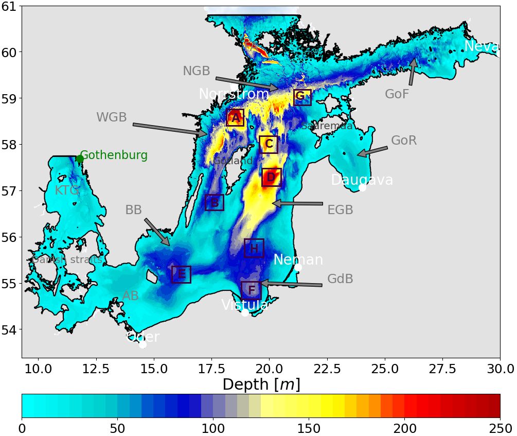
Figure 1 The nested model domain in the simulations. The location of the open boundaries (black lines), and abbreviations for different basins (AB, Arkona Basin; BB, Bornholm Basin; GdB, Gdansk Basin; EGB, Eastern Gotland Basin; NGB, Northern Gotland Basin; WGB, Western Gotland Basin; GoR, Gulf of Riga; GoF, Gulf of Finland) are shown. Black square boxes show the location of destination sites (defined based on the bathymetry of the Baltic Sea) for connectivity network analysis.

Understanding these flow patterns is crucial for navigation, environmental preservation, and ecological research. Oceanographers use various methods, like numerical models and Lagrangian approaches, to explore water movement and particle dispersion in the Baltic Sea as an important marine environment, with particular relevance due to its unique characteristics and challenges. Various prior studies have employed Lagrangian particles in the Baltic Sea for diverse purposes, including analyzing meridional overturning circulation (Döös et al., 2004), investigating particle dispersion with surface drifters and modeled trajectories (Kjellsson and Döös, 2012), mitigating environmental risks from the marine industry by assessing pollution transport (oil spills) (Soomere et al., 2014), studying particle transport between coastal areas using high-resolution trajectory modeling (Corell and Döös, 2013), refining model trajectories and dispersion rates with surface drifter observations (Kjellsson et al., 2013), investigating connectivity analysis (Corell et al., 2012; Teacher et al., 2013; Sjöqvist et al., 2015; Jonsson et al., 2020), examining eddy characteristics in the southern Baltic Sea (Zhurbas et al., 2019), exploring Lagrangian Coherent Structures and hypoxia in the Baltic Sea (e.g., Giudici et al., 2021; Dargahi, 2022), simulating marine macro-plastic transport and distribution in the Baltic Sea (Christensen et al., 2023), and detecting transport barriers using Lagrangian descriptors with applications to the Baltic Sea (Vortmeyer-Kley et al., 2016), among others. In recent years, the impact of sub-mesoscale processes on the temperature and salinity distribution in the Baltic Sea has been studied. Processes characterized by the Rossby and Richardson number in the order of 1 (e.g. Thomas et al., 2008; McWilliams, 2016) and horizontal length scales on the order of 1 km can be considered sub-mesoscale. High-resolution observations (e.g. Lips et al., 2016; Salm et al., 2023) and modelling (e.g. Väli et al., 2017; Onken et al., 2020; Chrysagi et al., 2021) have been used to characterize and analyze the presence of sub-mesoscale features in the Baltic Sea.

1.3 The aim of the study

Previous Lagrangian studies have made significant contributions to addressing specific challenges and management issues in the Baltic Sea region (e.g., Corell et al., 2012; Teacher et al., 2013; Sjöqvist et al., 2015; Roiha et al., 2018; Jonsson et al., 2020). However, these studies were based upon coarse-resolution flow field data because sub-mesoscale permitting and mesoscale resolving model simulations were lacking.

Furthermore, a considerable portion of previous studies investigating connectivity in ocean flows has tended to concentrate on the surface layer (e.g., Cristiani et al., 2021; Drouet et al., 2021; Bharti et al., 2022; Hariri et al., 2022). Considering these limitations, the objective of this study is to analyze the connectivity properties of the Baltic Sea through the application of Lagrangian techniques and freshwater particles. We conduct a comprehensive analysis using output data from various resolutions of a flow field of an Ocean General Circulation Model (OGCM). In this paper, we examine transport and dispersion in the Baltic Sea.

i. We aim to understand the degree of connectivity among particles from different rivers representing various coastal sections in the Baltic Sea.

ii. We are interested in exploring how the trajectories of freshwater particles in the Baltic Sea differ when either 2D or 3D dynamics are considered.

iii. We determine the time it takes for particles originating from the coastal zone to reach the interior sub-basins of the Baltic Sea and investigate the role of sub-mesoscale structures and mesoscale eddies in their dispersal.

iv. We investigate the residence times of freshwater particles, both within the sea surface layer and without any restrictions.

2 Data and methods

We investigate the influence of sub-mesoscale structures and vertical advection by comparing connectivity estimates derived from high-resolution velocity fields in the Baltic Sea. These velocity fields are generated using the high-resolution General Estuarine Transport Model (GETM; Burchard and Bolding Kristensen, 2002). To perform our analysis, we are conducting offline Lagrangian transport experiments by releasing numerical particles from multiple distributed locations, specifically river mouths, within the study region.

2.1 Numerical model

GETM is a hydrostatic, three-dimensional primitive equation model that has embedded adaptive vertical coordinates (Hofmeister et al., 2010; Gräwe et al., 2015). Combined with the total variance diminishing (TVD) advection scheme and the Superbee limiter, GETM significantly reduces numerical mixing in the simulations (Klingbeil et al., 2018). The vertical mixing in the GETM is calculated via coupling with the GOTM (General Ocean Turbulence Model; Burchard and Bolding, 2001) and more precisely, a two-equation k-epsilon scheme with an algebraic closure of the second moment (Canuto et al., 2001) has been selected. The horizontal mixing (viscosity and diffusion) is calculated using a Smagorinsky parameterisation (Smagorinsky, 1963).

A high-resolution nested model version (HR2D-250m and HR3D-250m) was constructed for the main part of the Baltic Sea comprising the Arkona Basin (AB), the Bornholm Basin (BB), the Gdansk Basin (GdB), the Eastern Gotland Basin (EGB), the Northern Gotland Basin (NGB), the Western Gotland Basin (WGB), the Gulf of Riga (GoR), and the Gulf of Finland (GoF) (see Figure 1). In the model domain, the horizontal grid spacing was 250 m. Sixty vertically adaptive layers were used. The maximum layer thicknesses in the two uppermost layers were limited to 0.5 m.

A 9-year simulation from 2010 to 2018 was carried out. Open boundaries with a one-way nesting approach were used in the western and northern part of the model domain. At the lateral boundaries, results from a 1 nautical mile (approximately 1852 m) Baltic Sea model with 1-hourly resolution for sea surface height and 3-hourly resolution for salinity, temperature and current profiles were spatially and temporally interpolated onto the grid of the high-resolution model. The coarse resolution model run started on 01.04.2009 and used the Copernicus Marine Service reanalysis product “BALTICSEA_REANALYSIS_PHYS_003_008” for the initial conditions of temperature and salinity. The details of the coarse resolution model can be found in Radtke et al. (2020) and Väli et al. (2023), respectively.

The momentum and heat fluxes were calculated from the output of the regional reanalysis data set UERRA-HARMONIE with a spatial resolution of 11 km and a temporal resolution of 1 hour. The long-term, high-quality and high-resolution dataset was originally produced within the FP7 project UERRA (Uncertainties in Ensembles of Regional Re-Analyses, http://www.uerra.eu/) and is part of the Copernicus Climate Change Service (C3S, https://climate.copernicus.eu/copernicus-regional-reanalysis-europe) (Gröger et al., 2022).

The freshwater input to the Baltic Sea came from the dataset produced for the BMIP (Baltic Model Intercomparison Project; Gröger et al., 2022) based on the E-HYPE (Lindström et al., 2010) hindcast and forecast products (Väli et al., 2019). The total Baltic Sea dataset includes 91 rivers, while 56 rivers were used for the high-resolution model runs.

The high-resolution run started with initial conditions at rest where the sea surface height was set to zero. The initial temperature and salinity fields were taken at a vertical resolution of 10 m from the coarse-resolution model results for 30.12.2009 and interpolated to the high-resolution model grid. Adjustment of wind-driven currents is expected within 10 days (Krauss and Brügge, 1991; Lips et al., 2016), but geostrophic adjustment may take several years (Meier, 2007). For comparison with the high-resolution model version (HR2D-250m and HR3D-250m), a medium resolution setup (HR2D-1km) for the Baltic Sea based on GETM with horizontal grid spacing of 0.5 nautical miles (approximately 926 m) is used within the study. A detailed description of this configuration is given by Zhurbas et al. (2018) and Liblik et al. (2020, 2022). Model simulations and their setups are summarized in Table 1.

Table 1

Table 1 Summary of GETM setups used within this study.

The validation of the setups with the coarse and medium horizontal resolutions has been presented in numerous papers before. For instance, CR3D-2km has been validated by Gräwe et al. (2019) and Radtke et al. (2020) and HR2D-1kmby Zhurbas et al. (2018) and Liblik et al. (2020; 2022).

The validation of the high-resolution model, HR2D-250m/HR3D-250m, is presented in the Supplementary materials by Väli et al. (2023). They compared the observed and simulated sea surface heights in coastal stations around the model domain and had highest correlations and lowest biases in the eastern and central part of the sea, while the largest errors (both in correlation and biases) occurred close to the Danish straits. The comparison of salinity in offshore monitoring stations indicated larger overestimation in the surface and rather concurring values in bottom layers, while the temperature was overestimated in the southern part of the sea (AB and BB) and relatively close to observations in the central and northern part (EGB and NGB).

2.2 Methods

2.2.1 Simulation of trajectories

To study ocean connectivity in the Baltic Sea, Lagrangian numerical particles were released at six major river mouths. The selected rivers are characterized by large water discharge and a strategically chosen location to cover all coastal sections of the Baltic proper. The particle positions at each time step are calculated using OceanParcels (Lange and van Sebille, 2017), a three-dimensional Lagrangian particle tracking model that is compatible with many OGCM outputs. The model utilizes the Runge–Kutta method to interpolate velocity values and to move the particle over a user-defined time step, which was set to 10 minutes. The trajectory of each particle is calculated based on Equation 1:

$\begin{array}{ll}dx=U.dt& (1)\end{array}$

where x is the particle position, U is the flow field obtained by GETM and dt is the time step.

In each Lagrangian experiment, a total of 100,000 particles were released at each river mouth (Neva, Vistula, Neman, Oder, Daugava, and Norrström), resulting in 600,000 particles in total (Figure 1). This large number of particles was released to provide statistically more robust estimates. The particles were released at random initial times, and their trajectories were tracked for a minimum of one year. For 3D simulations, particles were released at various depths, ranging from the surface to the base of 20 m. The maximum integration time was set at eight (2011-2018) and three years (2011-2013) for 2D and 3D simulations, respectively.

To compare the results, three simulations were conducted (Table 2). The first simulation, HR3D-250m, involved trajectory simulations using high-resolution 3D velocity fields with a horizontal resolution of 250 m. The second simulation, HR2D-250m, involved trajectory simulations using high-resolution 2D velocity fields with a 250 m horizontal resolution in the surface layer. The third simulation, HR2D-1km, used high-resolution 2D velocity fields with a horizontal resolution of 1 km in the surface layer (Supplementary Figure S1).

Table 2

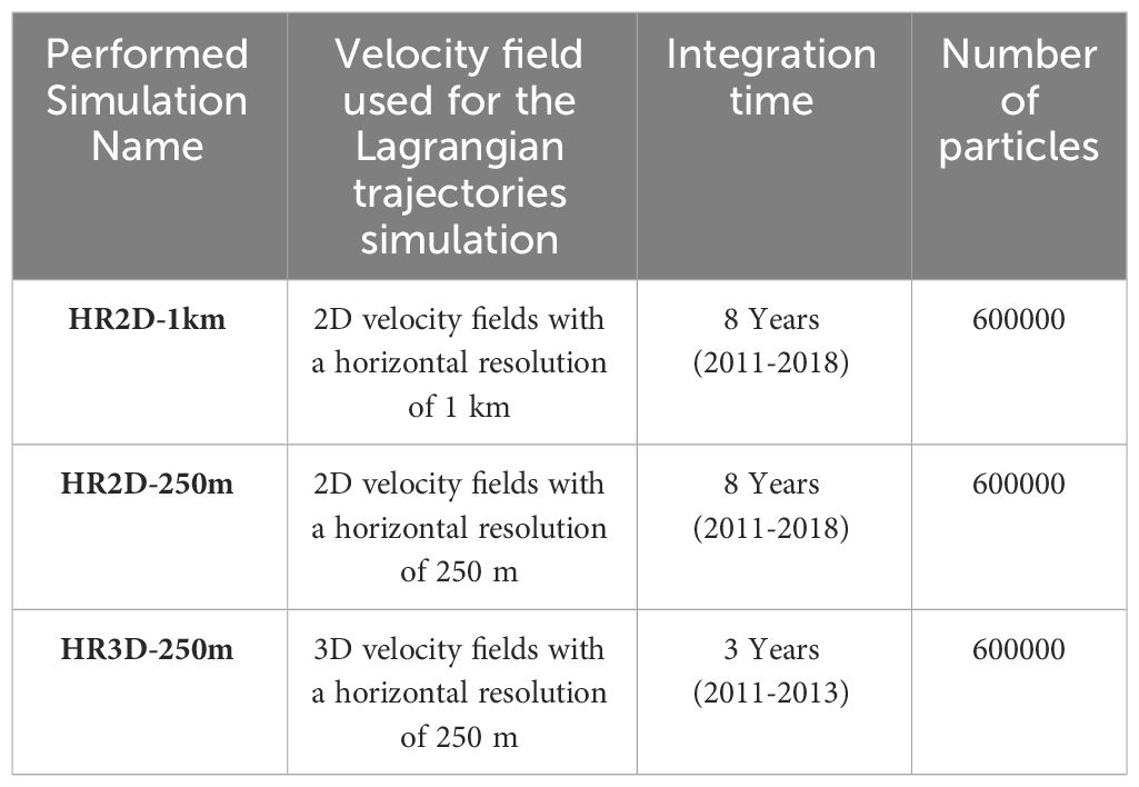
Table 2 Summary of the performed lagrangian simulations.

2.2.2 Lagrangian transit time and Lagrangian PDF

Transit time is a widely used method to quantify connectivity between marine sites through the tracking of passive Lagrangian particles. However, the traditional definition of “connectivity time” as the mean time it takes for particles to travel from one location to another is problematic in the global ocean, as every particle will eventually reach all areas of the domain over a long period. To overcome this issue, Jönsson and Watson (2016) introduced the “minimum connectivity time” (Min-T) concept, which represents the fastest travel time from source to destination for numerical particles. This method has been proven to align well with genetic dispersal in marine connectivity. In this study, we focus on the mean values of minimum connectivity (transit) time for all particles that move from one river mouth to the rest of the basin.

In addition to transit time, the Lagrangian PDF approach provides a more precise explanation and prediction of the particle dispersion process due to dispersion. This approach is commonly employed for turbulent flows (Pope, 1994) and provides the probability of particle movement from one location to another within a given time interval. However, obtaining accurate PDF values requires a significant number of trajectories as they estimate the mean dispersion properties of numerical particles. For our study, we deployed 100,000 particles at each examined river mouth, which is a sufficiently large number to provide connectivity estimates while still being computationally feasible. By using this method, we were able to obtain the Lagrangian PDF for particles released from each river mouth, as demonstrated in the study by Mitarai et al. (2009).

$\begin{array}{ll}LagrangianPDF(\xi ,t)=\frac{n_{\xi }(t)}{N*S_{\xi }}& (2)\end{array}$

where ξ is the sample space related to the discretion of Lagrangian PDF (here, a sample space of ∼ 0.25 km² is applied for the calculation of the PDF fields), S is the area of the sample space ξ, N is the total number of Lagrangian particles, and n_ξ(t) is the number of particles residing in the sample space ξ at the simulation time t.

2.2.3 Residence time

The residence time refers to the average time that a numerical particle spends in a particular basin. It is a vital factor for comprehending the behavior and fate of pollutants, contaminants, and essential nutrients in marine ecosystems. The duration of the residence time of particles can vary based on their location within the ocean. For instance, particles in shallow coastal regions have shorter residence times due to higher velocities and mixing, while particles in deep ocean regions have longer residence times due to slower currents and less mixing.

In this study, we computed the basin-average residence time of numerical particles as they exit the Baltic Sea through the Danish straits. Our aim was to gain a comprehensive understanding of their dispersion over a maximum advection period of eight years.

Furthermore, utilizing the decay rate (dissipation rate) of numerical particles over an eight-year duration, we were able to determine the cumulative residence time value for all particles exiting the basin in accordance with previous studies (Döös et al., 2004).

The normalized population in the basin, C(t), and its residence time, T, are defined by Buffoni et al. (1997) as follows:

$\begin{array}{ll}\complement (t)=\underset{\Omega }{\int }c(x,t)dx& (3)\end{array}$

$\begin{array}{ll}T=\underset{0}{\overset{\infty }{\int }}\complement (t^{\prime })dt\text{'}& (4)\end{array}$

where c(t, x) represents the average normalized tracer concentration at point x and time t (after a uniform initial release in the entire basin), and Ω represents the basin. C(t) and T can also be defined in the Lagrangian framework as:

$\begin{array}{ll}C(t)=\frac{N(t)}{N(0)}& (5)\end{array}$

$\begin{array}{ll}\underset{t\to \infty }{T=\text{lim}T}& (6)\end{array}$

$\begin{array}{ll}{T}^{}=\frac{tN(t)}{N(0)}+{\sum }_{i=1}^{N_e(t)}\frac{t_e(i)}{N(0)}& (7)\end{array}$

where N(0) is the number of tracer particles initially deployed in the basin, N(t) is the number of particles at time t, Ne is the number of particles that have already escaped the basin at time t, and te is the escape time of the ith particle.

3 Results

3.1 2D connectivity analysis

3.1.1 Surface connectivity: transit time

In this section, we compare the transit time values for numerical particles that were initially released from various river mouths in the Baltic Sea (Figures 2, 3). We examine the effects of sub-mesoscale structures on the movement of numerical particles on the surface layer of the Baltic Sea using two different high-resolution velocity fields.

Figure 2

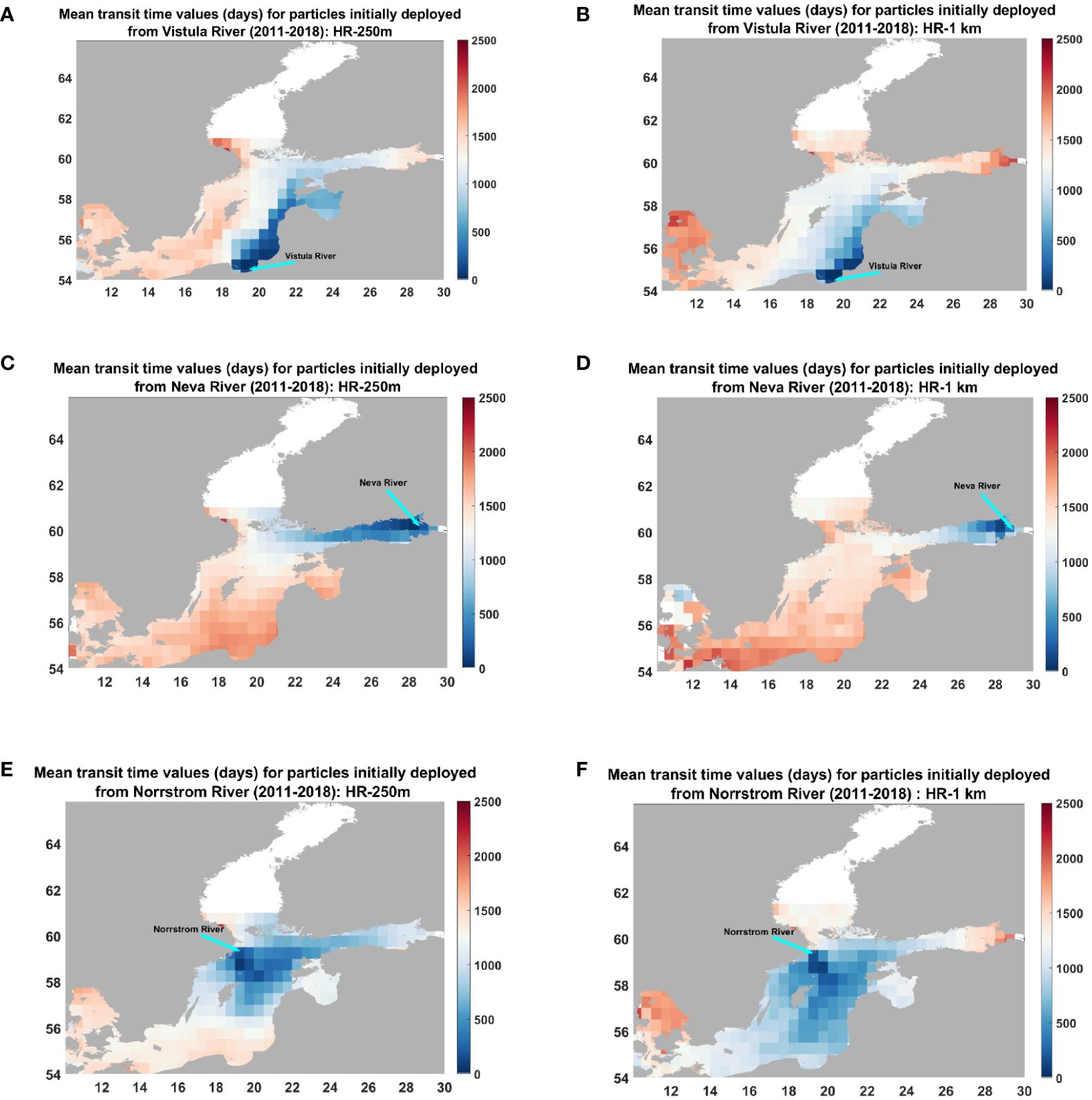
Figure 2 Comparison of mean transit time values during 2011-2018 on surface layer (2D): for particles initially deployed from Vistula River (A) HR-250m, (B) HR-1km; for particles initially deployed from Neva River (C) HR-250m, (D) HR-1km; and for particles initially deployed from Norrstrom River (E) HR-250m, (F) HR-1km.

Figure 3

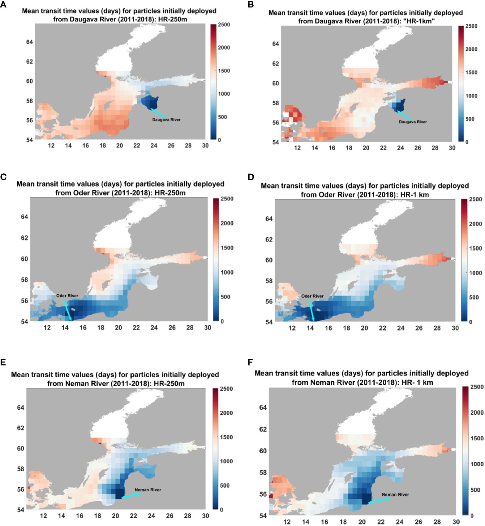
Figure 3 Comparison of mean transit time values during 2011-2018 on surface layer (2D): for particles initially deployed from Daugava River (A) HR-250m, (B) HR-1km; for particles initially deployed from Oder River (C) HR-250m, (D) HR-1km; and for particles initially deployed from Neman River (E) HR-250m, (F) HR-1km.

Figure 2 presents the transit time values of the numerical particles initially released from the Vistula River, located in the southern part of the Baltic Sea. Results from the higher resolution case (HR2D-250m) demonstrate that particles move much faster on the eastern side of the basin compared to the coarser resolution case (HR2D-1km). Thus, particles reach the Gulf of Finland in less than 1000 days in the higher resolution simulation, while it takes more than 1400 days in the coarser resolution case. Conversely, particles exit the Baltic Sea in approximately 1500 days in HR2D-250m, whereas they reach their final destination outside the Baltic Sea in less than 1300 days in HR2D-1km. This result implies that numerical trajectories simulated based on two different flow fields follow different pathways in the basin. The HR2D-250m simulation can better capture the small-scale turbulent features of the currents than the coarse-resolution HR2D-1km. Turbulent eddies and vortices can cause Lagrangian particles to exhibit more complex and meandering trajectories, sometimes leading to a slower motion, especially when viewed over short time intervals. In HR2D-250m, particles are more affected by the strong coastal currents on the eastern side of the basin, which propel them to move faster to the northern part of the Baltic. In the HR2D-1km case, particles tend to follow the surface return currents on the eastern and western parts of the Gotland Basin.

Additionally, results show significant differences in the value of transit times in the western part of the Baltic Sea obtained by HR2D-250m and HR2D-1km flow fields. Our findings elucidate that particles originating from the Vistula River reach the western part of basin in less than 1200 days in HR2D-1km, a value that extends to approximately 1500 days in HR2D-250m, considering that following coastal rim currents takes more time than the diffusive propagation across the Gotland Basin.

Additionally, we examined transit times of particles released from the Neva River (Figure 2). The results indicate that, due to the stronger coastal currents in the Gulf of Finland, particles arrive at the northern coasts of Gotland in HR2D-250m faster than in HR2D-1km, with a difference of approximately 300 to 500 days. Furthermore, particles from the Gulf of Finland tend to follow the currents on the western side of the Baltic Sea. Our findings show that the transit time from the Neva River to the southern parts of the basin, close to the Oder River, is about 1500 and 2000 days in HR2D-250m and HR2D-1km, respectively.

The behavior of particles released from the Norrström river (the river Norrström is the primary outlet of Lake Mälaren into the Baltic Sea), located at the western side of the basin, differs between the two simulations (Figure 2). In HR2D-250m, the particles follow two distinct pathways. One group moves towards the northern part of the basin, with some reaching the Gulf of Finland. After arriving close to the Åland Sea at the northern open boundary, the first group is influenced by return currents from the Gulf of Finland and then follows the current on the western part of the basin before exiting through the Arkona Basin. The second group follows the currents towards the eastern part of the Gotland Basin and is primarily directed towards the southern part of the basin because of the return currents in the eastern part of the Gotland Basin.

In the coarser resolution simulation, the particles from the Norrström river follow the general circulation patterns of the Baltic Sea on both the western and eastern sides of the Gotland Basin. The particles reach the Gulf of Riga faster in this case than in HR2D-250m. However, particles take longer to arrive at the Gulf of Finland in HR2D-1km. Additionally, the particles reach the southern part of the Baltic Sea faster in the coarser resolution simulation than in HR2D-250m, with a transit time difference of approximately 600 days (Figure 2).

The differing particle behavior along the southern part of the Swedish coast in the two simulation cases may be due to the higher number of eddies present in the HR2D-250m simulation, particularly in the northern part of the Gotland Basin. These eddies exhibit varying lifetimes and hold a notable influence in transporting and steering particles toward the upper sections of the basin. These swirling currents, with their varying durations, contribute to the particle trajectories that we observe, ultimately shaping the dynamics of particle movement in this area (please see finite time/size Lyapunov exponents fields in Supplementary Figure S2).

Furthermore, Figure 3 displays the transit time values for particles initially released from the other investigated rivers (Neman, Oder, and Daugava). The distribution of transit time values for particles initially deployed from the Oder River, in both simulations, exhibits a similar pattern, except on the western side of the Baltic Sea, where the motion in HR2D-1km is faster. Furthermore, particles deployed at the Neman River mouth follow similar patterns, except the motion in the southwestern part of the basin, near the exit areas, showing faster exit times for HR2D-1km, ranging between 300 to 500 days. Particles initially deployed from the Daugava River exhibit completely different behavior in both simulations. In HR2D-250m, particles move more rapidly towards the areas near the GOF, whereas in HR2D-1km, particles tend to move towards the western and eastern sides of the basin.

Figure 4 shows the connectivity matrices among areas in proximity to various river mouths. These matrices enable us to discern the intricate connection patterns among specified rivers. For instance, our findings unveil compelling insights into the transport dynamics of particles originating from the Gulf of Riga and the Gulf of Finland, shedding light on their arrival times at the Oder River. In HR2D-250m, these particles generally take approximately 1500 to 1550 days to arrive at the Oder River mouth. However, in HR2D-1km, the transit times extend to about 1750 to 1850 days. Intriguingly, particles originating from the Oder River exhibit diverse arrival times at these two gulfs, with particles reaching the Gulf of Riga and the Gulf of Finland in approximately 1200 and 1650 days, respectively.

Figure 4

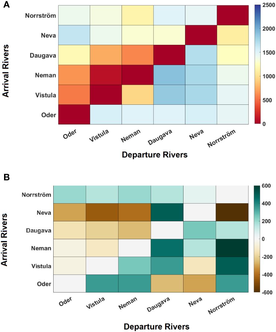
Figure 4 Connectivity matrices based on mean transit time values between selected rivers (A: mean transit time (days) for HR2D-250 m, B: mean transit time differences (days) between HR2D-250m and HR2D-1km).

The connection between the eastern and western sides of the basin can be established through network construction (Supplementary Figure S3). From the Norrström River to the Neman River, it takes approximately 1400 days in HR2D-250m, while this transit time is roughly halved to about 750 days in HR2D-1km. In the reverse direction, the transit time in HR2D-250m is 950 days, while in HR2D-1km, it is 700 days. The presence of sub-mesoscale structures in HR2D-250m, which are not resolved in HR2D-1km, influences the flow dynamics and transit times.

3.1.2 Surface connectivity: Lagrangian PDF

We examined the influence of fine-scale structures on numerical particle movement using Lagrangian probability density function (PDF, Equation 2) fields (Figures 5; Supplementary Figures S4, S5). The dispersion rates of the numerical particles were analyzed based on their PDF fields during different periods from their initial deployment. For the first six months, the numerical particles released from the Oder River in the southern part of the Baltic Sea remained close to their initial positions in both HR2D-250m and HR2D-1km. However, the HR2D-250m particles exhibited greater dispersion and moved further away than those in the coarser resolution case. The results indicated that particles tend to follow the large-scale mean circulation.

Figure 5

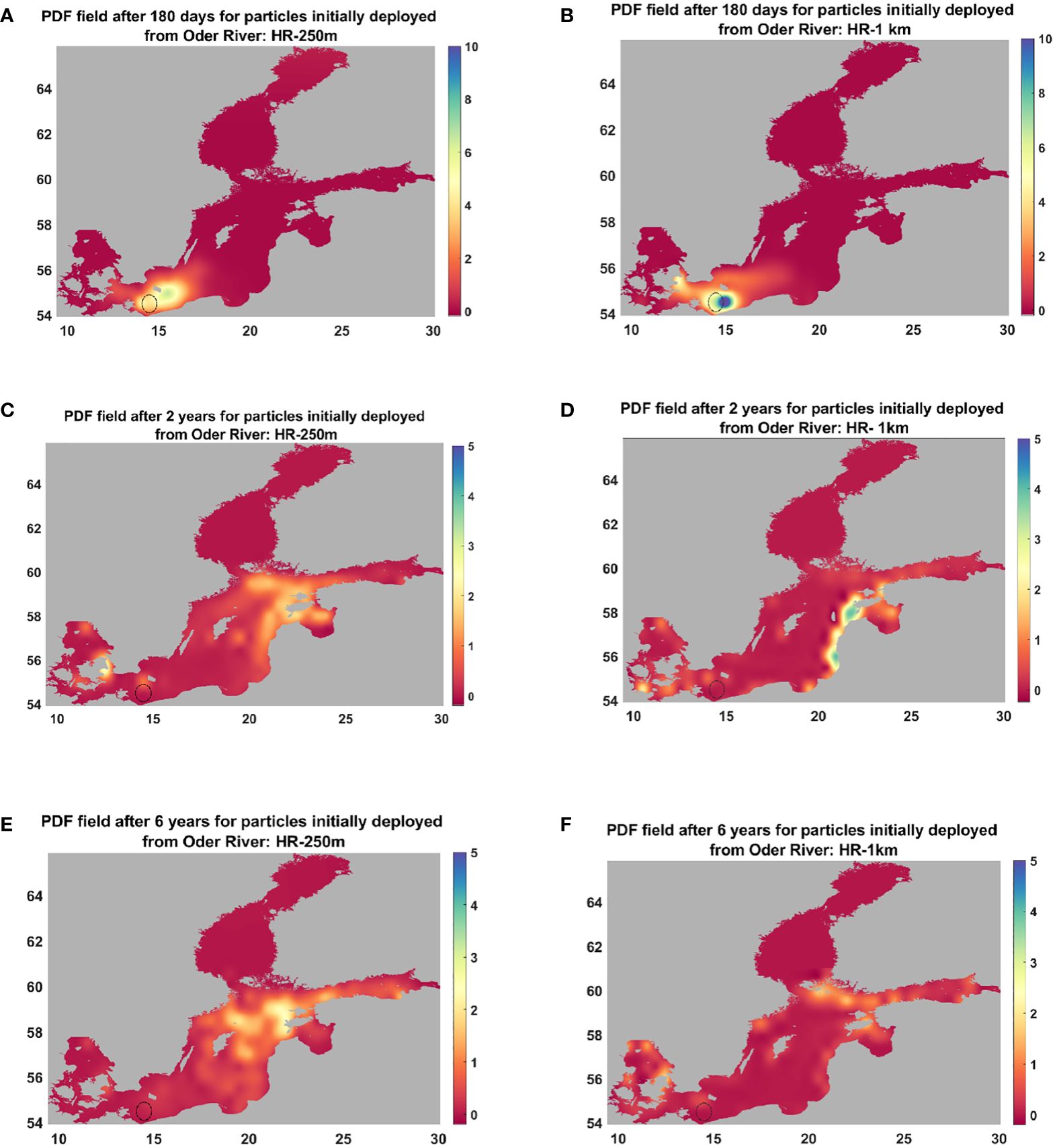
Figure 5 Lagrangian PDF field for particles initially deployed on the surface layer of the Baltic Sea from Oder River: after six months: (A) HR-250m, (B) HR-1km; after 2 years: (C) HR-250m, (D) HR-1km; and after 6 years: (E) HR-250m, (F) HR-1km.

After two years, the high dispersion dynamics generated by sub-mesoscale structures caused particles to cover significant parts of the eastern side of the Baltic Sea, close to the Gulf of Riga and the Gulf of Finland. In HR2D-1km, particles were affected by mean currents on the eastern side of the Baltic Sea and were concentrated in eastern coastal areas. Fewer particles had the possibility to enter the Gulf of Riga or the Gulf of Finland (Figure 5).

Six years after deployment, particles in HR2D-250m covered almost the entire basin, with more concentration on the northern, western, and eastern sides of the Gotland Basin and the southern part of the Baltic Sea. Conversely, in HR2D-1km, particles were less affected by dispersion, leading to more concentration along the Gulf of Finland and a portion of the Gulf of Riga.

3.2 3D connectivity analysis

3.2.1 Transit time comparison between 2D and 3D trajectories

Vertical advection plays an important role in the dynamics of the marine ecosystem in the permanently stratified Baltic Sea. Therefore, it is crucial to assess the impacts of vertical advection on the movement of numerical particles and compare the connectivity properties of different parts of the Baltic Sea in 3D and 2D simulations. In this section, we present detailed information on 3D Lagrangian connectivity analysis in the Baltic Sea, using numerical particles deployed in various river mouths as a starting point.

Figure 6 depicts transit time maps generated by 3D simulations of particles initially released from the Oder, Neman, and Norrström Rivers, as well as the differences in transit times between 3D and 2D simulations. The results show that particles originating from the Oder River take longer to reach different parts of the basin in the 3D simulation compared to the 2D simulation. Due to vertical dispersal, particles take approximately 550 days to arrive on the eastern side of the Baltic Sea in HR3D-250m, compared to about 450 days in HR2D-250m. A similar result is observed for particles arriving in the Gulf of Finland. The most significant differences in transit times are observed in the southern and eastern parts of the Baltic Sea, while in the western part differences in travel time between trajectories in 3D and 2D are less than 70 days. Probably, frequently occurring downwelling along the southern and eastern coasts may explain this asymmetry (Myrberg and Andrejev, 2003).

Figure 6

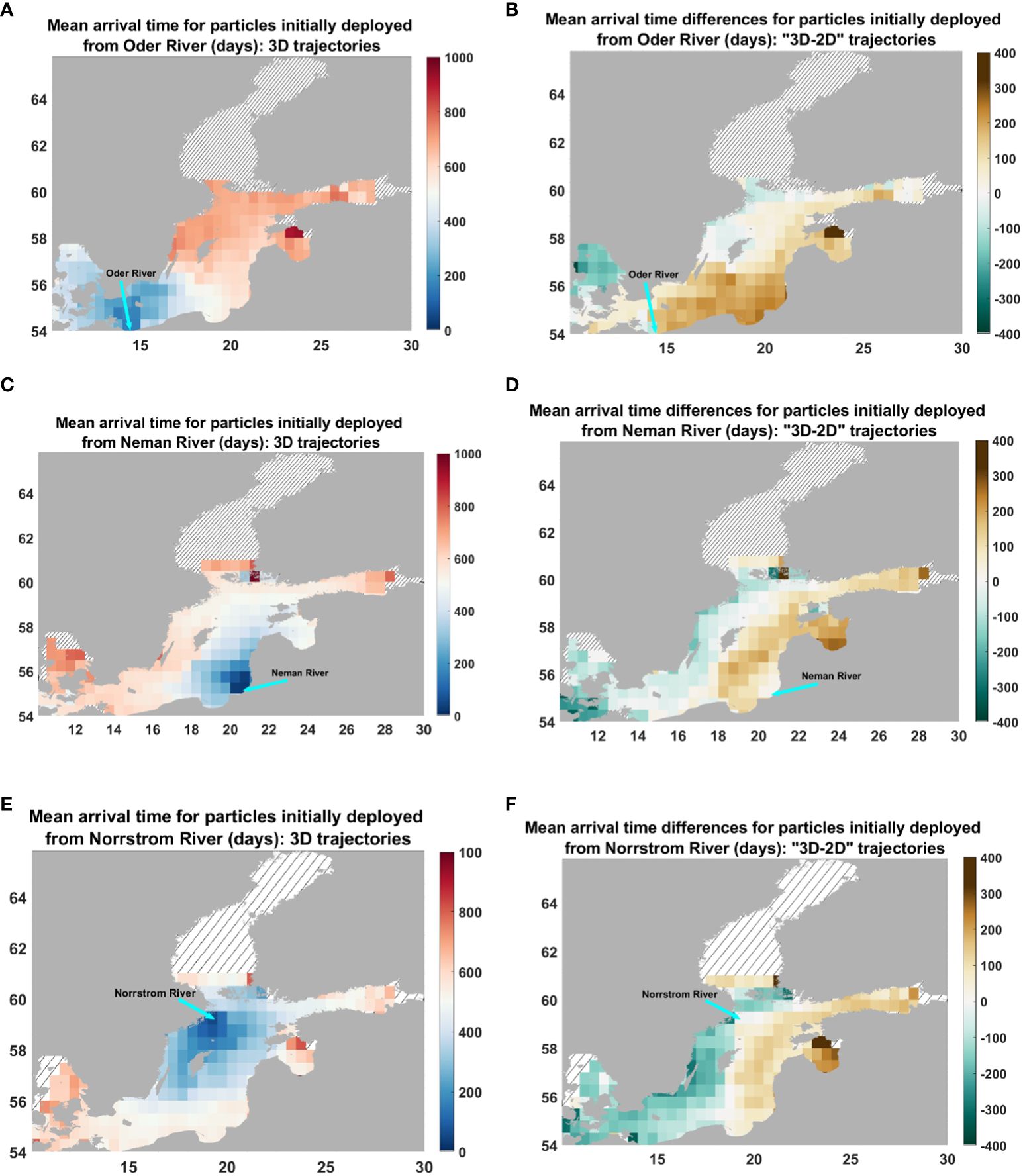
Figure 6 Mean transit times for 3D trajectories in HR3D-250m during 2011-2013 and the differences between 3D and 2D trajectories (HR3D-250m minus HR2D-250m): (A, B) particle initially deployed from Oder River; (C, D) particle initially deployed from Neman River; (E, F) particle initially deployed from Norrström River.

In the 3D simulation, particles initially deployed near the Norrström River predominantly follow the current on the western side of the basin (Figure 6). In contrast, particles in the 2D simulation move faster towards the eastern part of the Gotland Basin and into the GoF and GoR than towards south. The results in the 3D simulation seem to align with the observed pattern elucidated by Elken and Matthäus (2008) in their comprehensive circulation scheme. In HR3D-250m, particles need for their travel from the western side of the Gotland Basin into the GoF more than 600 days, while in HR2D-250m only 450 days are needed.

Furthermore, we compared the trajectories in 2D and 3D for particles initially released from the Neman River (Figure 6). The observed patterns were similar to those witnessed for particles initially released from the Oder River. The presence of downwelling in the eastern and southeastern regions of the basin has a significant impact on the behavior of numerical particles in 3D simulations. This results in longer transit times when compared to 2D simulations.

3.2.2 Mean arrival depth

To delve deeper into the effects of vertical advection, we calculated the average depth reached by particles initially released from various river mouths in the Baltic Sea. (Figure 7). This analysis aims to establish the connectivity between coastal regions and the open sea. Initially, we released particles from the surface layer to a maximum depth of 20 meters and tracked their trajectories to various areas of the basin. Our results indicate that particles released from the Norrström River typically arrive at a mean depth of 25 meters near the Gotland Basin. The deepest areas they reach are in the Gulf of Finland and the southeastern part of the basin, with a mean depth ranging from 50 to 65 meters. Comparing these results with mean transit time maps reveals that these regions also exhibit longer transit time values than the rest of the basin.

Figure 7

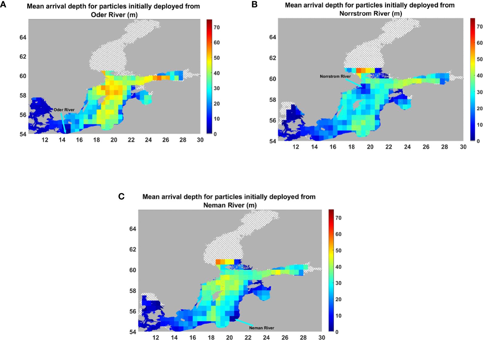
Figure 7 Mean arrival depth for 3D trajectories: (A) particle initially deployed from Oder River; (C, B) particle initially deployed from Norrström River; (C) particle initially deployed from Neman River.

Our analysis of particles released from other river mouths highlights that those from the Oder River or Neman River are influenced by vertical advection and move much deeper than those from the Norrström River (Figure 7). The results of Oder River particles indicate a mean arrival depth of over 45 meters for the central part of the Gotland Basin and adjacent areas such as the NGB and GoF. These particles follow the bottom topography of the Baltic Sea due to dense gravity currents, moving to the deeper parts of the basin around the northern Gotland and southwestern Swedish coast.

3.2.3 Network connections

For the network analysis, we focused on specific regions as destination sites and calculated the probability density function (PDF) of the Lagrangian parameters, including minimum arrival transit time and arrival depths, for numerical particles initially deployed from different river mouths (Figures 8, 9; Supplementary Figures S6, S7, S8, S9). Our approach enabled us to identify key findings on the exchange between coastal areas and the rest of the basin. We selected sites based on the topography of the Baltic Sea to compare the 2D and 3D connectivity properties of the basin (Figure 1). Sites A, C, D, and G were chosen due to their location in the deeper areas of the basin. Site B was selected specifically to investigate the behavior of particles in the southern part of WGB. Site F is associated with the Gdansk Basin. Sites E and H were chosen for their representation of the deeper areas in the Arkona Basin and the southern EGB, respectively.

Figure 8

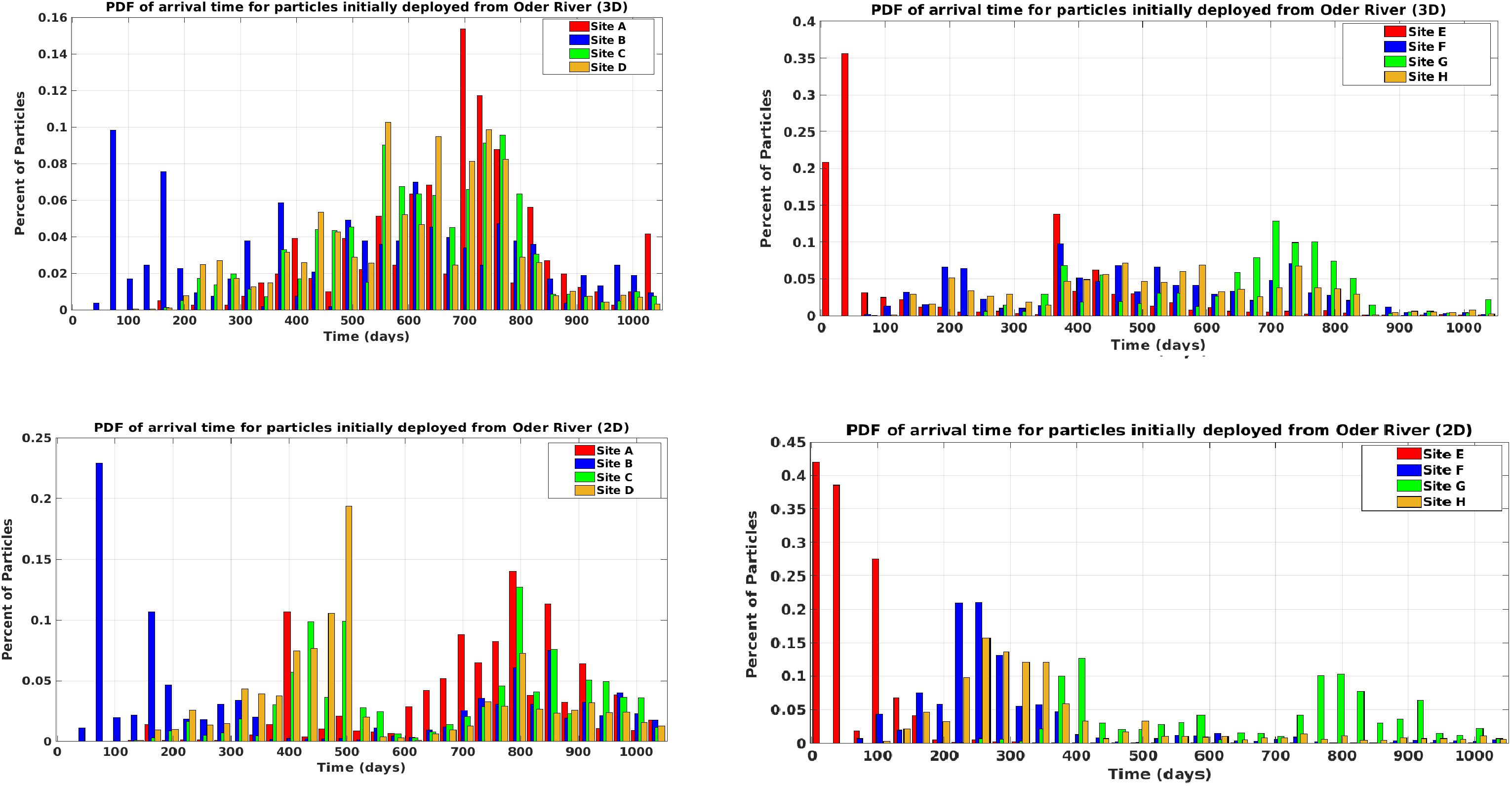
Figure 8 Comparison of PDF of arrival transit time (in all depths) to the destination sites for particles initially deployed from Oder River (2D vs. 3D trajectories).

Figure 9

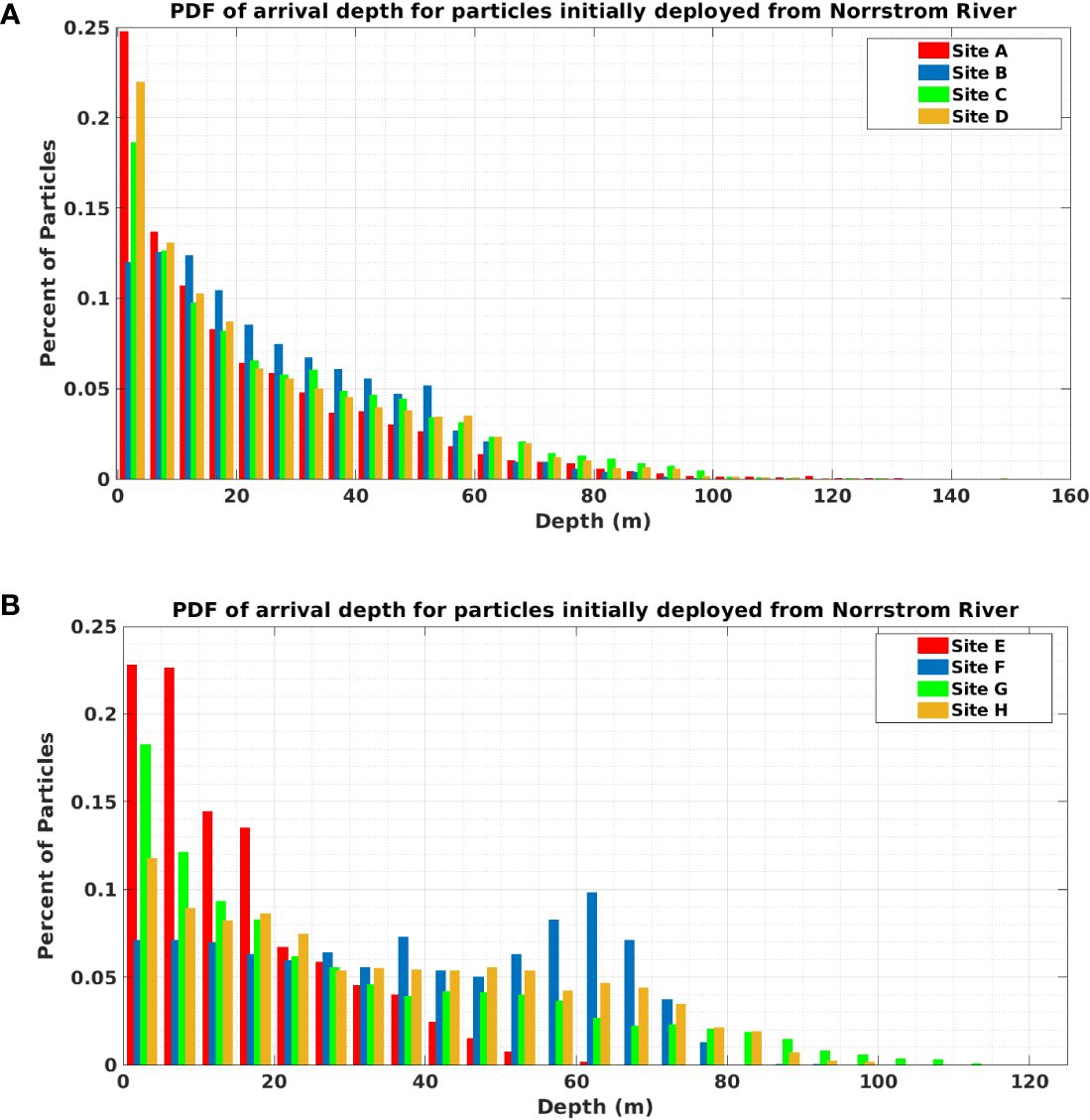
Figure 9 Comparison of PDF of arrival depth to the destination sites for particles initially deployed from Norrström River, (A) destination sites A,B, C and D; (B) destination sites E,F,G and H.

Figure 8 displays the PDFs of transit times for particles traveling from the Oder River to the selected sites in HR3D-250m and HR2D-250m. The PDFs are non-Gaussian and skewed, with a long tail. In HR2D-250m, over 18% of particles arrive at site A in less than a year, whereas in HR3D-250m this value is less than 10%. The same behavior is observed for site B, where a greater percentage of particles arrive in HR2D-250m compared to HR3D-250m over a shorter period (i.e., a difference of about 100 days). The peak values for HR3D-250m are between 700 to 750 days, while over 30% of particles take between 700 to 750 days to move from the Oder River to site A. Conversely, in HR2D-250m, one peak value is approximately 400 days, while the other is about 800 to 850 days (Figure 8).

For sites nearer to the initial particle position, such as site E, the transit time of numerical particles is shorter, and over 90% of particles arrive at site E in less than 100 days in HR2D-250m, but this value is less than 60% for HR3D-250m. Moreover, the effects of high-density inflow water on numerical particle movement are observable through changes in travel times.

When examining site D on the eastern side of the Gotland Basin, results from HR3D-250m indicate that the first particles arrive in about 200 days in HR3D-250m, whereas for HR2D-250m, the first particles arrive in less than 175 days. Furthermore, in HR3D-250m the peak values are distributed more widely between 550 and 750 days, but in HR2D-250m, the peak values of transit time are concentrated to less than 500 days.

We conducted an analysis of the transit time PDF distribution for particles arriving from the Oder River to the Gulf of Gdansk. The PDF width in HR3D-250m is wider compared to the HR2D-250m, which suggests that particles have a larger but slower spread across the domain before reaching the Gulf of Gdansk. As shown in Figure 8, the majority of particles arrive in the Gulf of Gdansk in less than 400 days in the 2D simulation, whereas in the 3D simulation the arrival time for particles is distributed from 100 days to more than 800 days.

The results for other rivers demonstrate that, owing to vertical advection, a larger number of particles reaches site A (located on the western side of the Gotland Basin) in less than a month compared to the 2D simulation. This pattern confirms our previous findings that in 2D particles on the north-west side of the Gotland Basin are more influenced by sub-mesoscale structures than in the 3D simulation (Supplementary Figures S6, S8). Furthermore, particles originating from the Norrström River reach site B near Öland island at a faster rate in 3D compared to 2D trajectories (Supplementary Figure S6).

In addition, our results reveal significant differences in the behavior of particles arriving at site F (Bay of Gdansk) from Norrström River between 2D and 3D simulations. In 3D, particles require between 100 to 800 days to reach the site, whereas in 2D, the range of transit time is broader, extending up to 1000 days. Nevertheless, the mean transit time for both cases is similar (Supplementary Figure S6).

We also examined the PDFs of arrival depth for various simulations, showing distinct patterns based on the initial position of the particles (Figure 9; Supplementary Figures S7, S9). When particles were deployed from the western side of the Baltic Sea (Norrström River), the majority arriving at sites A, B, C, D, E, and G remained at depths less than 120 meters (Figure 9). The PDF plots for these sites exhibited similar distributions, with a long tail indicating a decrease in the percentage of particles arriving as the depth increased. However, for sites F (Bay of Gdansk) and G (the northern Baltic Sea), the PDF plots show a different pattern, with a higher percentage of particles moving deeper (Figure 9).

3.3 Residence time

We released numerical particles from diverse locations (uniformly) across the Baltic Sea’s surface layer, allowing them to undergo integration for a maximum period of eight years using the HR2D-250m model. Subsequently, we calculated the residence time for particles exiting the Baltic Sea within the eight years (Figure 10). Our analysis reveals that, on average, numerical particles spend approximately 790 days within the Baltic Sea during this extended integration period of eight years.

Figure 10

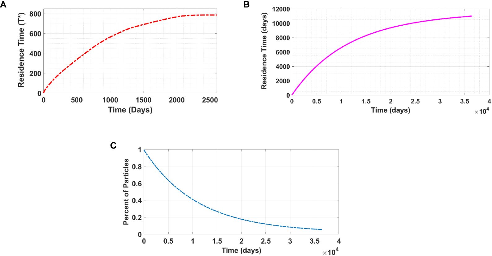
Figure 10 (A) Residence time (days) for only surface particles exiting the basin during 8 years; (B) residence time (days) for all particles exiting from the basin; (C) dissipation rate of numerical particles.

Moreover, when we considered the decay or dissipation rate of the numerical particles, we conducted an analysis to determine the ultimate lifetime of these particles within the Baltic Sea. It was established that it takes an estimated 95 years for the final particles to exit the basin. Additionally, the average residence time for numerical particles in the Baltic Sea, calculated through Equations 3–7 and focusing on all released particles amounts to approximately 29 years. This finding closely corresponds to the findings reported by Döös et al. (2004). Döös et al. (2004) estimated the residence time for the entire Baltic to be around 25-30 years, calculated as the ratio of volume to flow.

4 Discussion

Applying a Lagrangian approach proves effective in examining oceanic connectivity, but its utility is tempered by inherent limitations and challenges, prompting numerous scientific inquiries. A significant obstacle lies in the dependence on numerical models (OGCMs) and the assumption of their precise representation of intricate physical processes in basins like the Baltic Sea. While these models yield valuable insights, they fall short as perfect substitutes for direct observational data, as internal variability and uncertainties in model outputs may compromise result robustness.

Our study highlights the impact of model resolution on results. Higher resolutions offer finer details but come with increased computational demands. We often face a trade-off between computational feasibility and the need for higher resolution to capture the nuances of sub-mesoscale structures and eddies. This trade-off presents a challenge for modeling oceanic connectivity effectively.

The primary objective of our work was to explore ocean connectivity in the Baltic Sea due to the effects of sub-mesoscale features using Lagrangian numerical particles and the OceanParcels Lagrangian particle tracking model. Statistically robust estimates were derived from extensive particle deployments and three distinct simulations.

The findings, based on diverse Lagrangian indices, offer insights into the interconnectedness of different Baltic Sea regions, crucial for effective ecosystem management and conservation. Identifying key areas of exchange and influencing factors aids in guiding conservation efforts and marine spatial planning. Additionally, the revelation of slow circulation and pollutant accumulation underscores the urgency of addressing pollution’s impact on the ecosystem. Furthermore, upon comparing the results obtained from two distinct model resolutions (HR-250m and HR-1km), we identify significant differences in the connection transit time among various rivers (Figure 4). Our results also suggest a nuanced picture of the regional oceanic currents during the study period. It appears that, on average, the currents flowing from the southern regions of the Baltic Sea toward the eastern side possessed slightly greater strength when compared to currents originating from the northern side of the Gotland Basin, which were directed towards the western Baltic. Coastal upwelling and downwelling are significant factors, particularly along the western and eastern coastal zones of the Baltic Sea. These processes have a crucial impact on how particles move around. They can either speed up or slow down the transportation of particles, helping them to reach the upper layer of the sea basin more rapidly or slowly. These findings are significant in explaining and predicting the dispersion of various species in the Baltic Sea and their movements in the basin. Moreover, this underlines the sensitivity of particle behavior to the model resolution and the role of fine-scale structures in driving transport patterns. Scientifically, this highlights the need for more detailed models to capture these complex dynamics effectively.

The investigation into vertical advection and its influence on particle movement is a significant contribution to the understanding of Baltic Sea dynamics. The observation of extended transit times in the 3D simulation, particularly in the southern Baltic and the Baltic proper, suggests the importance of considering three-dimensional processes in connectivity analysis. This finding raises questions about the ecological consequences of longer transit times, as particles may transport nutrients and contaminants over larger distances. Future research in this area could explore the ecological implications further.

In general, the complex 3D flow pattern in the Baltic Sea is influenced by factors such as bathymetry and wind forcing, where the deep inflow and surface outflow converge and mix. However, the 2D flow is characterized by the influence of coastal currents, primarily a portion of the return flow from the northern Gotland Basin.

Furthermore, the shape of the PDF plots of transit times between selected sites shown in Figure 8 can be significantly affected by various factors, such as velocity fields, source and destination sites, and flow patterns. The complex and variable flow patterns can greatly influence the distribution of particles that arrive at the destination site. Moreover, when the current between two sites is fast and unidirectional, the resulting PDF tends to be narrow and peaked, indicating that particles arrive at the destination site quickly and with minimal variation in arrival time. Conversely, if the current is slower and more variable, the PDF may be wider and flatter, suggesting that particles arrive at the destination site over a broader time range and with more variation in arrival time. Furthermore, the presence of eddies or other flow features that cause particles to meander or change direction can also impact the PDF’s shape. Variations in source or destination locations can alter the path and travel time of particles, which can then influence the PDF. Therefore, the shape of the PDF can qualitatively change depending on the dynamical properties of the advection pattern in flows.

The calculation of the average residence time (29 years for all particles exiting from the basin) highlights the Baltic Sea’s slow circulation, contributing to the accumulation of pollutants and nutrients. This finding underscores the ecological relevance of understanding the dynamics of particle transport and mixing in the Baltic Sea. It connects scientific research to broader environmental concerns, particularly the issue of eutrophication, which has practical implications for the management of the Baltic Sea’s ecosystem.

Consequently, in coarse-resolution simulations, the dispersion of particles is compromised, leading to prolonged transit times and restricted connectivity between different areas. To address this issue when incorporating Lagrangian trajectories using velocities computed in coarse-resolution simulations, a potential solution involves parameterizing the absent dispersion. Various methods have been suggested in the literature, with the simplest involving the addition of a random walk to each particle’s successive position. This method aligns with an advection–diffusion equation and corresponds to a stochastic “Markovian” parameterization (Berloff and McWilliams, 2002). However, this stochastic approach falls short in replicating small-scale ocean dynamics that entail consistency in advection (Klocker et al., 2012a; Klocker et al., 2012b; Veneziani et al., 2004). In attempts to better capture the effects of small-scale ocean dynamics, higher-order Markov parameterizations have been proposed (Berloff and McWilliams, 2002; Griffa, 1996; Rodean, 1996; Sawford, 1991). Enhanced parameterizations also involve considerations such as particle looping due to eddy coherence (Reynolds, 2002; Veneziani et al., 2004) and relative dispersion between different particles (Piterbarg, 2002). While these methods were initially developed for horizontal flows, recent advancements include isopycnal Markov-0 (Spivakovskaya et al., 2007) or shear-dependent formulations (Le Sommer et al., 2011). A more recent development is the isoneutral Markov-1 formulation (Reijnders et al., 2022), which seems to better emulate the coherent behavior of 3D ocean dispersion at small scales. It would be intriguing in future studies to assess how such methods, applied within a Lagrangian framework, might enhance the outcomes obtained from coarse-resolution field simulations.

5 Conclusion

In conclusion, the research presented in this paper advances our understanding of the Baltic Sea’s complex dynamics, particularly in terms of particle movement, transport patterns, and connectivity. Our study provides valuable insights into the connectivity of particles originating from selected river mouths across different coastal sections of the Baltic Sea.

i. Our analysis reveals varying connectivity strengths among these particles due to sub-mesoscale structures. These fine-scale structures play a pivotal role in shaping connections between different coastal sections. The differences in connectivity, assessed through particle analysis, showcase average differences of up to 27% between simulations with and without sub-mesoscale structures.

ii. Furthermore, our investigation delves into the contrasting trajectories of freshwater particles in 2D versus 3D simulations. The outcomes emphasize that 3D particle movements differ significantly from their 2D simulations, underscoring the critical role of vertical currents in understanding particle dynamics.

iii. Within the Baltic Sea, we’ve observed travel times for particles from the coastal zone to interior sub-basins with sub-mesoscale structures ranging between 350 and 1650 days, depending on the initial position of the particles. Without sub-mesoscale structures travel times extend approximately from 500 to 1900 days.

iv. Our findings strongly indicate that fine-scale structures notably contribute to particle dispersal. The calculated average residence time for all freshwater particles exiting the Baltic Sea is approximately 29 years, while the lifetime extends to about 95 years for the last particles to exit the basin.

In summary, our study has unraveled the intricate dynamics of particle connectivity, highlighting the crucial roles of sub-mesoscale structures, 2D and 3D trajectories, and residence times in shaping the environmental and ecological dynamics of the Baltic Sea. However, capturing the full spectrum of 3D oceanic dynamics remains a substantial challenge, particularly in regions characterized by complex bathymetry.

Data availability statement

The datasets presented in this article are not readily available because major parts of the data and codes used in this study are available upon request by contacting the corresponding author at saeed.hariri@io-warnemuende.de. Please note that access to the codes may be subject to restrictions due to privacy or confidentiality concerns. Requests to access the datasets should be directed to saeed.hariri@io-warnemuende.de.

Author contributions

SH: Conceptualization, Data curation, Formal analysis, Funding acquisition, Investigation, Methodology, Resources, Software, Validation, Visualization, Writing – original draft, Writing – review & editing. HEMM: Conceptualization, Funding acquisition, Methodology, Resources, Supervision, Validation, Visualization, Writing – review & editing. GV: Data curation, Formal analysis, Investigation, Methodology, Visualization, Writing – review & editing.

Funding

The author(s) declare financial support was received for the research, authorship, and/or publication of this article. The study is a contribution to the BMBF funded project CoastalFutures (03F0911E) which supported SH. GV was supported by the Estonian Research Council (grant PRG602) and Leibniz Institute for Baltic Sea research (IOW) during the visits to Warnemünde.

Acknowledgments

The presented research is part of the Baltic Earth programme (Earth System Science for the Baltic Sea region, see http://baltic.earth) and the new focus programme on “Shallow Water Processes and Transitions to the Baltic Scale” at the Leibniz Institute of Baltic Sea Research Warnemünde (https://www.io-warnemuende.de/stb-shallow-water-processes.html). Computational resources from HLRN (project mvk00075) and HPC of Tallinn University of Technology are gratefully acknowledged. The GETM community at Leibniz Institute of Baltic Sea Research is acknowledged for maintaining and supporting the model code.

Conflict of interest

The authors declare that the research was conducted in the absence of any commercial or financial relationships that could be construed as a potential conflict of interest.

Publisher’s note

All claims expressed in this article are solely those of the authors and do not necessarily represent those of their affiliated organizations, or those of the publisher, the editors and the reviewers. Any product that may be evaluated in this article, or claim that may be made by its manufacturer, is not guaranteed or endorsed by the publisher.

Supplementary material

The Supplementary Material for this article can be found online at: https://www.frontiersin.org/articles/10.3389/fmars.2024.1340291/full#supplementary-material

References

Alberto F., Raimondi P. T., Reed D. C., Watson J. R., Siegel D. A., Mitarai S., et al. (2011). Isolation by oceanographic distance explains genetic structure for Macrocystis pyrifera in the Santa Barbara Channel. Mol. Ecol. 20, 2543–2554. doi: 10.1111/j.1365-294X.2011.05117.x

PubMed Abstract | CrossRef Full Text | Google Scholar

Berloff P. S., McWilliams J. C. (2002). Material transport in oceanic gyres, part II: Hierarchy of stochastic models. J. Phys. Oceanogr. 32, 797–830. doi: 10.1175/1520-0485(2002)0322.0.co;2

CrossRef Full Text | Google Scholar

Bharti D. K., Katell Guizien M. T., Aswathi-Das P. N., Vinayachandran K. S. (2022). Connectivity networks and delineation of disconnected coastal provinces along the Indian coastline using large-scale Lagrangian transport simulations. Limnology Oceanography 67, 1416–1428. doi: 10.1002/lno.12092

CrossRef Full Text | Google Scholar

Blanke B., Raynaud S. (1997). Kinematics of the Pacific Equatorial Undercurrent: An Eulerian and Lagrangian approach from GCM results. J. Phys. Oceanography 27, 1038–1053. doi: 10.1175/1520-0485(1997)027%3C1038:KOTPEU%3E2.0.CO;2

CrossRef Full Text | Google Scholar

Buffoni G., Falco P., Griffa A., Zambianchi E. (1997). Dispersion processes and residence times in a semi-enclosed basin with recirculating gyres: An application to the Tyrrhenian Sea. J. Geophys. Res. 102, 18699–18713. doi: 10.1029/96JC03862

CrossRef Full Text | Google Scholar

Burchard H., Bolding K. (2001). Comparative analysis of four second-moment turbulence closure models for the oceanic mixed layer. J. Phys. Oceanogr. 31, 1943–1968. doi: 10.1175/1520-0485(2001)031<1943:CAOFSM>2.0.CO;2

CrossRef Full Text | Google Scholar

Burchard H., Bolding Kristensen K. (2002). GETM, a General Estuarine Transport Model (EUR 20253 EN. European Commission; 2002. JRC23237). Available online at: https://publications.jrc.ec.europa.eu/repository/handle/JRC23237 (Accessed 26.02.2024).

Google Scholar

Canuto V. M., Howard A., Cheng Y., Dubovikov. M. S. (2001). Ocean turbulence. Part I: One-point closure model-momentum and heat vertical diffusivities. J. Phys. Oceanogr. 31, 1413–1426. doi: 10.1175/1520-0485(2001)031<1413:OTPIOP>2.0.CO;2

CrossRef Full Text | Google Scholar

Christensen A., Murawski J., She J., St. John M. (2023). Simulating transport and distribution of marine macro-plastic in the Baltic Sea. PloS One 18, e0280644. doi: 10.1371/journal.pone.0280644

PubMed Abstract | CrossRef Full Text | Google Scholar

Chrysagi E., Umlauf L., Holtermann P., Klingbeil K., Burchard H. (2021). High-resolution simulations of submesoscale processes in the Baltic Sea: The role of storm events. J. Geophysical Research: Oceans 126, e2020JC016411. doi: 10.1029/2020JC016411

CrossRef Full Text | Google Scholar

Corell H., Döös K. (2013). Difference in particle transport between two coastal areas in the baltic sea investigated with high-resolution trajectory modeling. AMBIO 42, 455–463. doi: 10.1007/s13280-013-0397-3

PubMed Abstract | CrossRef Full Text | Google Scholar

Corell H., Moksnes P. O., Engqvist A., Döös K., Jonsson. P. R. (2012). Depth distribution of larvae critically affects their dispersal and the efficiency of marine protected areas. Mar. Ecol. Prog. Ser. 467, 29–46. doi: 10.3354/meps09963

CrossRef Full Text | Google Scholar

Cristiani J., Rubidge E., Forbes C., Moore-Maley B., O’Connor M. I. (2021). A biophysical model and network analysis of invertebrate community dispersal reveals regional patterns of seagrass habitat connectivity. Front. Mar. Sci. 8. doi: 10.3389/fmars.2021.717469

CrossRef Full Text | Google Scholar

Dargahi B. (2022). Lagrangian coherent structures and hypoxia in the baltic sea. Dynamics Atmospheres Oceans 97, 101286. doi: 10.1016/j.dynatmoce.2022.101286

CrossRef Full Text | Google Scholar

Dever E. P., Hendershott M. C., Winant. C. D. (1998). Statistical aspects of surface drifter observations of circulation in the Santa Barbara Channe. J. Geophys. Res. Oceans 103, 24781–24797. doi: 10.1029/98JC02403

CrossRef Full Text | Google Scholar

Dong C., Idica E. Y., McWilliams J. C. (2009). Circulation and multi-scale variability in the southern california bight. Prog. Oceanography 82, 168–190. doi: 10.1016/j.pocean.2009.07.005

CrossRef Full Text | Google Scholar

Dong C., McWilliams J. C. (2007). A numerical study of island wakes in the Southern California Bight. Continental Shelf Res. 27, 1233–1248. doi: 10.1016/j.csr.2007.01.016

CrossRef Full Text | Google Scholar

Döös K., Meier H. E. M., Döscher R. (2004). The baltic haline conveyor belt or the overturning circulation and mixing in the baltic. AMBIO: A J. Hum. Environ. 33, 261–266. doi: 10.1579/0044-7447-33.4.261

CrossRef Full Text | Google Scholar

Drouet K., Jauzein C., Herviot-Heath D., Hariri S., Laza-Martinez A., Lecadet C., et al. (2021). Current Distribution and Potential Expansion of the Harmful Benthic Dinoflagellate Ostreopsis cf. siamensis towards the Warming Waters of the Bay of Biscay, North-East Atlantic. Environ. Microbiol. 23, 4956–4979. doi: 10.1111/1462-2920.15406

PubMed Abstract | CrossRef Full Text | Google Scholar

Elken J., Matthäus W. (2008). “Physical system description,” in Assessment of Climate Change for the Baltic Sea Basin. Series: Regional climate studies. Ed. von Storch ,. H. (Springer-Verlag, Berlin, Heidelberg), 379–398.

Google Scholar

Emelyanov E. M. (1995). Baltic sea: geology, geochemistry, paleoceanography, pollution. P.P. Shirshov institute of oceanology RAS, atlantic branch baltic ecological institute of hydrosphere academy of natural sciences. (Moscow: Shirshov Institute of Oceanology, The Russian Academy of Sciences), 115.

Google Scholar

Giudici A., Suara K. A., Soomere T., Brown R. (2021). Tracking areas with increased likelihood of surface particle aggregation in the gulf of Finland: A first look at persistent lagrangian coherent structures (LCS). J. Mar. Syst. 217, 103514. doi: 10.1016/j.jmarsys.2021.103514

CrossRef Full Text | Google Scholar

Griffa A. (1996). “Applications of stochastic particle models to oceanographic problems,” in Stochastic modelling in physical oceanography. Eds. Adler R. J., Müller P., Rozovskii B. L. (Birkhäuser Boston), 113–140. doi: 10.1007/978-1-4612-2430-3_5

CrossRef Full Text | Google Scholar

Gräwe U., Holtermann P., Klingbeil K., Burchard H. (2015). Advantages of vertically adaptive coordinates in numerical models of stratified shelf seas. Ocean Model. 92, 56–68. doi: 10.1016/j.ocemod.2015.05.008

CrossRef Full Text | Google Scholar

Gräwe U., Klingbeil K., Kelln J., Dangendorf S. (2019). Decomposing mean sea level rise in a semi-enclosed basin, the baltic sea. J. Climate 32, 3089–3108. doi: 10.1175/JCLI-D-18-0174.1

CrossRef Full Text | Google Scholar

Gröger M., Placke M., Meier H. E. M., Börgel F., Brunnabend S.-E., Dutheil C., et al. (2022). The baltic sea model intercomparison project (BMIP) – A platform for model development, evaluation, and uncertainty assessment. GMD 15, 8613–8638. doi: 10.5194/gmd-15-8613-2022

CrossRef Full Text | Google Scholar

Hariri S. (2020). Near-surface transport properties and lagrangian statistics during two contrasting years in the adriatic sea. J. Mar. Sci. Eng. 8, 681. doi: 10.3390/jmse8090681

CrossRef Full Text | Google Scholar

Hariri S. (2022). Analysis of mixing structures in the adriatic sea using finite-size lyapunov exponents. Geophysical Astrophysical Fluid Dynamics 116, 20–37. doi: 10.1080/03091929.2021.1962851

CrossRef Full Text | Google Scholar

Hariri S., Besio G., Stocchino A. (2015). Comparison of Finite Time Lyapunov Exponent and Mean Flow Energy During Two Contrasting Years in the Adriatic Sea, OCEANS’15 MTS/IEEE, Genoa, Italy. doi: 10.1109/OCEANS-Genova.2015.7271418

CrossRef Full Text | Google Scholar

Hariri S., Plus M., Le Gac M., Séchet V., Revilla M., Sourisseau M. (2022). Advection and composition of dinophysis spp. Populations along the european atlantic shelf. Front. Mar. Sci. 9. doi: 10.3389/fmars.2022.914909

PubMed Abstract | CrossRef Full Text | Google Scholar

Hofmeister R., Burchard H., Beckers J.-M. (2010). Non-uniform adaptive vertical grids for 3D numerical ocean models. Ocean Model. 33, 70–86. doi: 10.1016/j.ocemod.2009.12.003

CrossRef Full Text | Google Scholar

Jonsson P. R., Moksnes P.-O., Corell H., Bonsdorff E., Nilsson Jacobi M. (2020). Ecological coherence of marine protected areas: new tools applied to the baltic sea network. Aquat. Conservation: Mar. Freshw. Ecosyst. 30, 743–760. doi: 10.1002/aqc.3286

CrossRef Full Text | Google Scholar

Jönsson B., Watson J. (2016). The timescales of global surface-ocean connectivity. Nat. Commun. 7, 11239. doi: 10.1038/ncomms1123

PubMed Abstract | CrossRef Full Text | Google Scholar

Kinlan B. P., Gaines S. D. (2003). Propagule dispersal in marine and terrestrial environments: A community perspective. Ecology 84, 2007–2020. doi: 10.1890/01-0622

CrossRef Full Text | Google Scholar

Kjellsson J., Döös K. (2012). Lagrangian decomposition of the hadley and ferrel cells. Geophysical Res. Lett. 39. doi: 10.1029/2012GL052420

CrossRef Full Text | Google Scholar

Kjellsson J., Döös K., Soomere T. (2013). Evaluation and Tuning of Model Trajectories and Spreading Rates in the Baltic Sea Using Surface 35 Drifter Observations (Heidelberg: Springer International Publishing), 251–281. doi: 10.1007/978-3-319-00440-2_8

CrossRef Full Text | Google Scholar

Klingbeil K., Lemarié F., Debreu L., Burchard H. (2018). The numerics of hydrostatic structured-grid coastal ocean models: state of the art and future perspectives. Ocean Model. 125, 80–105. doi: 10.1016/j.ocemod.2018.01.007

CrossRef Full Text | Google Scholar

Klocker A., Ferrari R., LaCasce J. H. (2012a). Estimating suppression of eddy mixing by mean flows. J. Phys. Oceanogr. 42, 1566–1576. doi: 10.1175/JPO-D-11-0205.1

CrossRef Full Text | Google Scholar

Klocker A., Ferrari R., Lacasce J. H., Merrifield S. T. (2012b). Reconciling float-based and tracer-based estimates of lateral diffusivities. J. Mar. Res. 70, 569–602. doi: 10.1357/002224012805262743

CrossRef Full Text | Google Scholar

Krauss W., Brügge B. (1991). Wind-produced water exchange between the deep basins of the baltic sea. J. Phys. Oceanography 21, 373–384. doi: 10.1175/1520-0485(1991)021%3C0373:WPWEBT%3E2.0.CO;2

CrossRef Full Text | Google Scholar

LaCasce J. H. (2008). Statistics from lagrangian observations. Prog. Oceanography 77, 1–29. doi: 10.1016/j.pocean.2008.02.002

CrossRef Full Text | Google Scholar

Lange M., van Sebille E. (2017). Parcels v0.9: prototyping a lagrangian ocean analysis framework for the petascale age. Geoscientific Model. Dev. 10, 4175–4186. doi: 10.5194/gmd-10-4175-2017

CrossRef Full Text | Google Scholar

Largier J. L. (2003). Considerations in estimating larval dispersal distances from oceanographic data. Ecol. Appl. 13, S71–S89. doi: 10.1890/1051-0761(2003)013[0071:CIELDD]2.0.CO;2

CrossRef Full Text | Google Scholar

Lass H. U., Matthäus W. (2008). “General Oceanography of the Baltic Sea,” in State and Evolution of the Baltic Sea 1952-2005: A Detailed 50-Year Survey of Meteorology and Climate, Physics, Chemistry, Biology, and Marine Environment. Ed. Feistel R., Nausch G., Wasmund N.. (Hoboken, New Jersey: John Wiley & Sons, Inc).

Google Scholar

Lehmann A., Myrberg K. (2008). Upwelling in the baltic sea – A review. J. Mar. Syst. 74, S3–S12. doi: 10.1016/j.jmarsys.2008.02.010

CrossRef Full Text | Google Scholar

Lehmann A., Myrberg K., Post P., Chubarenko I., Dailidiene I., Hinrichsen H.-H., et al. (2022). Salinity dynamics of the baltic sea. Earth System Dynamics 13, 373. doi: 10.5194/esd-13-373-2022

CrossRef Full Text | Google Scholar

Leppäranta M., Myrberg K. (2009). Physical oceanography of the Baltic Sea (Berlin: Springer).

Google Scholar

Le Sommer J., d’Ovidio F., Madec G. (2011). Parameterization of subgrid stirring in eddy resolving ocean models, part 1: Theory and diagnostics. Ocean Model. 39, 154–169. doi: 10.1016/j.ocemod.2011.03.007

CrossRef Full Text | Google Scholar

Liblik T., Väli G., Lips I., Lilover M.-J., Kikas V., Laanemets J. (2020). The winter stratification phenomenon and its consequences in the Gulf of Finland, Baltic Sea. Ocean Sci. 16, 1475–1490. doi: 10.5194/os-16-1475-2020

CrossRef Full Text | Google Scholar

Liblik T., Väli G., Salm K., Lips U., Laanemets J., Lilove M.-J. (2022). ADCP and GETM simulation data in the Baltic Proper. Zenodo. doi: 10.5281/zenodo.6616795

CrossRef Full Text | Google Scholar

Lindström G., Pers C., Rosberg J., Strömqvist J., Arheimer B. (2010). Development and testing of the HYPE (Hydrological Predictions for the Environment) water quality model for different spatial scales. Hydrol. Res. 41, 295–319. doi: 10.2166/nh.2010.007

CrossRef Full Text | Google Scholar

Lips U., Kikas V., Liblik T., Lips I. (2016). Multi-sensor in situ observations to resolve the sub-mesoscale features in the stratified Gulf of Finland, Baltic Sea. Ocean Sci. 12, 715–732. doi: 10.5194/os-12-715-2016

CrossRef Full Text | Google Scholar

McWilliams J. C. (2016). Submesoscale currents in the ocean. Proc. Math. Phys. Eng. Sci. 472 (2189), 20160117. doi: 10.1098/rspa.2016.0117

PubMed Abstract | CrossRef Full Text | Google Scholar

Meier H. E. M. (2007). Modeling the pathways and ages of inflowing salt-and freshwater in the Baltic Sea. Estuar. Coast. Shelf Sci. 74, 610–627. doi: 10.1016/j.ecss.2007.05.019

CrossRef Full Text | Google Scholar

Mitarai S., Siegel D. A., Watson J. R., Dong C., McWilliams J. C. (2009). Quantifying connectivity in the coastal ocean with application to the Southern California Bight. J. Geophysical Res. 114, C10026. doi: 10.1029/2008JC005166

CrossRef Full Text | Google Scholar

Mohrholz V. (2018). Major baltic inflow statistics – revised. Front. Mar. Sci. 5. doi: 10.3389/fmars.2018.00384

CrossRef Full Text | Google Scholar

Mora C., Treml E. A., Roberts J., Crosby K., Roy D., Tittensor D. P. (2012). High connectivity among habitats precludes the relationship between dispersal and range size in tropical reef fishes. Ecography 35, 89–96. doi: 10.1111/j.1600-0587.2011.06874.x

CrossRef Full Text | Google Scholar

Myrberg K., Andrejev O. (2003). Main upwelling regions in the Baltic Sea: a statistical analysis based on three-dimensional modelling. Boreal Env. Res. 8, 97–112.

Google Scholar

Omstedt A., Elken J., Lehmann A., Lepparanta M., Meier H. E. M., Myrberg K., et al. (2014). Progress in physical oceanography of the Baltic Sea during the 2003-2014 period. Prog. Oceanography 128, 139–171. doi: 10.1016/j.pocean.2014.08.010

CrossRef Full Text | Google Scholar

Onken R., Baschek B., Angel-Benavides I. M. (2020). Very high-resolution modelling of submesoscale turbulent patterns and processes in the Baltic Sea. Ocean Sci. 16, 657–684. doi: 10.5194/os-16-657-2020

CrossRef Full Text | Google Scholar

Piterbarg L. I. (2002). The top Lyapunov exponent for a stochastic flow modeling the upper ocean turbulence. SIAM J. Appl. Mathemat. 62, 777–800. doi: 10.1137/S0036139999366401

CrossRef Full Text | Google Scholar

Pope S. (1994). Lagrangian PDF methods for turbulent flows. Annu. Rev. Fluid Mechanics 26, 23–63. doi: 10.1146/annurev.fl.26.010194.000323

CrossRef Full Text | Google Scholar

Poulain P.-M., Hariri S. (2013). Transit and residence times in the Adriatic Sea surface as derived from drifter data and Lagrangian numerical simulations. Ocean Sci. 9, 713–720. doi: 10.5194/os-9-713-2013

CrossRef Full Text | Google Scholar

Poulain P.-M., Niiler P. (1989). Statistical analysis of the surface circulation in the California Current System using satellite-tracked drifters. J. Phys. Oceanography 19, 1588–1603. doi: 10.1175/1520-0485(1989)019<1588:SAOTSC>2.0.CO;2

CrossRef Full Text | Google Scholar

Radtke H., Brunnabend S.-E., Gräwe U., Meier H. E. M. (2020). Investigating interdecadal salinity changes in the Baltic Sea in a 1850–2008 hindcast simulation. Clim. Past 16, 1617–1642. doi: 10.5194/cp-16-1617-2020

CrossRef Full Text | Google Scholar

Reijnders D., Deleersnijder E., van Sebille E. (2022). Simulating lagrangian subgrid-scale dispersion on neutral surfaces in the ocean. J. Adv. Model. Earth Syst. 14, e2021MS002850. doi: 10.1029/2021MS002850

PubMed Abstract | CrossRef Full Text | Google Scholar

Reissmann J. H., Burchard H., Feistel R., Hagen E., Lass H. U., Mohrholz V., et al. (2009). Vertical mixing in the Baltic Sea and consequences for eutrophication – A review. Prog. Oceanography 82, 47–80. doi: 10.1016/j.pocean.2007.10.004

CrossRef Full Text | Google Scholar

Reynolds A. (2002). On lagrangian stochastic modelling of material transport in oceanic gyres. Physica D 172, 124–138. doi: 10.1016/S0167-2789(02)00660-7

CrossRef Full Text | Google Scholar

Rodean H. C. (1996). Stochastic lagrangian models of turbulent diffusion (Boston, MA: American Meteorological Society), 84. doi: 10.1007/978-1-935704-11-9

CrossRef Full Text | Google Scholar

Roiha P., Siiriä S.-M., Haavisto N., Alenius P., Westerlund A., Purokoski T. (2018). Estimating currents from argo trajectories in the bothnian sea, baltic sea. Front. Mar. Sci. 5. doi: 10.3389/fmars.2018.00308

CrossRef Full Text | Google Scholar

Roughgarden J., Gaines S., Possingham H. (1988). Recruitment dynamics in complex life-cycles. Science 241, 1460–1466. doi: 10.1126/science.11538249

PubMed Abstract | CrossRef Full Text | Google Scholar

Salm K., Liblik T., Lips U. (2023). Submesoscale variability in a mesoscale front captured by a glider mission in the Gulf of Finland, Baltic Sea. Front. Mar. Sci. 10. doi: 10.3389/fmars.2023.984246

CrossRef Full Text | Google Scholar

Sawford B. L. (1991). Reynolds number effects in lagrangian stochastic models of turbulent dispersion. Phys. Fluid. A 3, 1577–1586. doi: 10.1063/1.857937

CrossRef Full Text | Google Scholar

Ser-Giacomi E., Legrand T., Hernandez-Carrasco I., Rossi V. (2021). Explicit and implicit network connectivity: Analytical formulation and application to transport processes. Phys. Rev. E 103, 42309. doi: 10.1103/physreve.103.042309

CrossRef Full Text | Google Scholar

Siegel D., Kinlan B., Gaylord B., Gaines S. (2003). Lagrangian descriptions of marine larval dispersion. Mar. Ecol. Prog. Ser. 260, 83–96. doi: 10.3354/meps260083

CrossRef Full Text | Google Scholar

Sjöqvist C., Godhe A., Jonsson P. R., Sundqvist L., Kremp A. (2015). Local adaptation and oceanographic connectivity patterns explain genetic differentiation of a marine diatom across the North Sea-Baltic Sea salinity gradient. Mol. Ecol. 24, 2871–2885. doi: 10.1111/mec.13208

PubMed Abstract | CrossRef Full Text | Google Scholar

Smagorinsky J. (1963). General circulation experiments with the primitive equations. Mon. Wea. Rev. 91, 99–164. doi: 10.1175/1520-0493(1963)091<0099:GCEWTP>2.3.CO;2

CrossRef Full Text | Google Scholar

Soomere T., Döös K., Lehmann A., Meier H. E., Murawski J., Myrberg K., et al. (2014). The potential of current- and wind-driven transport for environmental management of the Baltic Sea. AMBIO 43 (1), 94–104. doi: 10.1007/s13280-013-0486-3

PubMed Abstract | CrossRef Full Text | Google Scholar

Spivakovskaya D., Heemink A. W., Deleersnijder E. (2007). Lagrangian modelling of multidimensional advection-diffusion with space-varying diffusivities: Theory and idealized test cases. Ocean Dynam. 57, 189–203. doi: 10.1007/s10236-007-0102-9

CrossRef Full Text | Google Scholar

Stramska M., Kowalewska-Kalkowska H., Świrgoń M. (2013). Seasonal variability in the Baltic Sea level. Oceanologia 55, 787–807. doi: 10.5697/oc.55-4.787

CrossRef Full Text | Google Scholar

Swenson M., Niiler P. (1996). Statistical analysis of the surface circulation of the California Current. J. Geophys. Res. 101, 22631–22645. doi: 10.1029/96JC02008

CrossRef Full Text | Google Scholar

Teacher A. G. F., André C., Jonsson P. R., Merilä J. (2013). Oceanographic connectivity and environmental correlates of genetic structuring in Atlantic herring in the Baltic Sea. Evolutionary Appl. 6, 549–567. doi: 10.1111/eva.12042

CrossRef Full Text | Google Scholar

Thomas L. N., Tandon A., Mahadevan A. (2008). Submesoscale processes and dynamics. Ocean modeling an Eddying Regime 177, 17–38. doi: 10.1029/177GM04

CrossRef Full Text | Google Scholar

Uurasjärvi E., Pääkkönen M., Setälä O., Koistinen A., Lehtiniemi M. (2021). Microplastics accumulate to thin layers in the stratified Baltic Sea. Environ. pollut. 268, 115700. doi: 10.1016/j.envpol.2020.115700

PubMed Abstract | CrossRef Full Text | Google Scholar

Väli G., Meier H. E. M., Liblik T., Radtke H., Klingbeil K., Gräwe U., et al. (2023). Submesoscale processes in the surface layer of the central Baltic Sea: a high resolution modelling study. Oceanologia. in press. doi: 10.1016/j.oceano.2023.11.002

CrossRef Full Text | Google Scholar

Väli G., Meier H. E. M., Placke M., Dieterich C. (2019). River runoff forcing for ocean modeling within the Baltic Sea Model Intercomparison Project, Meereswiss. Ber. Warnemünde 113, 1–25. doi: 10.12754/msr-2019-0113

CrossRef Full Text | Google Scholar

Väli G., Zhurbas V., Lips U., Laanemets J. (2017). Submesoscale structures related to upwelling events in the Gulf of Finland, Baltic Sea (numerical experiments). J. Mar. Syst. 171, 31–42. doi: 10.1016/j.jmarsys.2016.06.010

CrossRef Full Text | Google Scholar

Van Sebille E., England E. H., Froyland G. (2012). Origin, dynamics and evolution of ocean garbage patches from observed surface drifters. Environ. Res. Lett. 7, 44040. doi: 10.1088/1748-9326/7/4/044040

CrossRef Full Text | Google Scholar

Van Sebille E., Griffies S. M., Abernathey R., Adams T. P., Berloff P., Biastoch A., et al. (2018). Lagrangian ocean analysis: fundamentals and practices. Ocean Model. 121, 49–75. doi: 10.1016/j.ocemod.2017.11.008

CrossRef Full Text | Google Scholar

Veneziani M., Griffa A., Reynolds A. M., Mariano A. J. (2004). Oceanic turbulence and stochastic models from subsurface lagrangian data for the northwest atlantic ocean. J. Phys. Oceanogr. 34, 1884–1906. doi: 10.1175/1520-0485(2004)0342.0.co;2

CrossRef Full Text | Google Scholar

Vortmeyer-Kley R., Gräwe U., Feudel U. (2016). Detecting and tracking eddies in oceanic flow fields: a Lagrangian descriptor based on the modulus of vorticity. Nonlinear Processes Geophysics 23, 159–173. doi: 10.5194/npg-23-159-2016

CrossRef Full Text | Google Scholar

Wang Y., Raitsos D. E., Krokos G., Gittings J. A., Zhan P., Hoteit I. (2019). Physical connectivity simulations reveal dynamic linkages between coral reefs in the southern Red Sea and the Indian Ocean. Sci. Rep. 9, 16598. doi: 10.1038/s41598-019-53126-0

PubMed Abstract | CrossRef Full Text | Google Scholar

Watson J. R., Hays C. G., Raimondi P. T., Mitarai S., Dong C., McWilliams J. C., et al. (2011). Currents connecting communities: nearshore community similarity and ocean circulation. Ecology 92, 1193–1200. doi: 10.1890/10-1436.1

PubMed Abstract | CrossRef Full Text | Google Scholar

Winsor P., Rodhe J., Omstedt A. (2001). An analysis of 100 years of hydrographic data with a focus on the freshwater budget. Dim. Res. 18, 5–15. doi: 10.3354/cr018005

CrossRef Full Text | Google Scholar

Yi P., Chen X., Aldahan A., Possnert G., Hou X., Yu Z., et al. (2013). Circulation of water masses in the Baltic Proper revealed through iodine isotopes. Appl. Geochemistry 36, 118–124. doi: 10.1016/j.apgeochem.2013.05.014

CrossRef Full Text | Google Scholar

Zhurbas V., Väli G., Golenko M., Paka V. (2018). Variability of bottom friction velocity along the inflow water pathway in the Baltic Sea. J. Mar. Syst. 184, 50–58. doi: 10.1016/j.jmarsys.2018.04.008

CrossRef Full Text | Google Scholar

Zhurbas V., Väli G., Kuzmina N. (2019). Rotation of floating particles in submesoscale cyclonic and anticyclonic eddies: a model study for the southeastern Baltic Sea. Ocean Sci. 15, 1691–1705. doi: 10.5194/os-15-1691-2019

CrossRef Full Text | Google Scholar