 Jack D. Hollister1,2,3*Xiaohao Cai1Tammy Horton2,3Benjamin W. Price3Karolina M. Zarzyczny1,3Phillip B. Fenberg1,3
- 1School of Ocean and Earth Sciences, University of Southampton, Southampton, United Kingdom
- 2Ocean BioGeosciences, National Oceanography Centre, Southampton, United Kingdom
- 3Natural History Museum, London, United Kingdom
The shell morphology of limpets can be cryptic and highly variable, within and between species. Therefore, the visual identification of species can be troublesome even for experts. Here, we demonstrate the capability of computer vision models as a new method to assist with identifications. We investigate the ability of computers to distinguish between four species and two genera of limpets from the Baja California peninsula (Mexico) from digital images of shells from both dorsal and ventral orientations. Overall, the models performed marginally better (97.9%) than experts (97.5%) when predicting the same set of images and did so 240x faster. Moreover, we utilised a heatmap system to both verify that models are focussing on the specimens and to view which features on the specimens the models used to distinguish between species and genera. We then enlisted the expertise of limpet ecologists specialised in identification of species from the Baja peninsula to comment on whether the heatmaps are indeed focusing on specific morphological features per species/genus. They confirm that in their opinion, the majority of the heatmaps appear to be highlighting areas and features of morphological importance for distinguishing between groups. Our findings reveal that the cutting-edge technology of computer vision holds tremendous potential in enhancing species identification techniques used by taxonomists and ecologists. Not only does it provide a complementary approach to traditional methods, but it also opens new avenues for exploring the biology and ecology of limpets in greater detail.
Introduction
Limpets are abundant, diverse, and ecologically important members of rocky shore communities (Kordas et al., 2017; Firth, 2021). In addition, some limpet species are important culturally and as food sources for modern and pre-historic human societies (Fenberg and Roy, 2008; Fenberg and Roy, 2012; Firth, 2021; Weisler and Rogers, 2021). Yet, despite their ubiquity, limpet species can sometimes be difficult to tell apart in the field (Simison and Lindberg, 2003; Burdi, 2015), at archaeological sites (Rogers and Weisler, 2020a) and in museum collections (Kuo and Sanford, 2013) owing to their highly variable shell morphologies and colour patterns (Nakano and Spencer, 2007). Even within species, shell features can vary according to substrate, size (age), population, and geographic region, sometimes resulting in distinct shell morphologies (Williams, 2017) and shapes (Rogers and Weisler, 2020b) To further complicate matters, shell erosion and encrusting symbionts can also impede visual identification. As a result, taxonomists frequently rely on using internal anatomical features, such as radular structure, as distinguishing characters (Simison and Lindberg, 1999). In more recent decades, molecular methods have revealed new limpet species, confirmed/rejected species validity, and clarified nomenclatural confusion among morphologically similar species (Simison and Lindberg, 2003; Crummett and Eernisse, 2007). Nevertheless, the use of internal anatomical or molecular characters for distinguishing similar looking and highly variable species can be time consuming and resource limiting, while offering little advance in species-level identifications using the most easily accessible external features – their shells.
Recent developments in computer-based image recognition and detection may be harnessed to develop accurate, fast, and cost-effective means to distinguish between limpet species from their shells. In addition, these emerging technologies can also provide insight into the morphological characteristics that can be used to distinguish between similar looking species (Pinho et al., 2022). The aim of this paper is to evaluate the feasibility of these new computer-based methods for distinguishing between limpet species and genera using digital images of their shells.
Computer vision (CV) is currently pushed forward by deep learning (DL) and artificial intelligence (AI) and focuses on the development of algorithms and techniques for computers to process, understand and analyse visual data inputs. This can involve tasks such as image and video recognition (the recognition of specified subjects within images and video), object detection (the recognition and location of subjects within an image and video) and scene understanding (the recognition of a subject within a 3D environment with respect to its relationship to other subjects). CV involves the understanding of pixel patterns and their respective colour values. Furthermore, CV systems have the capability to operate for prolonged periods, handle very large datasets, and produce results at very fast speeds (Wilson et al., 2022), which are unachievable and/or unfeasible for humans.
Recently, CV has been adopted by the life sciences as a method to visually identify and group organisms together based on their morphology (Wäldchen and Mäder, 2018; Greeff et al., 2022; Hollister et al., 2022), and has been recognised as an emerging tool for ecology, evolution, and taxonomic research (Høye et al., 2021; Lürig, 2022). The accelerated use of CV in the natural sciences has coincided with the massive digitisation efforts of natural history museums (Popov et al., 2021; Wilson et al., 2022), where tens of millions of digital images of specimens and collection data are now available for researchers worldwide. For example, Wilson et al. (2022) applied CV models to >180,000 specimens of digitised natural history specimens of butterflies, resulting in highly accurate sex identifications and body size measurements over a short timescale (one week), showcasing the emerging power of CV for the natural sciences.
The evaluation of CV methods for identifying similar looking species has not been well studied to date with mixed results from the few studies that have. For example, CV models achieved accuracy scores of ~ 50% for identifying species of British carabid beetles (Hansen et al., 2020). But more recently, some researchers have achieved highly accurate results (upwards of 97%) for identifying species of cryptic lizards (Pinho et al., 2022), suggesting that CV models are either getting more accurate and/or that the results can be taxon specific. Regardless, even if highly accurate CV models are achieved, on their own, they do not give researchers any information about how specimens of different species can be distinguished from each other. Similarly, while DNA barcoding can allow for the species-level identification of specimens, traditional morphological taxonomy is required to find distinguishing features between species (Tautz et al., 2003). For CV to be practically useful for identification purposes, they must not only be trained on specimens with known species-level identification (which can be achieved through DNA barcoding and/or expert identification), but newly developed methods need to be integrated to the workflow to provide insights to the decisions made by CV models. In other words, we need to overcome the “black box” problem (Savage, 2022).
DL based systems are often viewed as “black boxes” with internal processes too complicated for comprehension, which can lead to the development of biased models that generate incorrect or biased results, leading to distrust in their results (Sham et al., 2022). To address these issues, a significant number of researchers are working to improve various aspects of AI. Fortunately, CV has made significant strides in this area, as evidenced by the development of explainable AI (XAI) in the form of heatmaps. Heatmaps come in many forms and can be used with a variety of applications. Within convolutional neural networks (CNN), heatmaps are often used as a visualisation tool that can be generated to show which features are learned during the training processes and which parts of an input image were used to make predictions (Selvaraju et al., 2016).
Ecologists and taxonomists are now beginning to realise the potential of integrating heatmaps into their CV models to help classify morphologically similar or cryptic species and to highlight morphologically important characters. Recently, researchers applied CV models and heatmaps for species identification problems of a cryptic group of lizards (Pinho et al., 2022). The researchers found that the heatmaps from their CV models were focussing on areas of the body that were morphologically variable between species (while also noting that future research should focus on the interpretation of heatmap results). Although still in its infancy, we believe that the use of CV and heatmaps will provide insightful, cost effective, and rapid means for the identification of limpet species using shell features. If found to be robust, similar techniques could be used to tell apart cryptic species, populations, and perhaps even shell differences caused by microhabitat or phylogeographic factors.
In this paper, we apply CV models and heatmaps to four limpet species from the rocky intertidal of the Baja California peninsula, Mexico: Lottia strigatella, (Carpenter, 1864), Lottia conus (Test, 1945), Fissurella volcano (Reeve, 1849), and Fissurella rubropicta (Pilsbry, 1890). Each species overlaps in range and occupies the rocky shore habitat in the high to mid-intertidal zone. We focus on these species because of their diverse shell morphologies and colour patterns on their dorsal and ventral sides. For example, Lottia conus has a variety of dorsal shell patterns that can be described as “wavy”, “ribbed”, “speckled”, or “mixed” (Burdi, 2015; Ross, 2022).
The “true limpets”, which include the Lottia species, are in the subclass Pattelogastropoda, whereas the Fissurella species (keyhole limpets) are members of the distantly related subclass, Vetigastropoda. We include Fissurella in this analysis because they are ecologically and functionally similar to the true limpets and they live in the same rocky shore habitat. But importantly, the shells of the Fissurella species are easily distinguishable by eye from the Lottia species due to the distinctive keyhole found only in the Fissurelidae family. Therefore, we expect the heatmaps to also focus on this shell difference when making predictions on which genus a specimen belongs (Lottia versus Fissurella) and have high accuracy scores. If true, it will give us confidence that the models are focussing on important morphological differences for distinguishing between taxa.
Species level identifications within both genera are more difficult, and therefore, more challenging for both human and CV-based methods of identification. For example, authors have observed multiple cases of misidentifications of F. volcano with F. rubropicta (and vice versa) in museum collections and L. strigatella and L. conus each have their own history of taxonomic confusion (Simison and Lindberg, 2003; Burdi, 2015). The Lottia species can sometimes be difficult to tell apart as they are both relatively small, have highly variable shell patterns, and live within the same microhabitat (on top of rocks or as epibionts on other shells in the high to mid-intertidal). By applying CV and heatmaps to digital images of the shells of these species, our broader aim is to help solve these classification problems while also identifying shell characteristics that researchers can use to distinguish species, both in the field and in museum collections. To this end, we have trained CV models on specimens with confirmed species identifications (using DNA barcoding) and calculated model accuracies for making correct predictions. We compare the results of the CV models with expert identifications of the same specimens (without prior knowledge of the model results). We then used expert opinion to determine if the heatmaps focused on important or unique morphological features that may be useful for identification purposes. Finally, we asked the experts to view incorrect predictions and provide interpretations as to why these were made.
Methodology
Field sampling and DNA barcoding
Four species were selected for this investigation: Lottia conus, Lottia strigatella, Fissurella volcano and Fissurella rubropicta. These species are co-distributed in the mid to high rocky intertidal zone along the Pacific coast of the Baja California peninsula (Mexico). Specimens were sampled from the field at sites spanning the peninsula, from ~23-30°N. Limpet specimens were fixed in 70% ethanol in the field and transferred to absolute ethanol in the laboratory. To confirm species identification, DNA was extracted from foot tissue using the DNeasy Blood and Tissue Kit following the manufactures instructions (Qiagen). For all species, we amplified a ~630bp fragment of a section of mitochondrial Cytochrome Oxidase Subunit I (COI) gene and sequenced on an ABI 3730 DNA Analyser at the Natural History Museum, London (UK). Total specimen numbers: L. strigatella = 158, L. conus = 120, F. volcano = 82, and F. rubropicta = 70. Pairwise sequence distances within each group were calculated and a neighbour joining tree was performed in MEGA (Tamura et al., 2021) to confirm the monophyly of each species. Pairwise distances within each group are small and range from 0.05 (Lottia conus) to 0.00 (Fissurella rubropicta) and monophyly of each species was confirmed. Further, we used BLAST searches to match sequences to species on the NCBI database. Fissurella volcano and Lottia strigatella are on the NCBI database and our sequences matched with a percent identity of >97%. Lottia conus sequences were matched (>95%) to sequences obtained from Dawson et al., 2014. There are no published COI sequences of Fissurella rubropicta, but the very low pairwise distances between specimens within this group (see above) and its clear divergence from F. volcano sequences (77%) gives us high confidence of the identity of this species for our models. Correctly labelled data are essential for creating accurate and un-biased training datasets and to assess the accuracy of model results (Rädsch et al., 2023). We use DNA barcoding, but if available, researchers could also use expert identification from taxonomists to confirm species identity (or a combined approach). Further details of the molecular methods of each species and genbank accession numbers are in Zarzyczny et al. (under minor revision)1.
Dataset construction
High-resolution images of the dorsal and ventral sides of the shells of each specimen were captured using an Olympus SZX10 microscope. To optimize image quality, a focal step function was implemented, and a black velvet backdrop was used to minimize background interference. Images were taken in a room with controlled lighting to allow for uniformity. In total, six image sets were created. Four models examined species vs species differences and two examined genus vs genus differences. These were as follows: Dorsal L. conus vs L. strigatella; ventral L. conus vs L. strigatella; dorsal F. rubropicta vs F. volcano; ventral F. rubropicta vs F.volcano; dorsal Lottia vs Fissurella; and ventral Lottia vs Fissurella. Therefore, each model was made up of two classes. The models were designed to learn features from visual data inputs (the images) through a computational training process, resulting in predictions based on the learned features.
The images in each class were divided into three groups: training, validation, and test. The training images were used to train the model, the validation images were used for self-verifying and updating model weights during the training process, and the test images were reserved for the final evaluation of the model performances. Due to the limited number of specimens available, models may struggle to train effectively due to a lack of data to identify unique features. To address this issue, we employed image augmentation, a technique that generates artificial images based on the original stock. This has been shown to improve model performance when faced with such situations by creating a larger stock of images, but where the desired features remain unique and non-repeated (Perez and Wang, 2017; Xu et al., 2023). To preserve the integrity of the specimens’ morphology, we chose augmentations that did not alter their colour or shape. We utilized a range of random flips (vertical and horizontal), two rotations functions (a fixed 900 clockwise or anticlockwise and a separate clockwise or anticlockwise rotation, up to a maximum of 890), and a zoom out (decreases the size by a maximum of 10%). Each of these were set with an 80% probability of being selected and programmed to not create duplications. Before any augmentation was applied, 20 images from each class (i.e., 40 images in total per model) were randomly selected from each image set and set aside as the test set. The test set must remain neutral, un-augmented and unseen by the model. 20 images from each class were randomly chosen and used as the validation set. These 20 validation images were augmented to a combined total of 400 images. The remaining images in each class were used for training and were augmented to a combined total of 3000 images. Overall, each model would contain 6000 training images, 800 validation images and 40 test images.
Computer vision model
We used a high-specification workstation equipped with an NVIDIA GPU with TensorFlow and Python programming. The image classification technique, which consisted of a CNN, was deemed the most appropriate for this scenario. The VGG16 CNN algorithm (Simonyan and Zisserman, 2014) with custom top layers and transfer learning using the ImageNet dataset, was employed. Models were tuned using KerasTuner to find optimum hyperparameter and learning rate (Joshi et al., 2021). They were initially trained for three epochs. Afterwards, all models were fine-tuned by unlocking previously trained layers starting from layer 11, and each model had a final learning rate set lower than its original (initial learning rate/10) and continuously trained until the model validation accuracy plateaued. The time taken for the model development (training and validation) and testing phases for each model were noted for comparison with the expert classification (see below).
Model and expert identifications: evaluation and comparisons
The experts visually identified the same test sets of images for each model but with the species labels removed and with no prior knowledge of model results. They also kept track of how long it took to go through the dataset. Expert accuracy scores were then compared to the confirmed species identifications based on the barcoding results. They were subsequently compared to the prediction accuracy scores for each CV model. Further, the incorrect predictions for specimens for each method (expert versus CV model identification) were compared to look for any congruent patterns (e.g., do both methods misidentify the same specimens?).
The accuracies for both methods of identification (model versus expert) were calculated as the proportion of the correct predictions out of the total number of possible predictions. Accuracies are therefore scored between 0 – 100%, with 100% being a perfect score. The model and expert predictions were further evaluated using a bootstrap analysis to create a 95% confidence interval on the accuracy scores (resampling single specimen predictions with replacement 10,000 times). Overlap in 95% CI was used to judge if there were significant differences between expert and model predictions. Differences in the time taken to make predictions between the expert and the models were also noted. In addition, for each specimen that was incorrectly identified, the experts made a post-hoc judgement as to why they thought an incorrect identification was made and whether the models and experts made the same mistakes.
Heatmap evaluation
The Gradient-weighted Class Activation Mapping (GradCam) system (Selvaraju et al., 2016) was selected to create heatmaps for each specimen image in the test datasets. GradCam is a technique used in CV to understand which parts of an image influenced a DL model decision. It works by analysing DL model activations and gradients to create a heatmap that highlights the important regions in the image. This heatmap helps us see what the model focused on when making its prediction. The heatmap images of each specimen in the test datasets were then shown to the experts to help evaluate which features of the shell, if any, were used to make predictions. Both experts are limpet ecologists (PBF and KMZ) that use visual cues to determine species identification of Baja Peninsula limpets, often using digital images of shells taken in the field.
To further evaluate the use of heatmaps to distinguish between classes, we compared the intensity values between each class per model. When the heatmaps are produced, a value is assigned to each pixel depending on how strongly a particular pixel contributes to the classification decision made by the model. The higher the intensity score of a pixel, the more significant its contribution to the predicted class. These values are then summed up to produce the overall heatmap intensity value per specimen. Although the value itself cannot tell us what part of the shell is being used for prediction, significant differences in overall heatmap intensity values between classes might be evidence that the models are using different features of each class to make predictions. Comparisons in the mean difference of heatmap intensity values between each class per model were evaluated using two sample Wilcoxon tests (due to violations of normality for some models).
Results
Final model and expert accuracies
The models and experts produced highly accurate results (Table 1). Overall, the models only incorrectly predicted five images (out of 240), for an overall accuracy score of 97.9%. The experts also performed well overall, with only six images incorrectly predicted (out of the same 240 images), for an overall accuracy score of 97.5%. Both produced a 100% correct prediction rate using the test sets from models 1, 2 and 6. The experts’ worst performance was with the test set from model 4 with an accuracy score of 92.5%. The models’ worst performance were models 3 and 5, with an accuracy score of 95%. The 95% confidence intervals overlap for all models, suggesting a non-significant difference between model and expert identification of limpet shells. The experts performed the predictions on all test images in 59 minutes while the models predicted the test images in ~30 seconds in total.
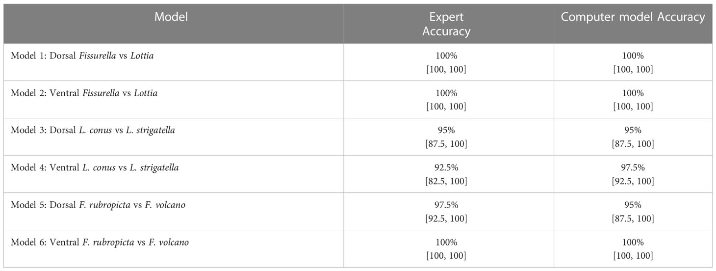
Table 1 Accuracy scores of all trained models with 95% confidence intervals in brackets.
Heatmaps and expert interpretation
After the heatmaps were shown to the experts, they confirmed the following: Across all six models, all the heatmaps were focussed on the specimens (except for one image within model 1 within the Lottia class). Across all six models, all heatmaps appeared to be focussed on specific areas of the shells (except for the same one image in model 1). Heatmaps often focused on a single area of the shells while others focused on multiple features. These features were often common across all images within each respective class (e.g., for the Fissurella class in the genus models 1&2, the focus was always on the keyhole). To review which features were highlighted most frequently, we tallied the responses within the comments made by the experts. For example, if a shell feature/area was focused on in all images from a single class, it would equal 20/20.
Expert opinion: Model 1
For the Fissurella images (Figures 1A–D), 20/20 heatmaps focused on the keyhole. For the Lottia images (Figures 1E–H), 19/20 heatmaps focused on patterns around the shell margin. One heatmap focused its attention around the outside of the shell rather than on it but was still correctly predicted as Lottia. It was noted that the specimens within the Lottia class had a high degree of variable shell patterns and morphology.
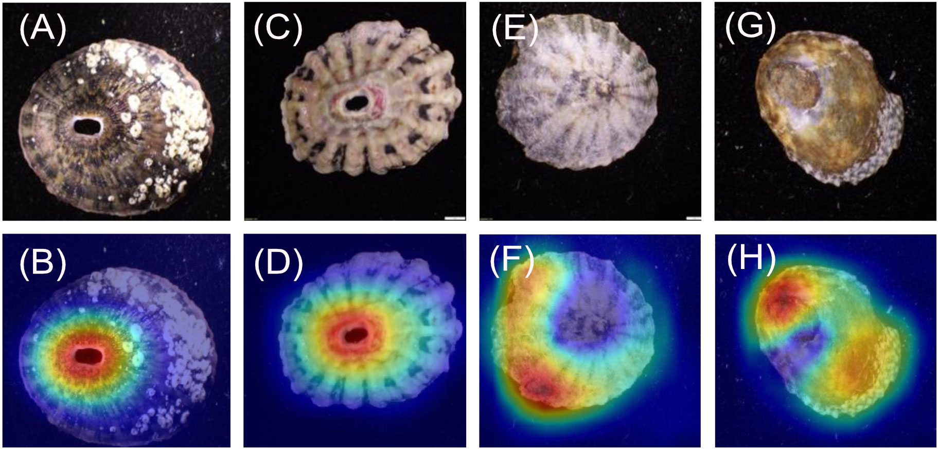
Figure 1 Model 1: Dorsal Fissurella (A–D) vs Lottia (E–H).
Expert opinion: Model 2
For the Fissurella images (Figures 2A–D), 20/20 heatmaps focus on the keyhole. For the Lottia images (Figures 2E–H) 19/20 focused on the areas within the muscle scar and not on the shell margins, while 1/20 focused on the muscle scar to the shell margin.
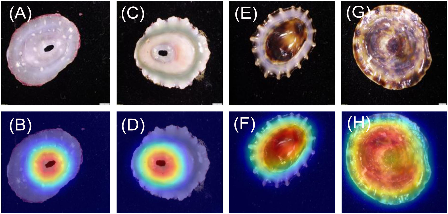
Figure 2 Model 2: Ventral Fissurella (A–D) vs Lottia (E–H).
Expert opinion: Model 3
For the L. conus images (Figures 3A–D), 20/20 heatmaps focus on the ribbing pattern on the shell, but not on the apex. For the L. strigatella images (Figures 3E–H) 17/20 heatmaps focused on the apex, while 3/10 focussed on patterns around the apex.
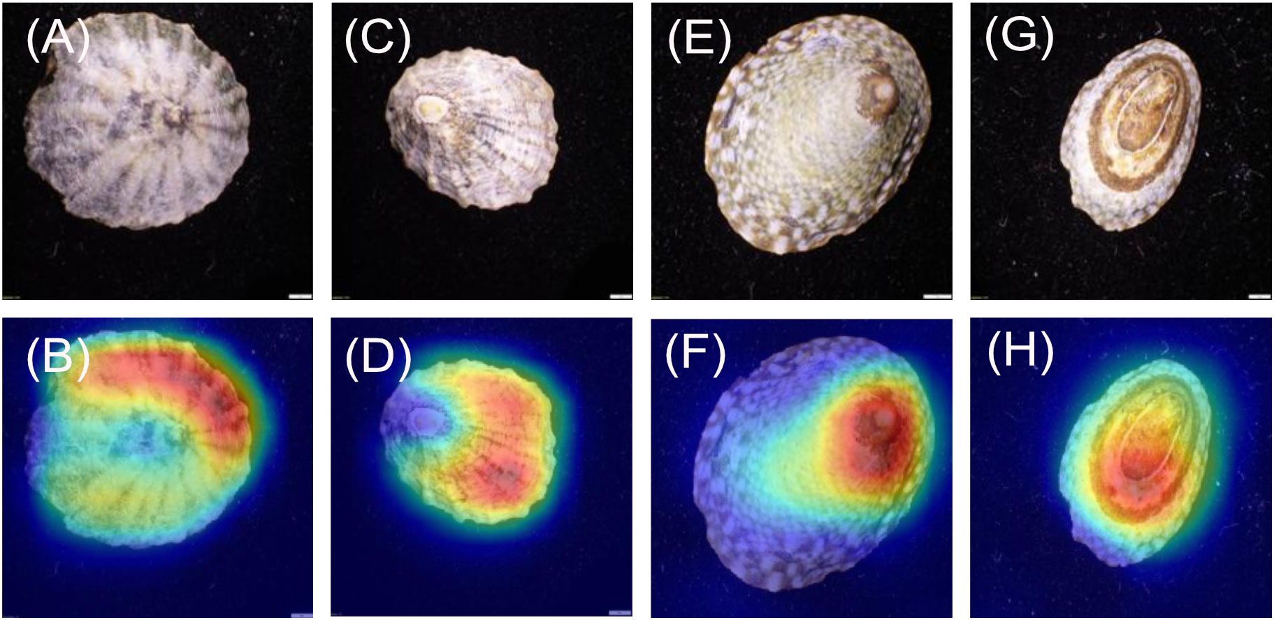
Figure 3 Model 3: Dorsal Lottia conus (A–D) vs Lottia strigatella (E–H).
Expert opinion: Model 4
For the L. conus images (Figures 4A–D), 19/20 heatmaps focus on the area between the muscle scar and the shell margin. 1/20 focused on a very small portion of the shell margin, however, this shell was noted as containing no pattern and was predicted incorrectly (Figure 5). For the L. strigatella images (Figures 4E–H), 20/20 heatmaps focused on areas of the shell margin which is often bordered by a dark or mottled band. Additionally, 2/20 also focused on the centre of the interior portion of the shell within the muscle scar.
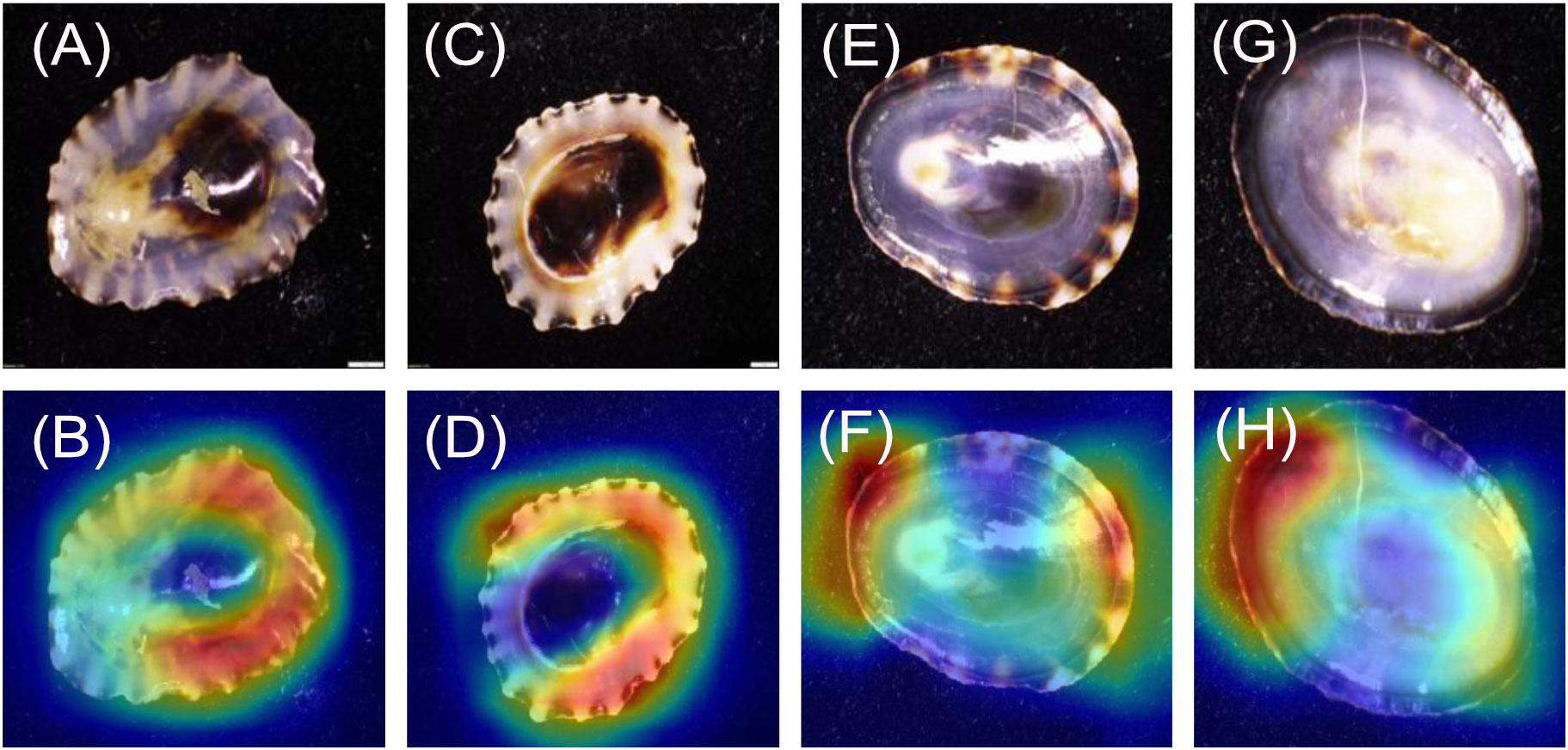
Figure 4 Model 4: Ventral Lottia conus (A–D) vs Lottia strigatella (E–H).
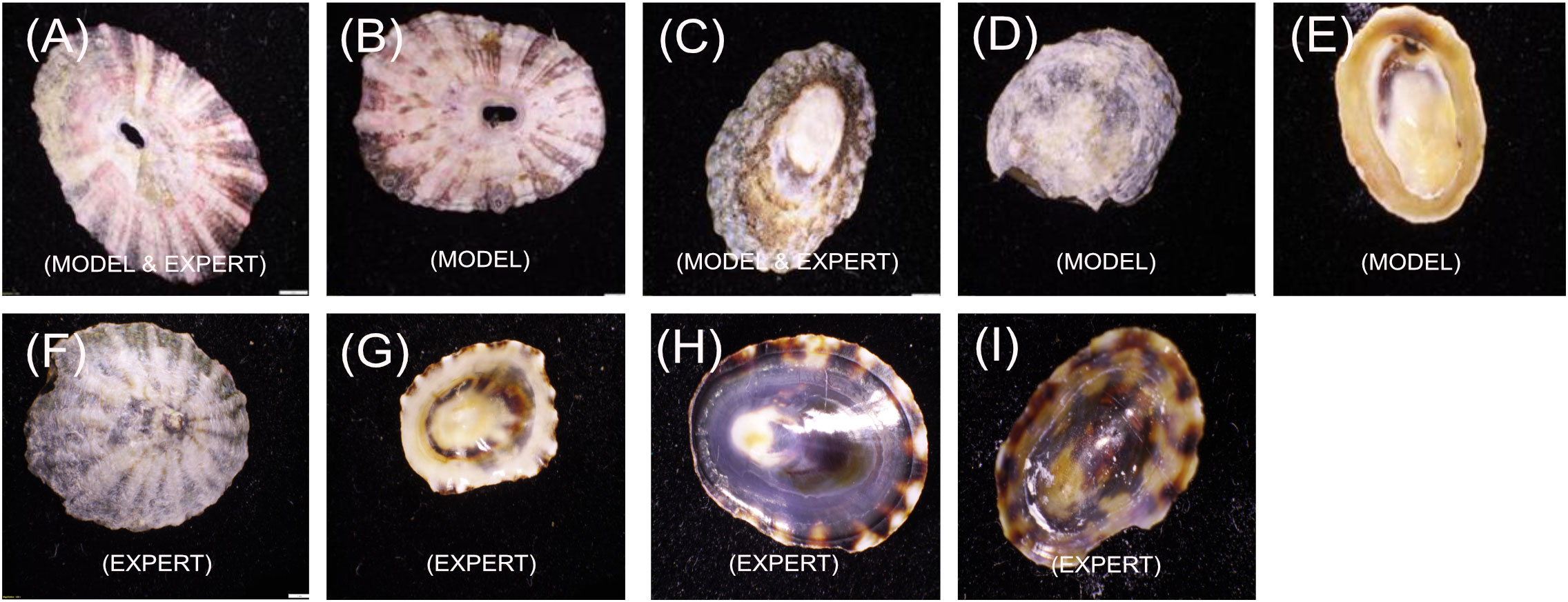
Figure 5 All incorrect model and expert image predictions.
Expert opinion: Model 5
For the F. rubropicta images (Figures 6A–D), 20/20 heatmaps focus on the ribbing pattern on the shell, but not on the keyhole. It was noted that some of the shells were highly eroded but the heatmap still focused on any remaining ribbing patterns. For the F. volcano images (Figures 6E–H) 20/20 heatmaps focused directly on the keyhole. It was noted that the keyhole shape between the two species is different.; F. rubropicta is more lemniscate while F.volcano is ellipsed.
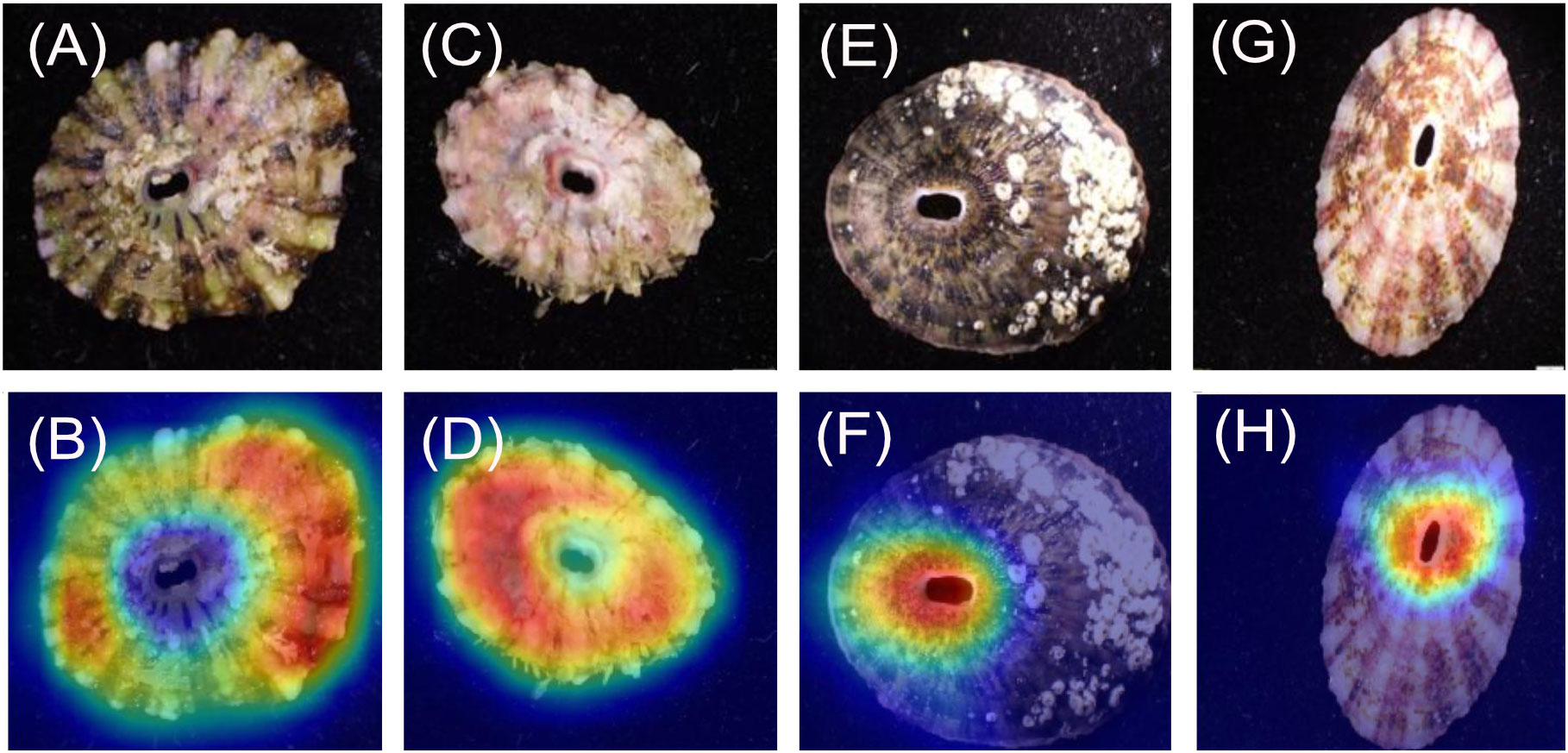
Figure 6 Model 5: Dorsal Fissurella rubropicta (A–D) vs Fissurella volcano (E–H).
Expert opinion: Model 6
For the F. rubropicta images (Figures 7A–D), 20/20 heatmaps focus on the area between the muscle scar and callus (which usually contains a deep red colour) but not on the shell margin. For the F. volcano images (Figures 7E–H) 18/20 heatmaps focused on the margin. 2/20 focused on the margin and on the interior of the shell.
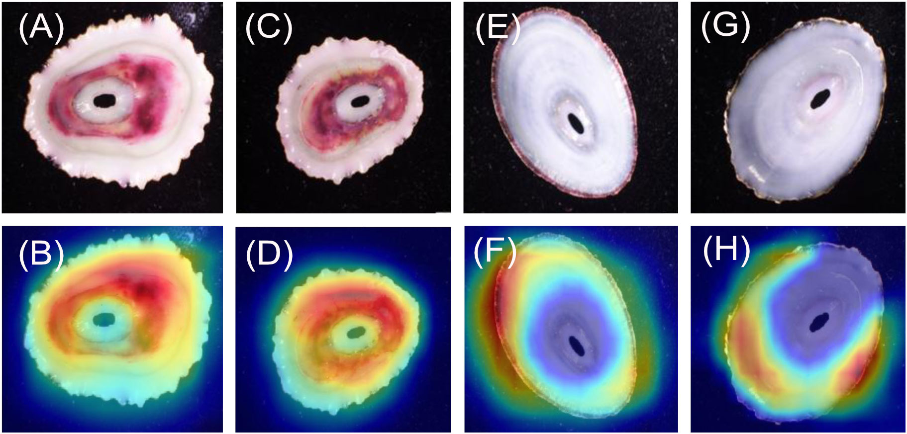
Figure 7 Model 6: Ventral Fissurella rubropicta (A–D) vs Fissurella volcano (E–H).
Incorrect model predictions and expert interpretation
All incorrect model predictions and all incorrect expert predictions (Figure 5) were shown to the experts who were asked to provide an opinion on what morphological features may have caused the misidentification.
Expert opinion: Incorrect model predictions
The F. volcano specimen in Figure 5A was incorrectly predicted by both the model (model 5) and the experts (both incorrectly predicted it as F. rubropicta). Experts determined that this specimen has ribbing patterns normally associated with F. rubropicta. Experts were convinced they were correct but after visual inspection of the ventral side and a correct prediction by the ventral model (6), they concluded that this may just be an outlier individual with dorsal characteristics of both species of Fissurella. In image B, the F. rubropicta specimen was incorrectly predicted by model 5 as F. volcano. Experts determined that this specimen displayed features that they would expect from F. volcano as it has less defined ridging. Image C, an L. conus specimen was incorrectly predicted by model 3 as L. strigatella. This same specimen was also incorrectly predicted by the experts. Upon subsequent inspection, the experts determined that the morphological features of this specimen are not typically associated with L. conus such as not having a banding pattern and the shell pattern is more stippled, which they often attribute to L. strigatella. Image D, an L. strigatella specimen was incorrectly predicted by model 3 as L. conus. The experts determined that the shell is highly eroded and very little morphological information can be used to make a prediction. Image E, a L. conus specimen was incorrectly predicted by model 4 as L. strigatella. Experts determined that it also has very little pattern and largely monochromatic, making it difficult to identify.
Expert opinion: Incorrect expert predictions
Images A and C were incorrectly predicted by both the models and the experts, with reasonings outlined above. Image F is a dorsal view of an L. conus specimen that was incorrectly predicted by the experts as L. strigatella. On reflection, experts commented that they can see some clear L. conus morphological features (clear banding pattern) and were unsure how they incorrectly predicted the specimen initially. Image G is a ventral view of an L. conus specimen that was incorrectly predicted by the experts as L. strigatella. Again, on reflection, experts determined that they could see L. conus features (ribbed margin) and were unsure how they incorrectly predicted the specimen. Image H is a ventral view of an L. strigatella specimen that was incorrectly predicted by the experts as L. conus. On reflection experts determined that the banding pattern around the margin is a feature they would usually associate with L. conus, making this specimen a difficult one to predict (but was correctly predicted by the model). Image I is a ventral view of a L. strigatella specimen and was incorrectly predicted by the experts as L. conus. Experts determined that the pattern on this specimen is unusual and is displaying a tortoiseshell pattern that they could attribute to both Lottia species (the model predicted this specimen correctly).
Heatmap intensity values
For the heatmap intensity values, all models showed a significant difference (P<0.05; two sample Wilcoxon tests) in the mean values between each class (Figure 8). For both genus models (1&2), the Fissurella values are much lower and with a smaller range of values than the Lottia values. For the species comparisons (Figure 8), both the dorsal and ventral views for the Lottia models (3&4) are higher, on average for L. strigatella than L. conus. Likewise, the values for F. rubropicta are on average higher than F. volcano (5&6).
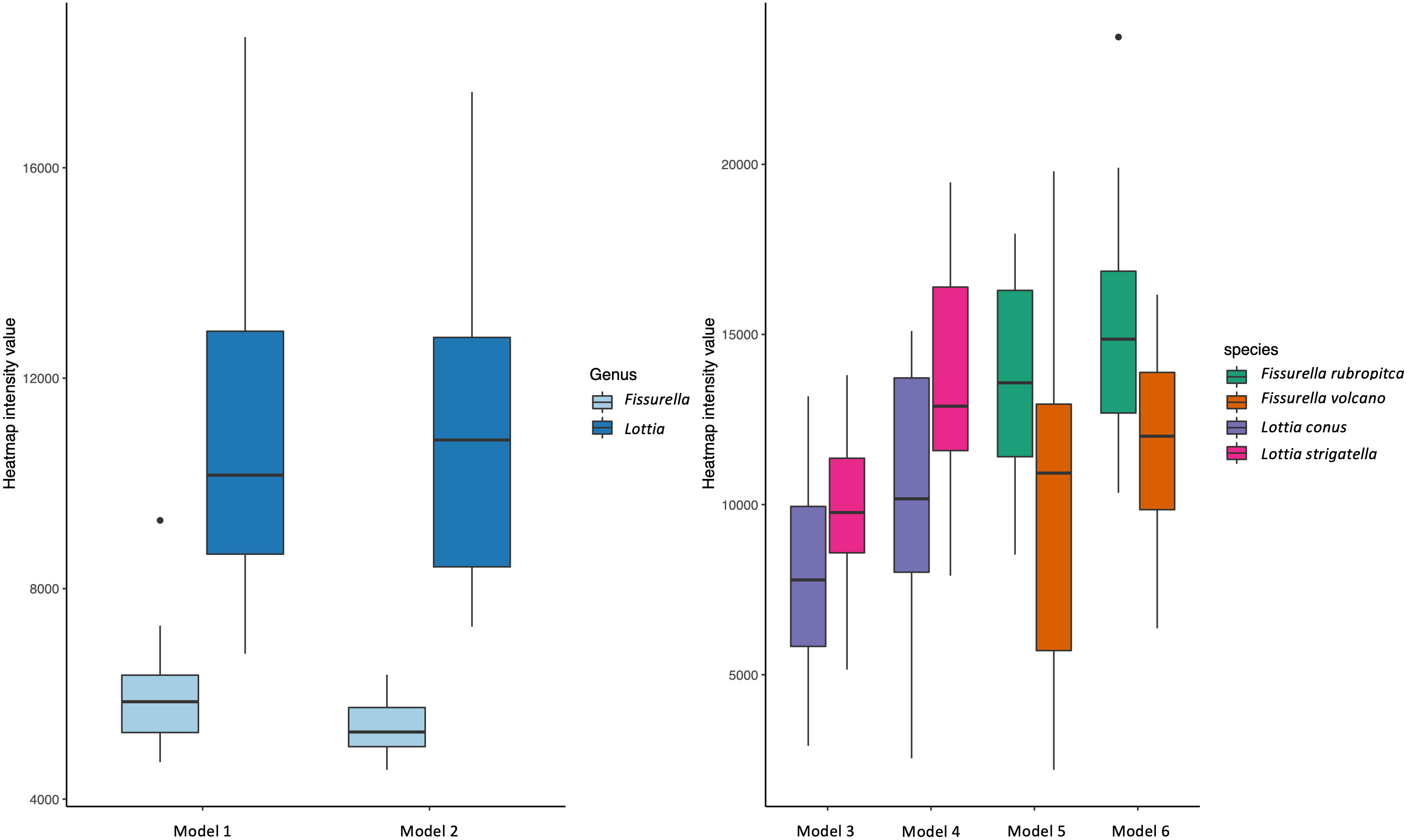
Figure 8 Boxplots showing heatmap intensity values for all models.
Discussion
Computer vision-based limpet identification
The use of CV to help distinguish between species is starting to gain traction amongst ecologists and taxonomists (Wäldchen and Mäder, 2018; Greeff et al., 2022; Hollister et al., 2022). However, few have attempted to pair CV models with heatmaps to help visually distinguish between species with high morphological variability. Limpets, including those species used in this study, can have multiple colour morphs and shell patterns due to several different ecological and life history factors, including substrate type, age, and patterns of shell erosion (Bird, 2011; Williams, 2017). It is therefore not uncommon for field ecologists and museum curators/taxonomists to make mistakes in species identification. To help assist identification, our CV models performed very well and the heatmaps largely focus on shell areas that are morphologically informative between genera and species.
When considering the genera, the models achieved 100% predicted accuracy for the dorsal and ventral orientations (models 1 and 2 respectively). Previous research has shown that higher taxonomic levels tend to score greater than lower levels with computer-based classification problems (Hansen et al., 2020). This is most likely due to having more unique images and having a larger selection of features to associate to each respective class, both of which are shown to improve the performance of CV models (Shorten and Khoshgoftaar, 2019). This follows general taxonomic identification procedures, where higher taxonomic levels are more easily distinguished (Hennig, 1966). It is important to recognise that all Fissurella species have a distinctive keyhole in their shells, whereas true limpets (including Lottia) do not. This is a very clear method of distinguishing the two by eye and the high genus level accuracies evidence this through perfect model performance. This is further supported by the heatmap analysis which clearly shows that the models are focussing on the keyhole of all Fissurella specimens within both models. When viewing the Lottia specimens, the heatmaps are looking at different areas of the specimens, which is reflective of the varied morphology of Lottia. When viewing the heatmap intensity values (Figure 8), the Fissurella class have a much lower mean and spread of values, while the Lottia class has a much higher mean and spread of values. This shows that the models utilise much less visual information to determine the Fissurella class while requiring a lot more information to determine the Lottia class. The experts commented that the keyhole, or a lack of, would be their defining feature to classify either class.
The species vs species models achieved more variable, but still highly accurate results. The ventral oriented models performed better than the dorsal oriented models across both species’ groups. The Lottia ventral model (model 4) performed slightly worse (achieving a prediction accuracy of 97.5%) than the Fissurella ventral model (model 6), which achieved a prediction accuracy score of 100%. However, the Fissurella dorsal model (model 5) and the Lottia dorsal model (model 3) performed equally well (95%). We believe this slight difference in performance between the ventral and dorsal orientations lies in the fact that the dorsal sides will incorporate many factors that can alter appearance, such as erosion and encrusting symbionts that can cover the shell, all of which would hinder the accuracy of CV models. However, the ventral side remains hidden and protected from physical elements. Thus, the ventral side may provide a clearer picture of the differences between species and therefore provide maximum identification opportunities for the CV models. Although this option is not preferable for field identification as the body tissue would need to be removed from shells. Dry shell collections of museum specimens or those collected for other purposes (e.g., population genetics) however, could benefit from the use CV on the ventral and dorsal shell for identification. Again, the heatmap intensity values for the species-based models showed significant differences between each class per model. This suggests that the models found morphological features or areas of similar importance within each class when making their respective predictions. We believe this type of assessment could help researchers interpret decisions made by CV models. For instance, if a prediction does not fit into a known boundary of heatmap intensities for a given class, then it could either be ruled as incorrect or could, at the very least, warrant further investigation, either by revisiting visually by an expert or by molecular means. The heatmap intensity values for the incorrectly predicted specimens (n=5) tend to be lower than the values for the correctly predicted specimens (n=235).
Expert identification and comparison to model performance
Experts performed marginally worse (by one specimen) than the model predictions when considering all images used for the test datasets (n=240). The experts achieved 100% on the genus-based models (models 1 and 2) and the ventral F. rubropicta vs F. volcano (model 6) which is equal to the model performance. The experts performed marginally better on model 5 by 2.5%, performed equally on model 3 and performed worse on model 4. These small differences however are not significant (Table 1). What is striking is the difference in time it takes for the experts and models to make their predictions. It took the experts on average 10 minutes to identify each test set (59 minutes in total) while each model could process their respective test images in less than 6 seconds (30 seconds in total). The experts combined years of limpet-based experience in the study region totals over 22 years, having viewed countless specimens to achieve their personal knowledge base. In contrast, each model used no more than 350 unique images and was created in less than 5 minutes of training time. Therefore, the sheer speed at which CV models can make accurate predictions is one of its primary advantages.
The more unique images that are available for training, then the better the performance of the finished model (Shorten and Khoshgoftaar, 2019). However, at the time of the project, a limited number of specimens were available to create the models, so it is highly likely that if more unique images were available (e.g., from confirmed museum specimens) then we believe that subsequent models could perform even better than those achieved within this project. Interestingly, when viewing the incorrect predictions by themselves, the experts felt that some of their incorrect predictions were a result of human error. A typical downside of the human condition is that performance can decrease due to fatigue or many other cognitive and physical conditions (Mallis et al., 2004), which computers do not suffer. Thus, in the future, we envision that many thousands of specimens can be fed into similar models for identification purposes (e.g., for bulk field collected specimens or un-catalogued museum accessions), alongside confirmation and quality control from expert taxonomists and molecular ecologists.
Heatmap production and expert interpretation
The heatmaps were found to almost always focus upon the specimens, regardless of the model or class. This is a good indicator that the models trained effectively despite the relatively low number of unique images. After the heatmaps were shown to the experts, it was agreed that almost all were focussing on parts of the shell considered to be morphologically important. Occasionally, models focussed on a singular feature, whilst other times they would focus on multiple features. Neither outcome could be considered incorrect. When visually identifying specimens, a human would use a variety of features to make a final decision. However, with cryptic or highly variable species (e.g., some limpet species), the number of defining features is likely to be limited and/or variable among specimens. For instance, the dorsal orientation of L. conus vs L. strigatella can appear similar (model 3), with only a couple of shell characteristics that can be used to distinguish them by eye. In addition, the dorsal side of both shells can be highly eroded making species identification more difficult when only viewed dorsally (e.g., as they are in situ). Regardless, the heatmaps for model 3 appeared to find consistent morphological differences between the species. The L. conus heatmaps mainly focussed on the shell patterns around the apex and looking at shell patterns, while the L. strigatella heatmaps mainly focussed on apex itself. The apex on the dorsal shell of L. strigatella is often highly eroded (Keen, 1971), more so than on L. conus. The apex is the oldest part of the limpet shell, and therefore it is often the most eroded. It is therefore possible that the pattern of shell erosion on the apex is different between the two Lottia species, which may reveal differences in their internal shell structures or microhabitats (Day et al., 2000), but this has not yet been studied in these species.
Again, there are consistent differences between the Lottia species on the ventral sides of their shells. The heatmaps mainly focussed on the area between the muscle scar and the margin areas of the ventral sides of L. conus shells. Whereas on L. strigatella, focussed on the margin perimeter which often contains a dark band.
The dorsal orientations of F. rubropicta vs F. volcano (model 5) heatmaps displayed consistent differences. The F. rubropicta heatmaps consistently focussed on the area around the keyhole/callus, but not on it, while the F. volcano images consistently focussed on the keyhole. The F. rubropicta specimens have more pronounced ribbing on their shells, which the heatmaps appear to focus on. Whereas F. volcano shells are smooth with black/reddish rays. These shell differences may be related to their microhabitat differences: F. volcano are usually found underneath rocks and in sheltered crevices (Morris et al., 1980) while F. rubropicta are exposed and found on top of rocks (PBF and KMZ personal observations). The smooth shells of F. volcano are more suited to life underneath rocks and in crevices, whereas the heavy ribbing of F. rubropicta likely helps reduce water loss (due to higher surface area) during long periods of aerial exposure. Again, the ventral orientation of F. rubropicta vs F. volcano (model 6) heatmaps displayed consistent differences. The F. rubropicta consistently focused on the area within the muscle scar and around the callus, while the F. volcano consistently focused on the margin which usually contains a dark band.
Future considerations
For CV models to be robust, images of accurately identified specimens are required for training purposes. To do this, we relied on DNA barcoding to confirm the species level identifications of the training dataset and to evaluate the accuracy of the test dataset identifications from both the CV models and experts. All specimens were therefore already identified to species level prior to developing the CV models. However, molecular work can be expensive and time consuming. To reduce costs and time, the workflow could be adjusted where only the training dataset are barcoded, and then a smaller sub-sample of specimens in the test dataset could be barcoded to statistically assess the accuracy of the models. Ultimately however, the more specimens that are available for training purposes, the more accurate the model results. If large datasets of confirmed and standardized training images are made publicly available for the known species in a study region, then future researchers could use them to supplement their own training datasets. In particular, we need more training images of the dorsal side of limpet shells, as they are primarily used for field identifications.
More research is also needed to help interpret the utility of heatmaps for understanding ecological questions related to limpet shell morphology (Bird, 2011; Hamilton et al., 2020). With more robust training datasets per species from multiple populations, age/size ranges, and habitat types, we may be able use heatmaps to help decipher if and how shell morphology varies intra-specifically over local to regional scales. For example, the intensity and location of heatmaps may differ based on factors such as: microhabitat, population, size/age, and region. We can then use this information to shed new light on how and why limpet shells have such high morphological variability (Giesel, 1970).
Conclusion
This project demonstrates the effectiveness of using CV in identifying limpets based on images of their shells. Despite the variable shell morphologies and colour patterns within and between species, the CV models were able to classify them to genus (100%) and species level (95% - 100%) with high accuracy and quickly, even with small datasets. The use of heatmaps confirmed that the models were focusing on the limpet shells, and when reviewed by expert taxonomists, they agreed that the heatmaps highlighted significant and unique morphological features for each genus and species.
Typically, DL models are considered as ‘black box’ systems due to their complex decision-making processes and the ‘impossibility’ of truly understanding how these types of systems come to their final conclusions. However, the use of heatmaps offers a means to understand how CV makes its decisions. The results show that the models can differentiate between visually similar species or those with high morphological variability, and that they utilize unique morphological features to distinguish them. In the future, we envision this type of system being used by taxonomists as a tool to assist them in identifying important or new morphological features to help distinguish between visually similar and cryptic species. Additionally, similar methods could assist with field identification of limpets and potentially replace the need to collect numerous specimens purely for identification purposes. Computer models, once trained, require far less computation power to perform identifications, and most can be uploaded and used from a modern mobile phone.
It is important to consider the strengths and limitations of CV models for identification purposes. No single method is perfect, but combining the strengths of CV, molecular methods, and human expertise will allow us to gain new insights for taxonomy and ecology. Not only for limpets, but for all of biodiversity.
Data availability statement
The original contributions presented in the study are included in the article/supplementary material. Further inquiries can be directed to the corresponding author.
Ethics statement
The animal study was reviewed and approved by Animal Welfare and Ethical Review Body - ERGO II 63575.
Author contributions
JH, took images of limpets, wrote model code, ran CV models, produced heatmaps, wrote bulk of paper, consulted with morphology analysis. PF, collected samples from field, assisted heavily with writing of paper, gave expert opinion on morphology analysis. KZ, collection samples from field, identified using molecular methods, gave expert opinion of morphology analysis, comment on and edited final drafts. BP, commented on and edited final drafts. TH, commented on and edited final drafts. XC, commented on CV methods, commented on and edited final drafts. All authors contributed to the article and approved the submitted version.
Acknowledgments
We would like to thank Moira Maclean and David Paz García for their assistance with fieldwork and specimen collection. We would like to thank the University of Southampton, the National Oceanography centre, and the Natural History Museum for their assistance with additional equipment needs. JDH and KMZ would like to thank NERC and the INSPIRE doctoral training programme for funding portions of this research. PBF acknowledges funding from NERC grant: NE/X011518/1. We would like to thank Sanson Poon from the Natural History Museum for his consultations for appropriate statistical evaluations for this paper.
Conflict of interest
The authors declare that the research was conducted in the absence of any commercial or financial relationships that could be construed as a potential conflict of interest.
Publisher’s note
All claims expressed in this article are solely those of the authors and do not necessarily represent those of their affiliated organizations, or those of the publisher, the editors and the reviewers. Any product that may be evaluated in this article, or claim that may be made by its manufacturer, is not guaranteed or endorsed by the publisher.
Footnotes
- ^ Zarzyczny, K. M., Hellberg, M. E., Lugli, E. B., Maclean, M., García, D. P., Rius, M., et al. (under minor revision). Tropicalisation and phylogeographic structure of rocky shore gastropods on the Baja California Peninsula
References
Bird C. E. (2011). Morphological and behavioral evidence for adaptive diversification of sympatric Hawaiian limpets (Cellana spp.). Integr. Comp. Biol. 51, 466–473. doi: 10.1093/icb/icr050
Burdi C. (2015). A test of diagnostic shell differences of the limpets Lottia conus and Lottia scabra identified with PCR-based assay. Masters dissertation. (California State University, Fullerton).
Carpenter P. P. (1864). XXXII.—Diagnoses of new forms of mollusks collected at Cape St. Lucas by Mr. J. Xantus. Ann. Magazine Natural History 13, 311–315. doi: 10.1080/00222936408681615
Crummett L. T., Eernisse D. J. (2007). Genetic evidence for the cryptic species pair, Lottia digitalis and Lottia austrodigitalis and microhabitat partitioning in sympatry. Mar. Biol. 152, 1–13. doi: 10.1007/s00227-007-0621-4
Dawson M. N., Hays C. G., Grosberg R. K., Raimondi P. T. (2014). Dispersal potential and population genetic structure in the marine intertidal of the eastern North Pacific. Ecol. Monogr. 84, 435–456. doi: 10.1890/13-0871.1
Day E. G., Branch G. M., Viljoen C. (2000). How costly is molluscan shell erosion? A comparison of two patellid limpets with contrasting shell structures. J. Exp. Mar. Biol. Ecol. 243, 185–208. doi: 10.1016/S0022-0981(99)00120-3
Fenberg P. B., Roy K. (2008). Ecological and evolutionary consequences of size-selective harvesting: how much do we know? Mol. Ecol. 17, 209–220. doi: 10.1111/j.1365-294X.2007.03522.x
Fenberg P. B., Roy K. (2012). Anthropogenic harvesting pressure and changes in life history: insights from a rocky intertidal limpet. Am. Nat. 180, 200–210. doi: 10.1086/666613
Firth L. B. (2021). What have limpets ever done for us?: On the past and present provisioning and cultural services of limpets. Int. Rev. Environ. History 7, 5–45. doi: 10.22459/IREH.07.02.2021.01
Giesel J. T. (1970). On the maintenance of a shell pattern and behavior polymorphism in Acmaea digitalis, a limpet. Evolution 24, 98–119. doi: 10.1111/j.1558-5646.1970.tb01743.x
Greeff M., Caspers M., Kalkman V., Willemse L., Sunderland B. D., Bánki O., et al. (2022). Sharing taxonomic expertise between natural history collections using image recognition. Res. Ideas Outcomes 8, e79187. doi: 10.3897/rio.8.e79187
Hamilton A. M., Selwyn J. D., Hamner R. M., Johnson H. K., Brown T., Springer S. K., et al. (2020). Biogeography of shell morphology in over-exploited shellfish reveals adaptive trade-offs on human-inhabited islands and incipient selectively driven lineage bifurcation. J. Biogeogr. 47, 1494–1509. doi: 10.1111/jbi.13845
Hansen O. L., Svenning J. C., Olsen K., Dupont S., Garner B. H., Iosifidis A., et al. (2020). Species-level image classification with convolutional neural network enables insect identification from habitus images. Ecol. Evol. 10, 737–747. doi: 10.1002/ece3.5921
Hollister J., Vega R., Azhar M. H. B. (2022). Automatic identification of non-biting midges (Chironomidae) using object detection and deep learning techniques. ICPRAM 1, 256–263. doi: 10.5220/0010822800003122
Høye T. T., Ärje J., Bjerge K., Hansen O. L., Iosifidis A., Leese F., et al. (2021). Deep learning and computer vision will transform entomology. Proc. Natl. Acad. Sci. 118, e2002545117. doi: 10.1073/pnas.2002545117
Joshi S., Owens J. A., Shah S., Munasinghe T. (2021). Analysis of preprocessing techniques, Keras tuner, and transfer learning on cloud street image data. 2021 IEEE International Conference on Big Data (Big Data), Orlando, FL, USA, 4165–4168.
Keen A. M. (1971). Sea Shells of Tropical West America: Marine Mollusks from Baja California to Peru (Stanford: Stanford University Press).
Kordas R. L., Donohue I., Harley C. D. G. (2017). Herbivory enables marine communities to resist warming. Sci. Adv. 3, e1701349. doi: 10.1126/sciadv.1701349
Kuo E. S., Sanford E. (2013). Northern Distribution of the Seaweed Limpet Lottia insessa (Mollusca: Gastropoda) along the Pacific Coast. Pacific Sci. 67, 303–313. doi: 10.2984/67.2.12
Lürig M. D. (2022). Phenopype: a phenotyping pipeline for Python. Methods Ecol. Evol. 13, 569–576. doi: 10.1111/2041-210X.13771
Mallis M. M., Mejdal S., Nguyen T. T., Dinges D. F. (2004). Summary of the key features of seven biomathematical models of human fatigue and performance. Aviation Space Environ. Med. 75, 4–14.
Morris R. H., Abbott D. P., Haderlie E. C. (1980). Intertidal invertebrates of California (Stanford: Stanford University Press).
Nakano T., Spencer H. G. (2007). Simultaneous polyphenism and cryptic species in an intertidal limpet from New Zealand. Mol. Phylogenet. Evol. 45, 470–479. doi: 10.1016/j.ympev.2007.07.020
Perez L., Wang J. (2017). The effectiveness of data augmentation in image classification using deep learning. arXiv:1712.04621v1. doi: 10.48550/arXiv.1712.04621
Pilsbry H. (1890). Manual of conchology, structural and systematic, with illustrations of the species. 1(12): Stomatellidae, Scissurellidae, Pleurotomariidae, Haliotidae, Scutellinidae, Addisoniidae, Cocculinidae, Fissurellidae (Philadelphia: Conchological Section, Academy of Natural Sciences).
Pinho C., Kaliontzopoulou A., Ferreira C. A., Gama J. (2022). Identification of morphologically cryptic species with computer vision models: wall lizards (Squamata: Lacertidae: Podarcis) as a case study. Zoological J. Linn. Soc. 198, 184–201. doi: 10.1093/zoolinnean/zlac087
Popov D., Roychoudhury P., Hardy H., Livermore L., Norris K. (2021). The value of digitising natural history collections. Res. Ideas Outcomes 7, e78844. doi: 10.3897/rio.7.e78844
Rädsch T., Reinke A., Weru V., Tizabi M. D., Schreck N., Kavur A. E., et al. (2023). Labelling instructions matter in biomedical image analysis. Nat. Mach. Intell. 5, 273–283. doi: 10.1038/s42256-023-00625-5
Reeve L. (1849). “Monograph of the genus Fissurella,” in Conchologia Iconica, or, illustrations of the shells of molluscous animals (London: Reeve & Co).
Rogers A. J., Weisler M. I. (2020a). Assessing the efficacy of genus-level data in archaeomalacology: A case study of the Hawaiian limpet (Cellana spp.), Moloka ‘i, Hawaiian islands. J. Island Coast. Archaeol. 15, 28–56. doi: 10.1080/15564894.2018.1481467
Rogers A. J., Weisler M. I. (2020b). Limpet (Cellana spp.) shape is correlated with basalt or eolianite coastlines: Insights into prehistoric marine shellfish foraging and mobility in the Hawaiian Islands. J. Archaeological Sci.: Rep. 34, 102561. doi: 10.1016/j.jasrep.2020.102561
Ross E. (2022). Phylogeography of the cryptic intertidal gastropod Lottia conus along the Pacific coast from Southern California to Central Mexico. Masters Dissertation. (University of Southampton).
Savage N. (2022). Breaking into the black box of artificial intelligence. Nature. doi: 10.1038/d41586-022-00858-1
Selvaraju R., Cogswell M., Das A., Vedantam R., Parikh D., Batra D. (2016). "Grad-CAM: Visual Explanations from Deep Networks via Gradient-Based Localization,", 2017 IEEE International Conference on Computer Vision (ICCV), (Venice, Italy) 618–626. doi: 10.1007/s11263-019-01228-7
Sham A. H., Aktas K., Rizhinashvili D., Kuklianov D., Alisinanoglu F., Ofodile I., et al. (2022). Ethical AI in facial expression analysis: racial bias. Signal Image Video Process. 17, 1–8. doi: 10.1007/s11760-022-02246-8
Shorten C., Khoshgoftaar T. M. (2019). A survey on image data augmentation for deep learning. J. Big Data 6, 1–48. doi: 10.1186/s40537-019-0197-0
Simison W. B., Lindberg D. R. (1999). Morphological and molecular resolution of a putative cryptic species complex: a case study of Notoacmea fascicularis (Menke 1851)(Gastropoda: Patellogastropoda). J. Molluscan Stud. 65, 99–109. doi: 10.1093/mollus/65.1.99
Simison W. B., Lindberg D. R. (2003). On the identity of Lottia strigatella (Carpenter 1864)(Patellogastropoda: Lottiidae). Veliger 46, 1–19.
Simonyan K., Zisserman A. (2014). Very deep convolutional networks for large-scale image recognition. arXiv:1409:1556. doi: 10.48550/arXiv.1409.1556
Tamura K., Stecher G., Kumar S. (2021). MEGA11: molecular evolutionary genetics analysis version 11. Mol. Biol. Evol. 38, 3022–3027. doi: 10.1093/molbev/msab120
Tautz D., Arctander P., Minelli A., Thomas R. H., Vogler A. P. (2003). A plea for DNA taxonomy. Trends Ecol. Evol. 18, 70–74. doi: 10.1016/S0169-5347(02)00041-1
Wäldchen J., Mäder P. (2018). Machine learning for image based species identification. Methods Ecol. Evol. 9, 2216–2225. doi: 10.1111/2041-210X.13075
Weisler M. I., Rogers A. J. (2021). Ritual use of limpets in late Hawaiian prehistory. J. Field Archaeol. 46, 52–61. doi: 10.1080/00934690.2020.1835267
Wilson R. J., De Siqueira A. F., Brooks S. J., Price B. W., Simon L. M., van der Walt S. J., et al. (2022). Applying computer vision to digitised natural history collections for climate change research: Temperature-size responses in British butterflies. Methods Ecol. Evol. 14, 372–384. doi: 10.1111/2041-210X.13844
Keywords: Baja California, computer vision, convolutional neural network, heatmap, limpets, rocky intertidal, taxonomy
Citation: Hollister JD, Cai X, Horton T, Price BW, Zarzyczny KM and Fenberg PB (2023) Using computer vision to identify limpets from their shells: a case study using four species from the Baja California peninsula. Front. Mar. Sci. 10:1167818. doi: 10.3389/fmars.2023.1167818
Received: 16 February 2023; Accepted: 07 July 2023;
Published: 27 July 2023.
Edited by:
Tomoyuki Nakano, Kyoto University, JapanReviewed by:
Marshall Weisler, The University of Queensland, AustraliaYunwei Dong, Ocean University of China, China
Copyright © 2023 Hollister, Cai, Horton, Price, Zarzyczny and Fenberg. This is an open-access article distributed under the terms of the Creative Commons Attribution License (CC BY). The use, distribution or reproduction in other forums is permitted, provided the original author(s) and the copyright owner(s) are credited and that the original publication in this journal is cited, in accordance with accepted academic practice. No use, distribution or reproduction is permitted which does not comply with these terms.
*Correspondence: Jack D. Hollister, jdh2n21@soton.ac.uk