- State Key Laboratory of Marine Geology, Tongji University, Shanghai, China
The ultraviolet absorption spectra of chromophoric dissolved organic matter (CDOM) can be used to trace its sources and to explore the dynamic of the CDOM pool. In previous studies, only the spectra above 240 nm can be used directly to characterize the CDOM in seawater, due to the overlapping of CDOM absorption spectra below 240 nm with inorganic chemicals such as , , Cl- and Br-. In this study, three different machine learning models, back propagation neural network (BPNN), random forest (RF) and extreme gradient boosting (XGBoost), were built to predict the CDOM ultraviolet absorption spectra between 215 and 350 nm after being trained with the raw absorption spectra of seawater. The optimal input wavelength range of the raw seawater spectra is 250-350 nm, and the optimal model parameters of machine learning algorithms were determined by using five-fold cross validation. The results show that the three models can well predict the CDOM absorption spectra. Comparatively, the XGBoost model gave the best prediction results. The reasons might be related to the fact that the XGBoost algorithm focuses on the residuals generated by the last iteration, which can reduce both variance and bias, especially for datasets with small sample sizes. Based on the predicted spectra by XGBoost algorithm, we calculated the spectra slopes of short wavelengths between 215 and 240 nm (S215-240) and between 215 and 275 nm (S215-275). The results show that the S215-240 and S215-275 are ~2 times the widely used spectra slopes between 275 and 295 nm (S275-295) obtained by traditional method based on the raw spectra. Moreover, the S215-240 and S215-275 are more relavant with salinity for marine CDOM than S275-295, suggesting spectra slopes of shorter wavelengths might be the better proxies for marine CDOM than that of longer wavelengths.
1 Introduction
Chromophoric dissolved organic matter (CDOM), which is also called yellow substance, widely exists in oceans, lakes and rivers. It plays a key role in climate-related biogeochemical cycles in aquatic ecosystems, such as carbon dynamics, phytoplankton activity, microbial growth and ecosystem productivity (Nelson and Siegel, 2013; Stedmon and Nelson, 2015). CDOM is a soluble and complex mixture of many kinds of organic substances, including humic acid, fulvic acid and aromatic polymers (Li and Hur, 2017; Zhang et al., 2021), which constitutes a significant fraction of the DOM pool in natural waters (10 ~ 90%) (Twardowski et al., 2004). CDOM can absorb both ultraviolet and visible (UV-Vis) light and it is well known that the optical properties of CDOM in seawater can be used to trace its sources and to explore the dynamic of the CDOM pool (Whitehead et al., 2000; McKnight et al., 2001; Stedmon and Markager, 2001; Baker and Spencer, 2004; Guo et al., 2007; Yang et al., 2013; Yamashita et al., 2013; Jørgensen et al., 2014). However, due to the complexity of CDOM compositions, it is difficult to link the optical absorbance directly to CDOM concentrations or its chemical compositions (Del Castillo and Coble, 2000; Zhao et al., 2018; Nima et al., 2019). Since the UV-Vis absorption spectra of CDOM decrease approximately exponentially with increasing wavelength, exponential models are generally used to describe CDOM absorption spectra (Stedmon and Markager, 2001; Twardowski et al., 2004; Helms et al., 2008; Li and Hur, 2017). The most often used model is given in Equation (1).
where λ is the wavelength (nm), λ0 is a reference wavelength (nm), ACDOM(λ) and ACDOM(λ0) are the CDOM absorbance at the wavelength of λ and λ0, k is a background constant (m-1), S is the spectral slope (nm-1) that describes the approximate exponential rate of decrease in absorption with increasing wavelengths.
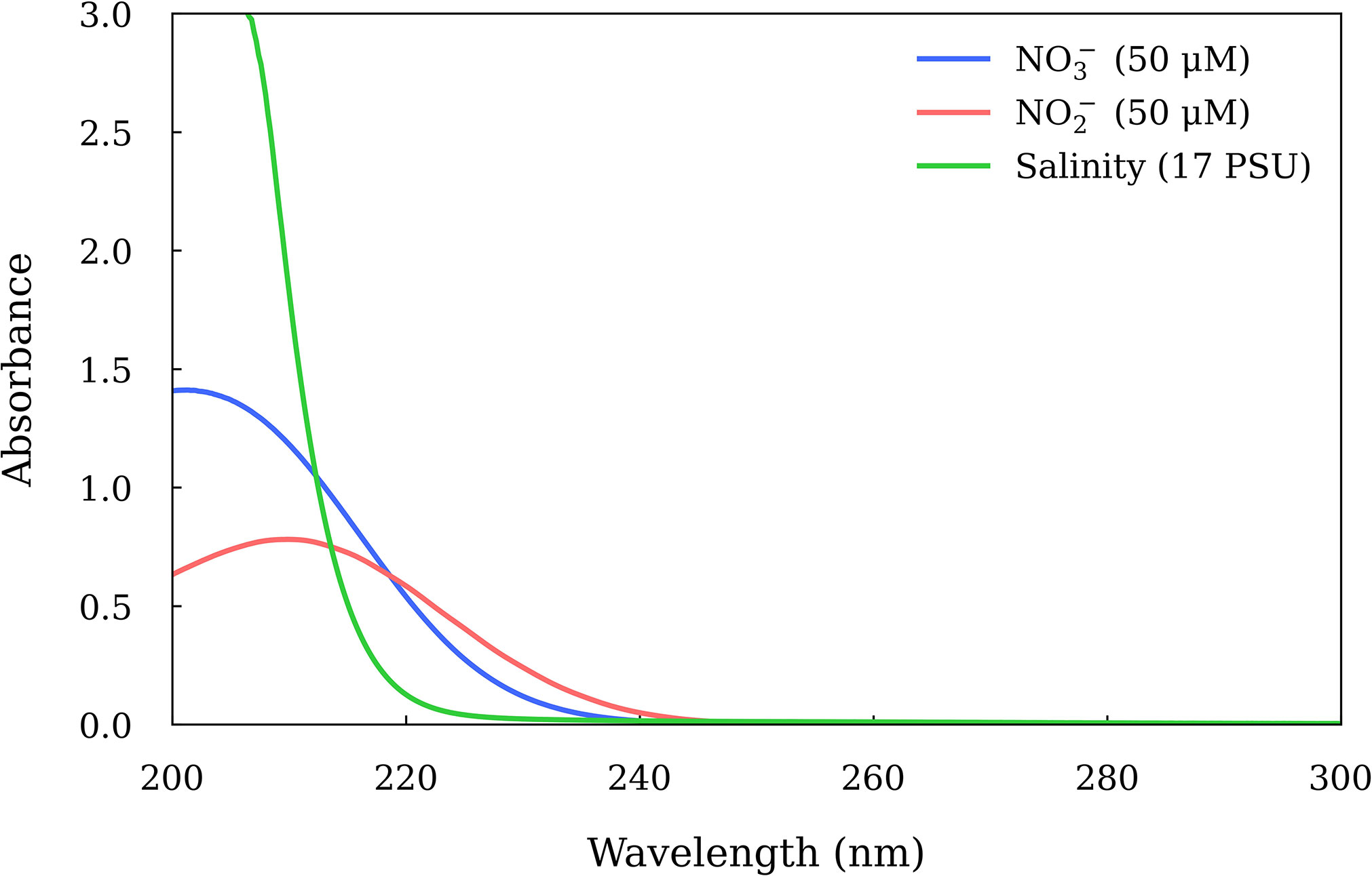
The S, k and Equation (1) for characterizing different CDOM are usually obtained over the wavelength ranges of > 275 nm (e.g., 275-295, 350-400 and 300-600 nm) (Twardowski et al., 2004; Li and Hur, 2017). Only recently, Massicotte and Markager (2016) used a Gaussian decomposition approach to model CDOM absorption spectra between 240 and 700 nm, which can remove the errors associated with the choice of the spectral range used to estimate S. However, the spectra below 240 nm can’t be modelled directly using Equation (1), because several inorganic ions in seawater including , Cl- and Br- have strong absorbance between 190 and 250 nm (Figure 1), which overlap with that of CDOM (Guenther et al., 2001; Johnson and Coletti, 2002). Vice versa, when measuring and by ultraviolet spectroscopic method, CDOM would interfere with the analyzing results (Armstrong, 1963; Johnson and Coletti, 2002; Sakamoto et al., 2009). Therefore, unraveling the CDOM UV absorbance below 240 nm can improve the understanding of CDOM light absorbance characteristics and help to determine and concentrations in seawater accurately when using spectroscopic techniques.
Machine learning algorithms can cope with nonlinearity and other complex regression problems (Verrelst et al., 2012). In the last decade, machine learning techniques have been increasingly employed to estimate CDOM abundance and trace their sources and reactivity. However, most of these studies built machine learning models based on CDOM fluorescence spectroscopy (Stedmon et al., 2003; Stedmon and Bro, 2008; Murphy et al., 2008; Nelson and Gauglitz, 2016; Murphy et al., 2018; Sun et al., 2022), which can provide rich information with its three-dimensional data (i.e. excitation, emission and intensity) (Stedmon et al., 2003; Stedmon and Bro 2008; Coble et al., 2014; Murphy et al., 2018; Marín-García and Tauler, 2020). In addition, many scholars have developed algorithms based on remotely sensed reflectance to characterize CDOM (Cao and Miller, 2015; Ruescas et al., 2018; Zhao et al., 2018), although it is difficult to obtain an accurate estimation of CDOM from satellite data due to its low optical signals and absorption spectral shapes that are similar to those of nonphytoplankton particulate matter (Zhang et al., 2021). To data, there are no reports on CDOM UV-Vis spectra below 240 nm combined with machine learning models.
In this work, we aim to model the UV-Vis absorption spectra of CDOM in seawater between 215 and 350 nm by machine learning models based on the raw absorption spectra of seawater. Three machine learning algorithms, back propagation neural network (BPNN), random forest (RF) and extreme gradient boosting (XGBoost), were implemented to establish the prediction models. The optimal input wavelength range and model parameters were selected and the results from the three algorithms were evaluated and compared.
2 Materials and methods
2.1 Apparatus
A UV-Vis spectrophotometer (Specord plus 210, Analytik Jena AG, Germany) was used to collect absorption spectra of seawater from 200 to 350 nm. All the samples were measured in a 3.0 cm quartz cuvette with spectral resolution set to 0.2 nm. The script programs for the XGBoost, RF and BPNN algorithms were written based on python language.
2.2 Data preprocessing
2.2.1 Dataset
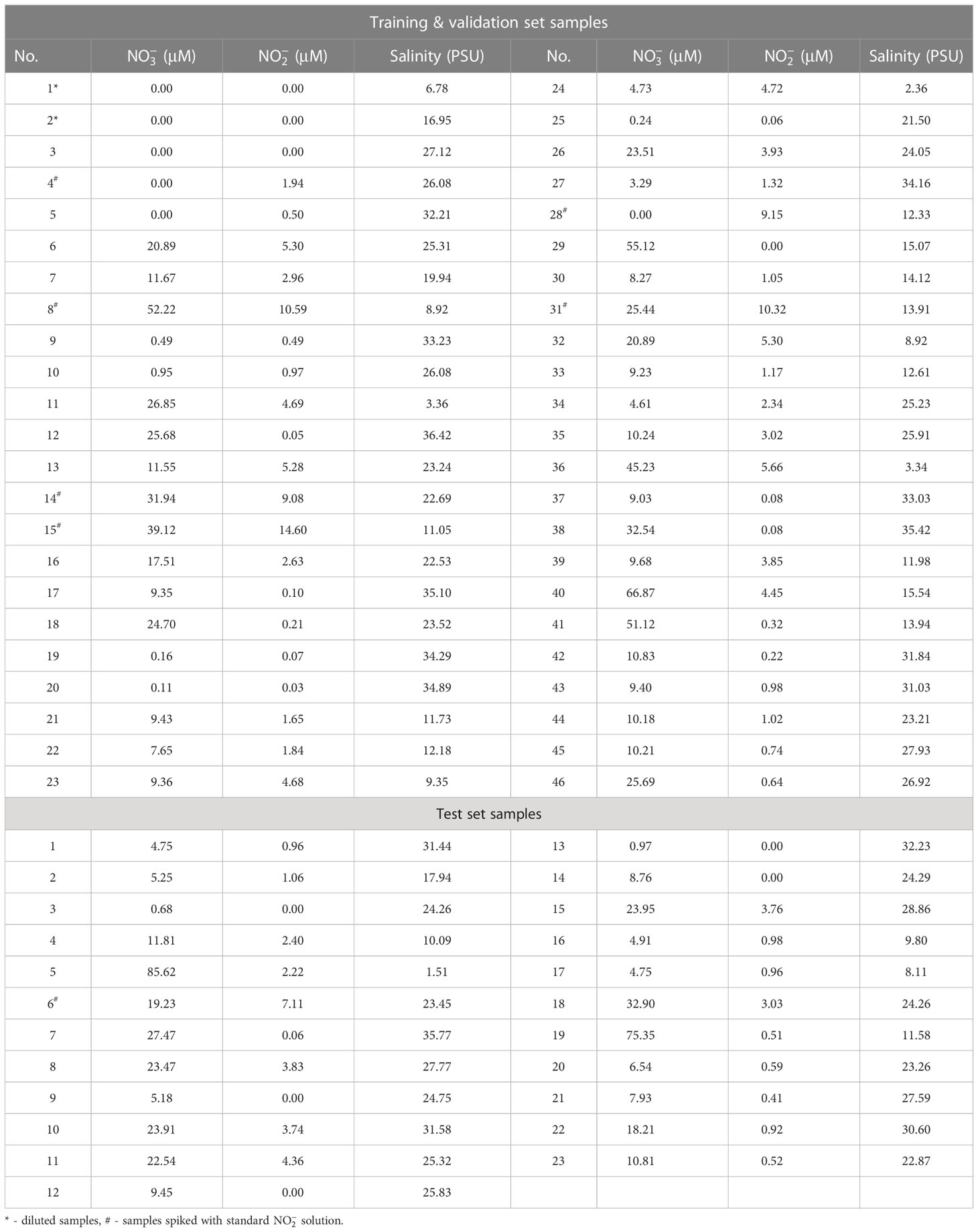
Water samples with different , and CDOM concentrations and salinities were collected from the Changjiang River Estuary and East China Sea. These samples were split into a training and test set at a ratio of 2:1, and 20% of the training set samples were randomly taken as validation set. Notably, the splitting ratio of training and test sets can be 3:1 or 4:1, etc according to the number of samples. While selecting the samples, care was taken to include one-, two- and three-component of , and salinity with various concentrations in the training set in order that the built models have better prediction performance (Mitchell, 1997; Quinonero-Candela et al., 2008). Hence, several natural seawater samples were diluted by Milli-Q water or added by standard solutions considering the very low concentrations in samples compared with (Table 1). The resulting and concentrations and salinities in the training set ranged from 0 to 85.62 μM, 0 to 14.60 μM and 0 to 35.42 PSU (practical salinity units), respectively (Table 1), which can cover their concentrations in the Changjiang River Estuary and East China Sea.
2.2.2 Calculation of the theoretical CDOM absorption spectra
In seawater, the main inorganic and organic chemical substances absorbing UV light include , salinity and CDOM. As a result, the CDOM absorbance can be obtained from the difference between the total seawater absorbance (Aλ) and the absorbance of and salinity ( , , Asalinity ), which can be shown in Equation (2). Based on the Beer-Lambert law, Equation (2) can be changed to Equation (3).
Where b is the path length (cm) of the optical cell, ϵ is the absorption coefficient of the subscripted species (l mol-1 m-1 for and , PSU-1 m-1 for salinity), C is the concentration of the subscripted species. Each ϵ value can be obtained by measuring the absorption in the standard solutions with known concentrations. and concentrations were measured by conventional wet-chemical analyses (colorimetric Griess assay) using an AA3 Auto-Analyzer (Bran Luebbe Co., Germany). was determined using the pink azo dye spectrophotometric method at wavelength of 543 nm. was first reduced to using a cadmium column before measurement. Salinity values of the samples were from an in-situ conductivity-temperature-depth (CTD) recorder (SBE911, Sea-Bird Co., USA) onboard.
2.3 Machine learning algorithms
2.3.1 BPNN
BPNN is a multi-layer feedforward artificial neural network trained by error back propagation algorithm (Rumelhart and McClelland, 1986; Zhou and Li, 2020). It consists of input layer, hidden layer and output layer. In BPNN, considering the neurons between different layers are inter-connected, each layer is also called as a fully connected (FC) layer, which can combine the features from the previous layer (Hecht-Nielsen, 1992; Erb, 1993; Li et al., 2012; Tawfik et al., 2018). BPNN uses activation functions to accomplish nonlinear data transformation, which is added to the FC layer and allows the network to create arbitrary nonlinear complex mappings between inputs and outputs. The commonly used activation functions include sigmoid and ReLU, which are shown in Equations (4) and (5).
The BPNN model is trained by continuously adjusting the weights and thresholds of each neuron, and the training processes consist forward propagation and backward feedback. The former transmits the output values layer by layer, while the latter sums the error derivatives for weights in the reverse direction until all the data are run through the network once (Dong et al., 2020). This constitutes an epoch, and the weights are updated after each epoch such that the model error decreases (Primadusi et al., 2016).
In this paper, the input, output and the theoretical output of BPNN model are respectively x = (x1, x2, ···, xn), y = (y1, y2, ···, ym) and d = (d1, d2,···, dm). The xn represents the n-th wavelength of the input raw seawater spectra, the ym and dm represent the m-th wavelength of the calculated and theoretical output CDOM spectra, respectively.
2.3.2 RF
As an ensemble learning method, RF creates multiple decision classification trees with random subsets of the original training dataset (Breiman, 2001; Cutler et al., 2012). By averaging the predictions of each decision tree, RF can get a more accurate result. The training subset of each tree is generated by a bootstrapping procedure, which divides the training dataset into an “in-bag” subset for the training of the decision tree and an “out-of-bag” subset not included in the training process. This partitioning is unique for each tree in the forest and hence provides a significant internal validation. As a result, RF can overcome the disadvantages of overfitting and instability and has good robustness and high interpretability (Khoshgoftaar et al., 2007; Primadusi et al., 2016). More specific details of RF algorithm can be found in Breiman’ article (Breiman, 2001).
Here, the samples in the training set are randomly sampled repeatedly by bootstrap resampling technology to generate K sub-training sets, and each sub-training set constructs a regression tree. The prediction result of CDOM spectrum in the i-th seawater sample can be calculated as follows:
Where xi, j denotes the input raw seawater spectra of the i-th sample in the j-th sub-training set, θj is the random variable of the j-th regression tree, y(xi,j,θj ) represents the predicted CDOM spectra of the j-th regression tree for the i-th sample.
2.3.3 XGBoost
XGBoost is an improved algorithm based on gradient boosting decision tree. It is developed to increase the computing speed and accuracy, and thus require less training and prediction time. Instead of averaging independent trees, XGBoost recursively adds decision trees that are created from the prediction errors or residuals of the previous tree model until no significant improvement is detected (Abdel-Rahman et al., 2017). Unlike RF, where the decision trees run in parallel and there is no interaction between trees, XGboost generates trees in chronological order with constant error correction.
The objective functions of the XGBoost algorithm consist of a loss function (L) and a regularization term (Ω) that suppresses the complexity of the model, which are shown in Equations (7) and (8). The loss function represents the bias of the model, and the inclusion of the regularization term reduces the variance to prevent overfitting. Both the bias and variance are used to determine the prediction accuracy of the model (Fan et al., 2018). More specific details can be found in Chen and Guestrin’s research (Chen and Guestrin, 2016).
Where Obj is the objective function, L is the loss function term, Ω is the regularization term, is the predicted value of the i-th sample, yi is the theoretical value of the i-th sample, γ is the leaf tree penalty regular term with pruning effect, T is the number of leaf nodes per tree, λ is the leaf weight penalty regular term to prevent overfitting, ω is the leaf weight value.
Here, the input X of the model is a matrix with size N × M, where N is the number of seawater samples and M is the number of input raw seawater spectral wavelengths. The output Y of the model is a matrix with size N × L, where N is the number of seawater samples and L is the number of output CDOM spectral wavelengths. The model is trained with the samples in the training set to minimize Obj in Equation (7).
2.4 Evaluation of the algorithmic model performance
The prediction accuracy and performance of different algorithmic models are evaluated with the correlation coefficient (R2), mean absolute error (MAE), and root mean square error (RMSE) between the theoretical and the predicted CDOM spectra between 215 and 350 nm. These evaluation metrics are defined as follows (Equations (9)-(11)).
Where yi and are the theoretical and predicted absorbance of CDOM in the i-th sample, is the average of the theoretical absorbance of CDOM in those samples, and N is the number of samples.
2.5 Model development
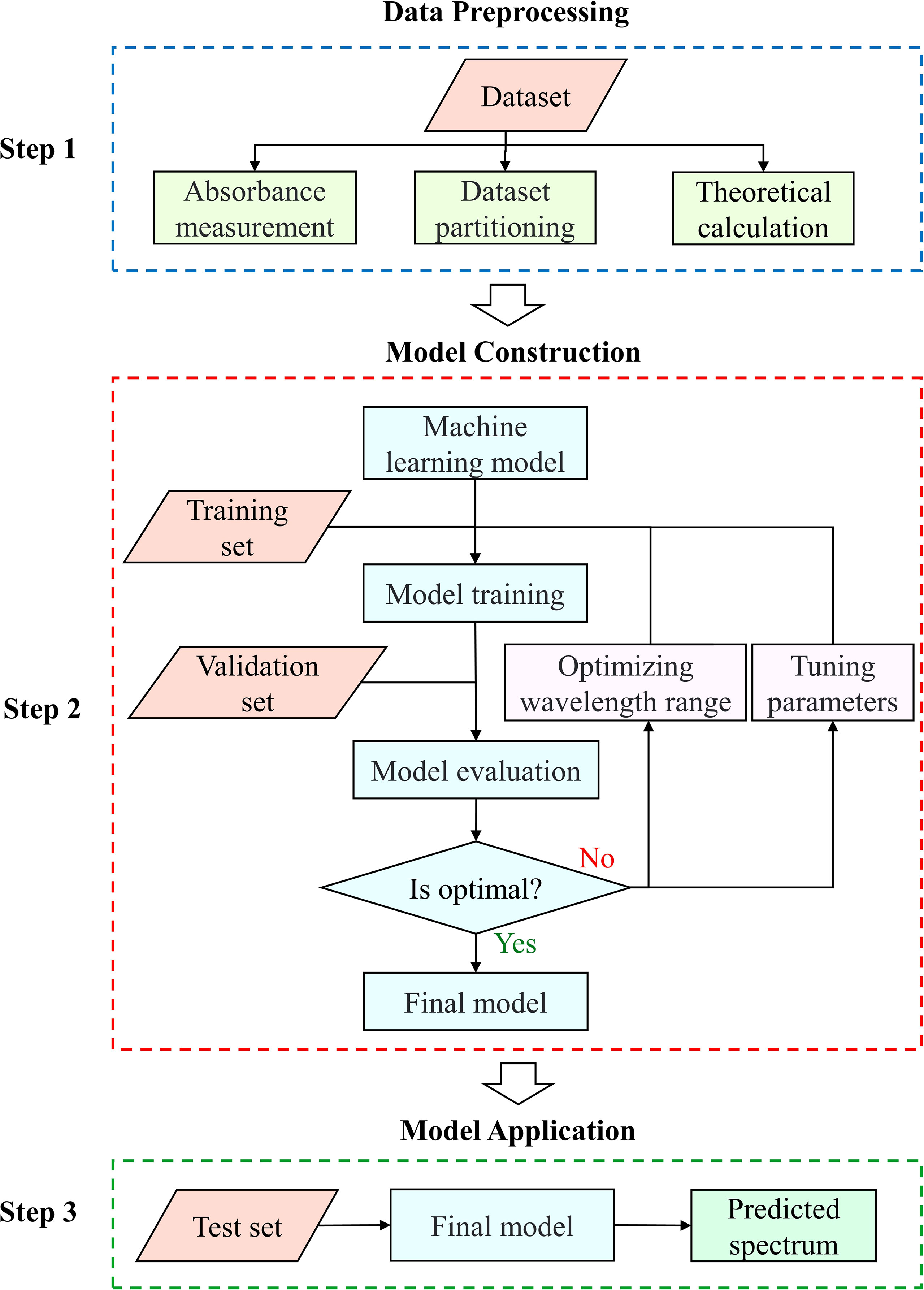
In this study, the BPNN, RF and XGBoost algorithms were used to establish the spectral prediction model of CDOM, respectively. The flow chart of the model development is shown in Figure 2, which includes three steps.
Step 1. Data preprocessing. Use the instruments and methods mentioned above to obtain the raw seawater spectra of each sample. Analyze the and concentrations in the samples using colorimetric Griess assay. Then, the theoretical CDOM spectra were calculated using Equation (3).
Step 2. Model construction. In order to avoid overfitting, five-fold cross validation was used to select the optimal model parameters. The absorption spectra of the samples in the training set were used to train the three machine learning models, respectively, and then the validation set samples were evaluated with the evaluation metrics in Section 2.4. In order to obtain the best prediction results, the input wavelength range and model parameters (layers, the node number and training epochs of BPNN, the number of trees of RF and XGBoost, etc.) need to be tuned according to the evaluation results.
Step 3. Model application. Use the built BPNN, RF and XGBoost models to predict the CDOM absorption spectra between 215 and 350 nm for the samples in the test set. The prediction results were evaluated by comparing to the theoretical spectra obtained in Step 1.
3 Results and discussion
3.1 The theoretic CDOM absorption spectra
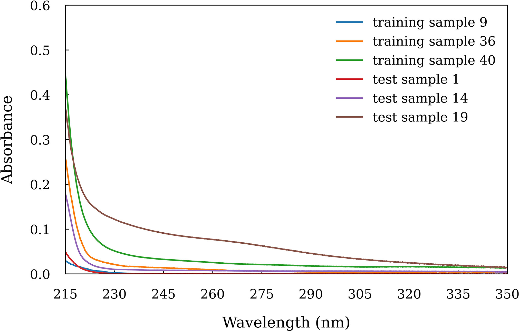
The absorption spectra of CDOM between 215 and 350 nm in each sample was calculated based on Equation (3). The absorbance below 215 nm was not calculated because the absorbance was saturate. The results show that all the spectra show a similarly exponential decay model, with the absorbance decreasing rapidly from 215 and 240 nm and then decreasing slowly above 240 nm. Comparatively, the coastal water samples with lower salinity had higher absorbance of CDOM. For example, the train sample 40 (salinity = 15.54) and test sample 19 (salinity = 11.58) had absorbance of higher than 0.35 at 215 nm (Figure 3). While those samples with higher salinity had lower absorbance, such as the train sample 9 (salinity = 33.23) and test sample 1 (salinity = 31.44) (Figure 3).
The presence of a broad spectral peak between 260 and 275 nm characterized most samples, which had also been found in previous studies (Guenther et al., 2001; Johnson and Coletti, 2002). The reason was ascribed to the specific kind of organic matter. Noteworthy, the sulfides have also an absorbance peak near 260 nm. An absorbance of > 0.5 has been observed in sediment pore water (Guenther et al., 2001). However, in oxygenated and alkaline seawater, the sulfide concentrations are normally very low. Its absorbance can be neglected.
3.2 Selection of wavelength range for model input
The wavelength selection is to choose an optimal wavelength range of raw seawater spectra with which the established model has the best prediction ability. Contrarily, the inclusion of uninformative wavelengths in the training process would affect the accuracy of prediction and model interpretability. Here, we trained the models using the raw seawater absorption spectra with different wavelength ranges between 215 and 350 nm, e.g. 230-350, 240-350, 230-340, 240-340, 250-350 nm, etc. Then, the results were evaluated by calculating the R2, MAE and RMSE between the predicted CDOM spectra and theoretical CDOM spectra of the validation set. The wavelength interval with maximal R2 and minimal MAE and RMSE was selected as the optimal wavelength range. The prediction accuracies of the models using different wavelength ranges are shown in Figure 4. The results suggest that the optimal wavelength range was 250-350 nm for both the BPNN and XGBoost models, which had the maximal R2 of 0.786 and 0.809, the minimal RMSE of 0.0103 and 0.0095 and the minimal MAE of 0.0043 and 0.0037 respectively. For the RF model, although 240-350 nm was the optimal wavelength interval, its prediction results (R2 = 0.8061, RMSE = 0.0096, MAE = 0.0036) were very close to that of 250-350 nm range (R2 = 0.8040, RMSE = 0.0095, MAE = 0.0037). Hence, 250-350 nm was chosen to train the three models and predict the CDOM spectra between 215 and 350 nm.
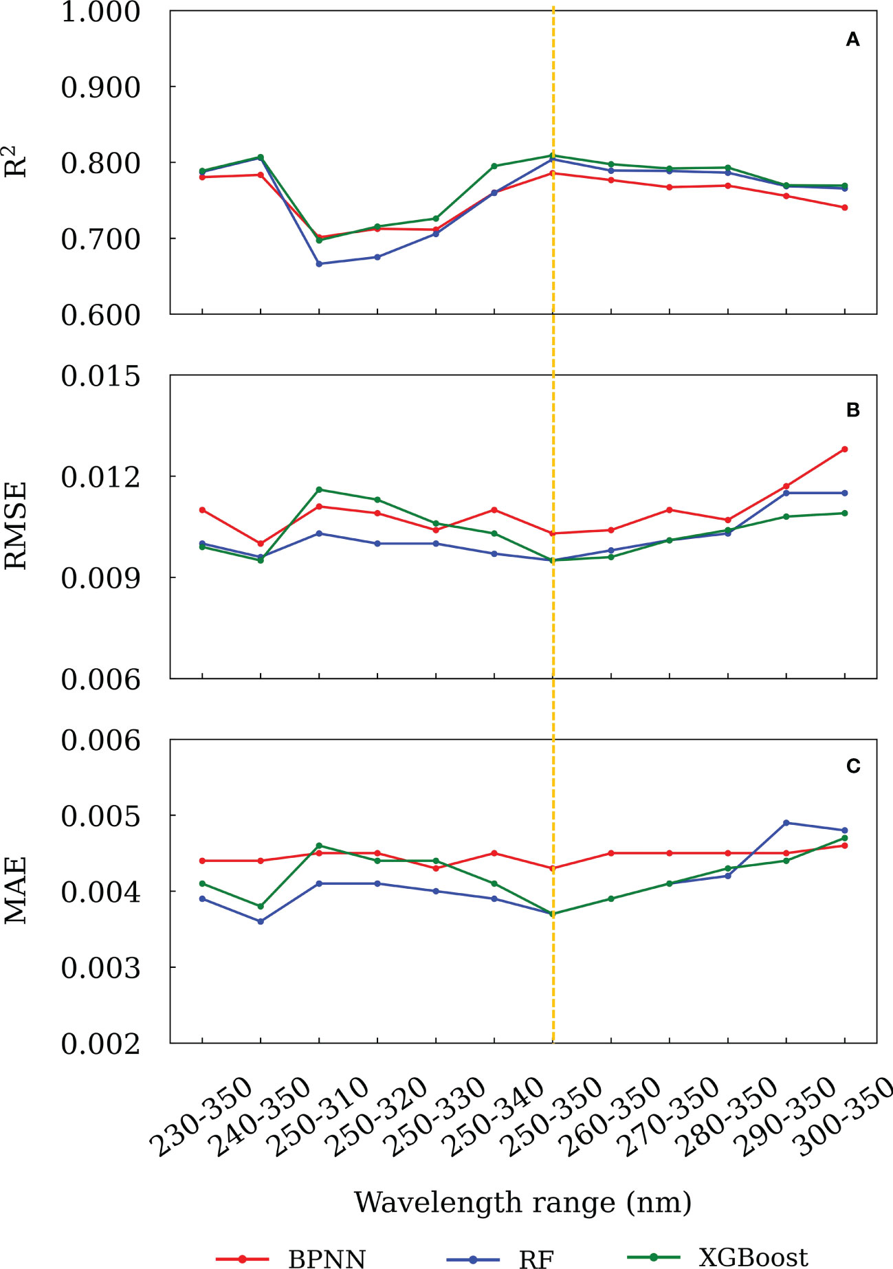
Figure 4 The (A) R2, (B) RMSE and (C) MAE between the predicted and theoretical absorbance for different wavelength ranges.
3.3 Optimization of model parameters
3.3.1 The epoch of the BPNN model
In this study, the BPNN model consisted of three FC layers with nonlinear activation functions. The first two activation functions were the ReLU functions, while the third activation function was the Sigmoid function. The number of training epoch is another important model parameter for BPNN model. The inadequate or excessive training epochs may cause underfitting or overfitting and affect the prediction performance. The R2 and RMSE of the validation set were used to determine the optimal number of training epoch for the model. The BPNN model was trained 1000 epochs using samples of the training set, and the resultant R2 and RMSE of the training and validation sets are shown in Figure 5A, B. It suggests that the R2 of both the training and validation sets increased as the epoch increased and remained stable until 200 epochs (Figure 5A). Accordingly, the RMSE decreased with the increase of epoch till 200 (Figure 5B). Therefore, 200 epochs were selected as the training times for the BPNN model.
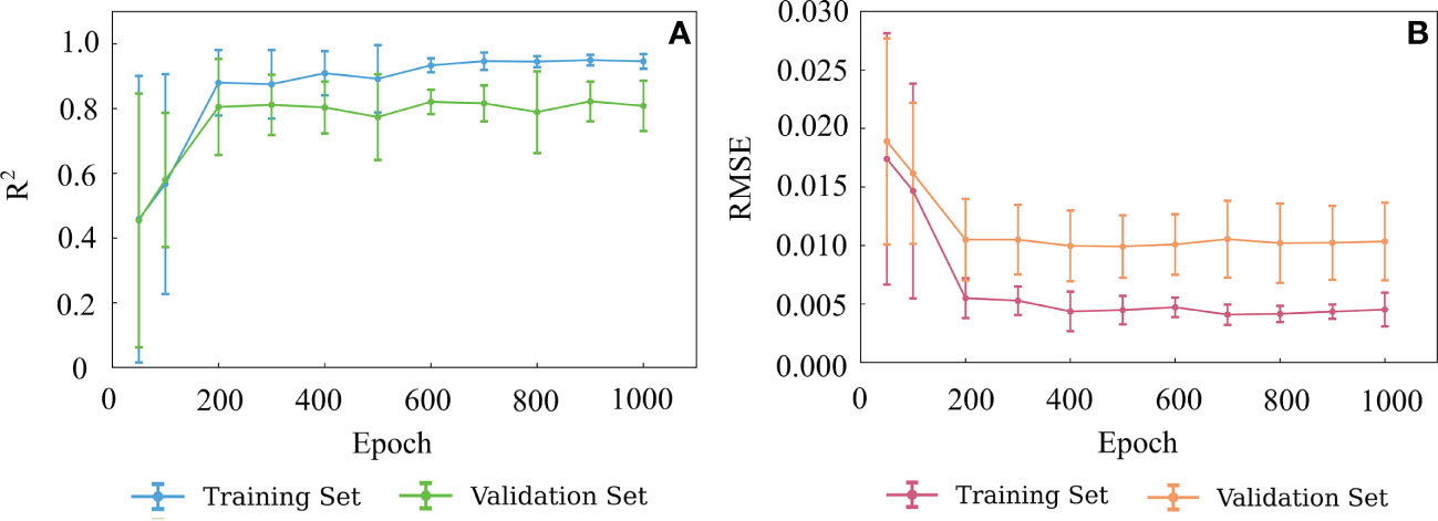
Figure 5 Variation of R2 (A) and RMSE (B) with the numbers of epoch of the BPNN model. The error bars indicate ± 1 standard deviation.
3.3.2 The number of decision trees of the RF and XGBoost model
In XGBoost and Random Forest models, the number of trees represent the number of base classifiers. Less trees would lead to a poor model performance and higher prediction error. Since XGBoost and RF models don’t cause over-fitting, the number of trees can be as large as possible to make the model have good generalization ability. However, the superfluous trees would increase the complexity of the model and the running time of the model.
Similar to BPNN, the R2 and RMSE of the training and validation sets were applied to determine the optimal numbers of trees for XGBoost and RF models, which are shown in Figures 6A-D. For XGBoost model, as the tree numbers were more than 200, the R2 was the largest and RMSE was the lowest for both the training and validation sets. Hence, 200 was chosen as the optimal number of trees. Similarly, for RF model, 50 was chosen as the optimal number of trees.
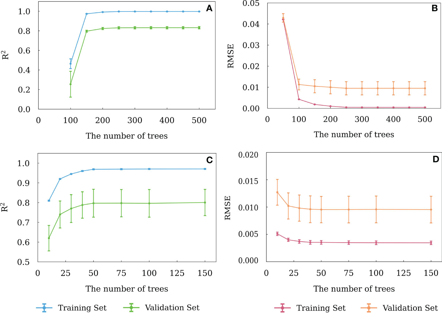
Figure 6 Variation of R2 and RMSE of the RF (A, B) and XGBoost (C, D) models with different numbers of decision trees. The error bars indicate ± 1 standard deviation.
3.4 Comparison of the results from the built BPNN, RF and XGBoost models
Based on the optimal wavelength range and model parameters, the three machine learning models were trained using the spectra of the training set samples. Then it was used to predict the CDOM spectra of the test set samples. In Figure 7, we show the prediction results of CDOM spectra of several samples in the test set. For comparison, the theoretical CDOM spectral are also shown. The results suggest that there was no significant difference between the results from the three models, and they were consistent with the theoretical CDOM spectra between 215-350 nm. Comparatively, the XGBoost model gave the best prediction results, which had the highest R2 and lowest RMSE and MAE (Figure 4).
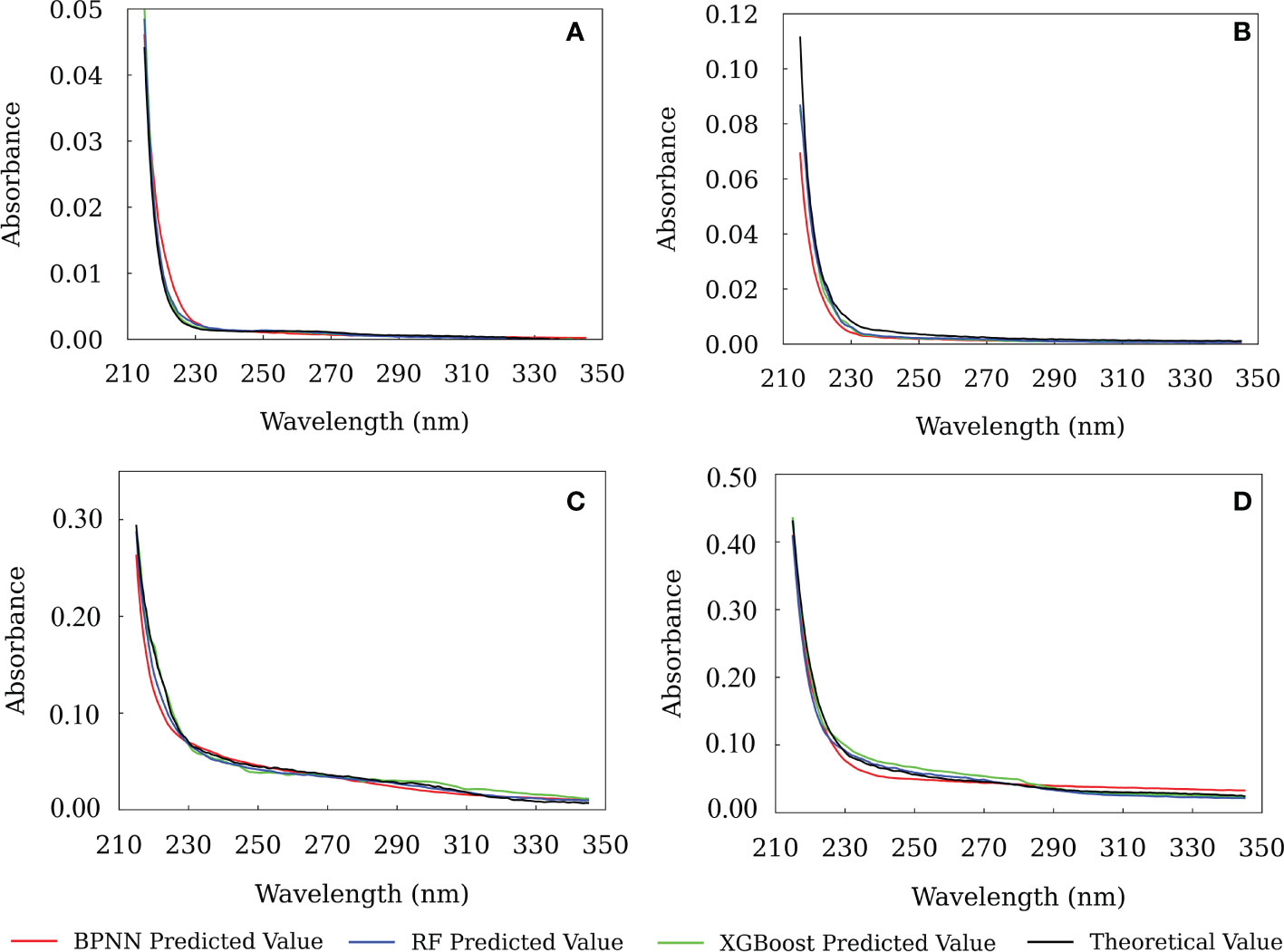
Figure 7 The predicted results from the BPNN, RF and XGBoost models. (A) - test sample 4, (B) - test sample 16, (C) - test sample 20, (D) - test sample 8.
Furthermore, we plotted the predicted absorbance at 215, 220 and 240 nm of all the samples in the test set against the theoretical absorbance in Figure 8. The correlation coefficients (R2) and slopes can be used to evaluate the correlation and close proximity between the predicted and theoretical absorbance. We found that both XGBoost and RF models have better R2 and slope at 215, 220 and 240 nm. While XGBoost model had slopes closer to 1 (0.92, 0.92 and 1.00), although they had similar R2 values. This indicates the predicted absorbance was more fit to the theoretical value. It is known that, as integrated learning algorithms, XGBoost and RF can overcome the disadvantage of overfitting by creating multiple decision trees (Breiman, 2001; Chen and Guestrin, 2016). In addition, both XGBoost and RF have been shown to outperform BPNN in prediction performance for training set with small sample size (Luckner et al., 2017; Ogunleye and Wang, 2019; Han et al., 2021). However, the difference between RF and XGBoost is that the RF algorithm focuses on the final voting results of all decision trees and can only reduce the variance, while the XGBoost algorithm focuses on the residuals generated by the last iteration. Therefore, XGBoost can reduce both variance and bias (Oh and Lee, 2017; Zhang et al., 2019). These reasons might explain the best performance for XGBoost model, especially for the data sets with limited samples.
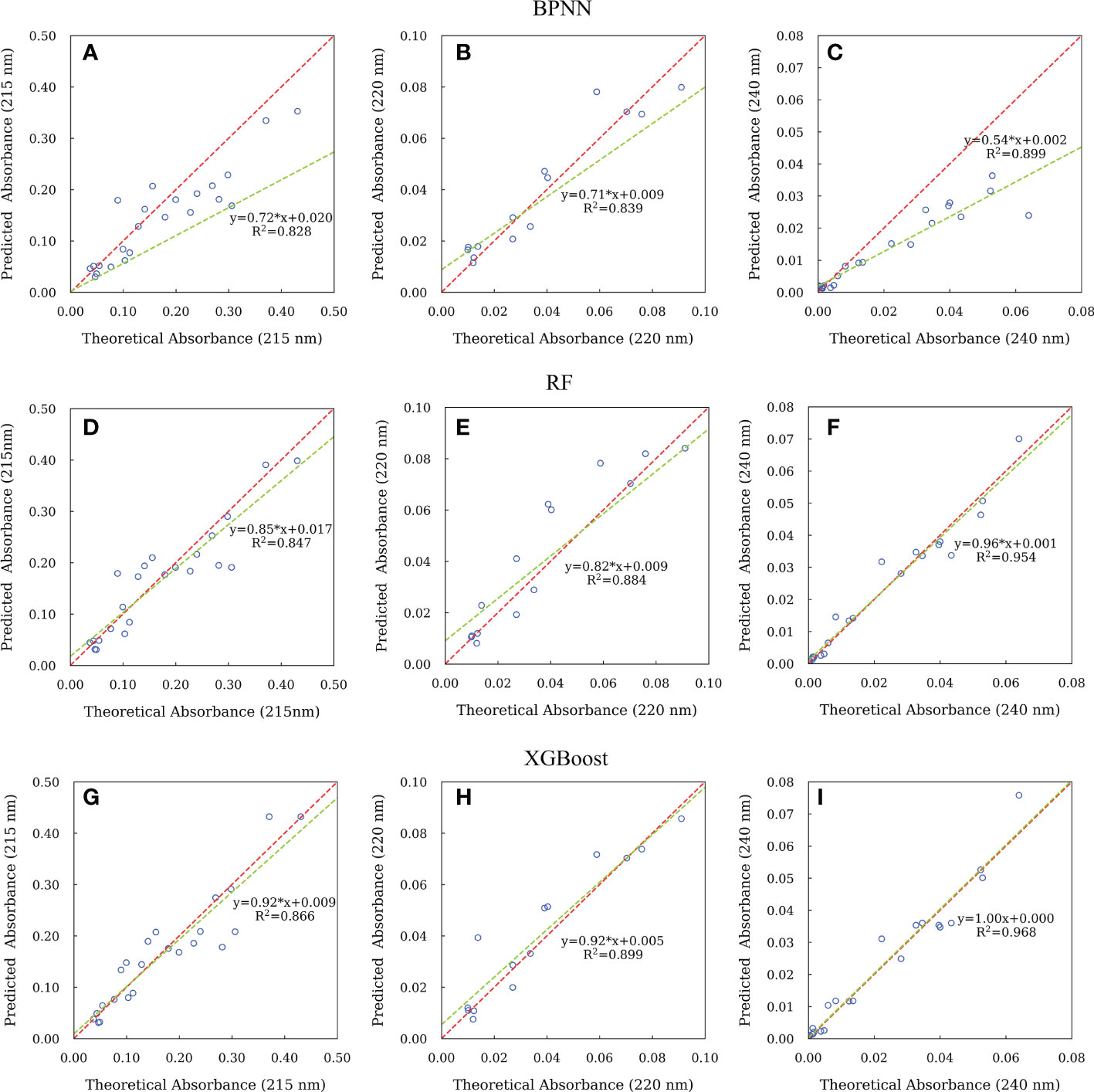
Figure 8 The relationships between the predicted and theoretical absorbance of CDOM at 215, 220 and 240 nm for samples in the test set using BPNN (A-C), RF (D-F) and XGBoost (G-I) algorithms. Red dash lines represent line of 1:1 of predicted to theoretical absorbance. Green solid lines represent fitted line between the predicted and theoretical absorbance.
It should be noted that the build method can also be used to predict the UV absorption spectra for seawater samples collected from a variety of marine environments, such as eutrophic or oligotrophic waters. However, we recommend using local training sets, considering that the CDOM compositions and light absorbance might vary in different waters.
3.5 The spectra slopes of short wavelengths
It is known that spectra slope, S in Equation (1), is an important parameter to describe the shape of UV-Vis spectra, which can be used as indicators of molecular size and weight and its sources (Bricaud et al., 1981; Helms et al., 2008; Stedmon and Nelson, 2015). For absorption measurements of CDOM, the main problem is the low absorption at long wavelengths in combination with the limited length of the cuvette and the possible scattering effect of particles and bubbles. The slope of the shorter wavelengths can be measured with high precision and therefore more reliable than the values at longer wavelengths (Markager and Vincent, 2000; Helms et al., 2008). However, the calculation of S values at shorter wavelength than 240 nm based on the raw spectra is problematic due to the interference of other substances besides CDOM.
Generally, the widely used spectra slope is calculated between 275 and 295 nm by traditional method (S275-295T), which is based on the raw spectra and employing non-linear regression of Equation (1). For comparison, we use our predicted spectra by XGBoost algorithm to obtain the spectra slopes of the test set samples between 215 and 240 nm (S215-240) and between 215 and 275 nm (S215-275). The reference wavelength was set at 295 nm. The results are shown in Table 2. It suggests that S215-240 and S215-275 have similar values ranging from 0.030 to 0.066 nm-1 and 0.024 to 0.044 nm-1, respectively, which are almost twice the S275-295T (0.015 to 0.035 nm-1). This result is consistent with previous observations indicating increasing S values with decreasing wavelengths (Twardowski et al., 2004; Swan et al., 2013; Wei et al., 2016).

Table 2 Comparison of S215-240 and S215-275 based on the predicted spectra and S275-295T calculated using the traditional method.
The relationships between S and salinity are plotted in Figure 9. We found that all the S values show similar distribution shape. For nearshore samples with lower salinities (<27), there is no big difference in S, suggesting that these samples have similar CDOM composition. However, for marine samples with comparatively higher salinities (>27), there is an increasing trend of S with increasing salinities. Previous efforts have demonstrated that S correlates strongly with molecular weight and size (Helms et al., 2008; Stedmon and Nelson, 2015). Low molecular weight CDOM has stronger absorbance at shorter wavelengths (<300 nm), causing higher (or steeper) spectra slopes, and vice versa (Stedmon et al., 2000; Helms et al., 2008; Lei et al., 2019). Generally, marine CDOM has chromophores with smaller molecule size and weight, while terrestrially dominated CDOM has higher molecule size and weight (Stedmon et al., 2000; Helms et al., 2008; Fichot and Benner, 2012; Zhao et al., 2021). Consequently, our results support these previous observations. Interestingly, both S215-240 and S215-275 are more relevant with salinities (R2>0.70, Figure 9A, B) than S275-295T (R2 = 0.34, Figure 9C) for marine CDOM, indicating that spectra slopes of shorter wavelengths might be the better proxies for marine CDOM than that of longer wavelengths.
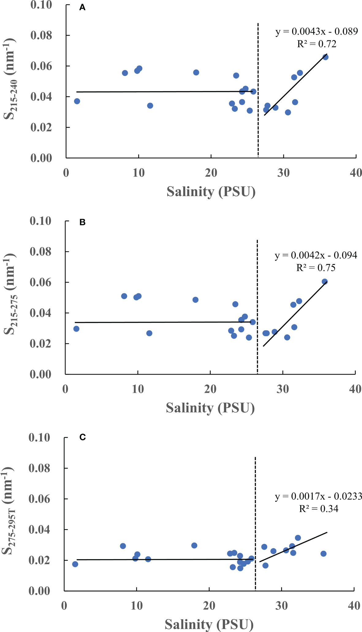
Figure 9 The correlation between salinities and spectra slopes (A)-S215-240, (B)-S215-275, (C)-S275-295T.
4 Conclusions
We present a technique of machine learning to model the UV absorption spectra of CDOM in seawater between 215 and 350 nm for the first time. Three machine learning models, BPNN, RF and XGBoost, were constructed based on the raw seawater UV absorption spectra and the results were compared with each other.
The optimal input wavelength range for the three models was 250-350 nm. By choosing the optimal model parameters based on five-fold cross validation, all the three models can well predict the CDOM absorption spectra between 215 and 350 nm. Comparatively, the XGBoost model had the best prediction performance, which had the highest R2 and lowest RMSE and MAE.
Spectra slopes of short wavelengths, S215-240 and S215-275, are higher than the widely used S275-295T. More interestingly, S215-240 and S215-275 have better correlation with salinity than S275-295T for marine CDOM, suggesting that spectra slopes of short wavelengths might be more suitable to describe marine CDOM. We strongly advocate inclusion of spectra slopes of short wavelength in future CDOM studies.
Data availability statement
The raw data supporting the conclusions of this article will be made available by the authors, without undue reservation.
Author contributions
HW and AJ are the principal investigators and initiated the project. AJ and HW wrote the first draft of the manuscript, paper. AJ and LW performed the spectral measurements. YW contributed to the data analysis and data processing. All authors contributed to the article and approved the submitted version.
Funding
This work was supported by The National Key Research and Development Program of China (No. 2022YFC2805504) and National Natural Science Foundation of China (No. 42076062).
Acknowledgments
The authors would like to thank all the participants and crew of the cruises KECES-2020 for collecting samples.
Conflict of interest
The authors declare that the research was conducted in the absence of any commercial or financial relationships that could be construed as a potential conflict of interest.
Publisher’s note
All claims expressed in this article are solely those of the authors and do not necessarily represent those of their affiliated organizations, or those of the publisher, the editors and the reviewers. Any product that may be evaluated in this article, or claim that may be made by its manufacturer, is not guaranteed or endorsed by the publisher.
References
Abdel-Rahman E. M., Mutanga O., Odindi J., Adam E., Odindo A., Ismail R. (2017). Estimating Swiss chard foliar macro-and micronutrient concentrations under different irrigation water sources using ground-based hyperspectral data and four partial least squares (PLS)-based (PLS1, PLS2, SPLS1 and SPLS2) regression algorithms. Comput. Electron. Agr. 132, 21–33. doi: 10.1016/j.compag.2016.11.008
Armstrong F. A. J. (1963). Determination of nitrate in water ultraviolet spectrophotometry. Anal. Chem. 35, 1292–1294. doi: 10.1021/ac60202a036
Baker A., Spencer R. G. (2004). Characterization of dissolved organic matter from source to sea using fluorescence and absorbance spectroscopy. Sci. Total Environ. 333, 217–232. doi: 10.1016/j.scitotenv.2004.04.013
Bricaud A., Morel A., Prieur L. (1981). Absorption by dissolved organic matter of the sea (yellow substance) in the UV and visible domains. Limnol. Oceanogr. 26, 43–53. doi: 10.4319/lo.1981.26.1.0043
Cao F., Miller W. L. (2015). A new algorithm to retrieve chromophoric dissolved organic matter (CDOM) absorption spectra in the UV from ocean color. J. Geophys. Res. Oceans 120, 496–516. doi: 10.1002/2014JC010241
Chen T., Guestrin C. (2016). “Xgboost: A scalable tree boosting system,” in Proc. 22nd ACM SIGKDD Int. Conf. on Knowledge Discovery and Data Mining. Association for Computing Machinery, New York, NY, USA, 785–794. doi: 10.1145/2939672.2939785
Coble P. G., Lead J., Baker A., Reynolds D. M., Spencer R. G. (2014). Aquatic organic matter fluorescence (Cambridge, MA, USA: Cambridge University Press).
Cutler A., Cutler D. R., Stevens J. R. (2012). “Random forests,” in Ensemble machine learning (Boston, MA, USA: Springer), 157–175. doi: 10.1007/978-1-4419-9326-7_5
Del Castillo C. E., Coble P. G. (2000). Seasonal variability of the colored dissolved organic matter during the 1994–95 NE and SW monsoons in the Arabian Sea. Deep Sea Res. Part II: Topical Stud. Oceanography 47, 1563–1579. doi: 10.1016/S0967-0645(99)00154-X
Dong Y., Fu Z., Peng Y., Zheng Y., Yan H., Li X. (2020). Precision fertilization method of field crops based on the wavelet-BP neural network in China. J. Clean Prod. 246, 118735. doi: 10.1016/j.jclepro.2019.118735
Erb R. J. (1993). Introduction to backpropagation neural network computation. Pharm. Res. 10, 165–170. doi: 10.1023/A:1018966222807
Fan J., Wang X., Wu L., Zhou H., Zhang F., Yu X., et al. (2018). Comparison of support vector machine and extreme gradient boosting for predicting daily global solar radiation using temperature and precipitation in humid subtropical climates: A case study in China. Energ. Convers. Manage. 164, 102–111. doi: 10.1016/j.enconman.2018.02.087
Fichot C. G., Benner R. (2012). The spectral slope coefficient of chromophoric dissolved organic matter (S275–295) as a tracer of terrigenous dissolved organic carbon in river-influenced ocean margins. Limnol. Oceanogr. 57, 1453–1466. doi: 10.4319/lo.2012.57.5.1453
Guenther E. A., Johnson K. S., Coale K. H. (2001). Direct ultraviolet spectrophotometric determination of total sulfide and iodide in natural waters. Anal. Chem. 73, 3481–3487. doi: 10.1021/ac0013812
Guo W., Stedmon C. A., Han Y., Wu F., Yu X., Hu M. (2007). The conservative and non-conservative behavior of chromophoric dissolved organic matter in Chinese estuarine waters. Mar. Chem. 107, 357–366. doi: 10.1016/j.marchem.2007.03.006
Han S., Williamson B. D., Fong Y. (2021). Improving random forest predictions in small datasets from two-phase sampling designs. BMC Med. Inform. Decis. 21, 1–9. doi: 10.1186/s12911-021-01688-3
Hecht-Nielsen R. (1992). Theory of the backpropagation neural network. neural networks for perception. Neural Networks for Percept. 2 computation, learning, architectures, Harcourt Brace & Co., USA, 65–93. doi: 10.1016/B978-0-12-741252-8.50010-8
Helms J. R., Stubbins A., Ritchie J. D., Minor E. C., Kieber D. J., Mopper K. (2008). Absorption spectral slopes and slope ratios as indicators of molecular weight, source, and photobleaching of chromophoric dissolved organic matter. Limnol. Oceanogr. 53, 955–969. doi: 10.4319/lo.2008.53.3.0955
Jørgensen L., Markager S., Maar M. (2014). On the importance of quantifying bioavailable nitrogen instead of total nitrogen. Biogeochemistry 117, 455–472. doi: 10.1007/s10533-013-9890-9
Johnson K. S., Coletti L. J. (2002). In situ ultraviolet spectrophotometry for high resolution and long-term monitoring of nitrate, bromide and bisulfide in the ocean. Deep Sea Res. Part I.: Oceanographic Res. Papers. 49, 1291–1305. doi: 10.1016/S0967-0637(02)00020-1
Khoshgoftaar T. M., Golawala M., Van Hulse J. (2007). “An empirical study of learning from imbalanced data using random forest,” in 19th IEEE International Conference on Tools with Artificial Intelligence (ICTAI 2007), Vol. 2 (IEEE), Patras, Greece 2007, 310–317. doi: 10.1109/ICTAI.2007.49
Lei X., Pan J., Devlin A. (2019). Characteristics of absorption spectra of chromophoric dissolved organic matter in the pearl river estuary in spring. Remote Sens. 11 (13), 1533. doi: 10.3390/rs11131533
Li J., Cheng J., Shi J., Huang F. (2012). Brief introduction of back propagation (BP) neural network algorithm and its improvement (Berlin Heidelberg: Springer), 553–558. doi: 10.1007/978-3-642-30223-7_87
Li P., Hur J. (2017). Utilization of UV-vis spectroscopy and related data analyses for dissolved organic matter (DOM) studies: A review. Crit. Rev. Env. Sci. Tec. 47, 131–154. doi: 10.1080/10643389.2017.1309186
Luckner M., Topolski B., Mazurek M. (2017). “Application of XGBoost algorithm in fingerprinting localisation task,” in IFIP International Conference on Computer Information Systems and Industrial Management (Cham, Switzerland: Springer). doi: 10.1007/978-3-319-59105-6_57
Marín-García M., Tauler R. (2020). Chemometrics characterization of the llobregat river dissolved organic matter. Chemometr. Intell. Lab. 201, 104018. doi: 10.1016/j.chemolab.2020.104018
Markager S., Vincent W. F. (2000). Spectral light attenuation and the absorption of UV and blue light in natural waters. Limnol. Oceanogr. 45 (3), 642–650. doi: 10.4319/lo.2000.45.3.0642
Massicotte P., Markager S. (2016). Using a Gaussian decomposition approach to model absorption spectra of chromophoric dissolved organic matter. Mar. Chem. 180, 24–32. doi: 10.1016/j.marchem.2016.01.008
McKnight D. M., Boyer E. W., Westerhoff P. K., Doran P. T., Kulbe T., Andersen D. T. (2001). Spectrofluorometric characterization of dissolved organic matter for indication of precursor organic material and aromaticity. Limnol. Oceanogr. 46, 38–48. doi: 10.4319/lo.2001.46.1.0038
Murphy K. R., Stedmon C. A., Waite T. D., Ruiz G. M. (2008). Distinguishing between terrestrial and autochthonous organic matter sources in marine environments using fluorescence spectroscopy. Mar. Chem. 108, 40–58. doi: 10.1016/j.marchem.2007.10.003
Murphy K., Timko S. A., Gonsior M., Powers L., Wünsch U., Stedmon C. A. (2018). Photochemistry illuminates ubiquitous organic matter fluorescence spectra. Environ. Sci. Technol. 52, 11243–11250. doi: 10.1021/acs.est.8b02648
Nelson N. B., Gauglitz J. M. (2016). Optical signatures of dissolved organic matter transformation in the global ocean. Front. Mar. Sci. 2. doi: 10.3389/fmars.2015.00118
Nelson N. B., Siegel D. A. (2013). The global distribution and dynamics of chromophoric dissolved organic matter. Annu. Rev. Mar. Sci. 5, 447–476. doi: 10.1146/annurev-marine-120710-100751
Nima C., Frette Ø., Hamre B., Stamnes J. J., Chen Y. C., Sørensen K., et al. (2019). CDOM absorption properties of natural water bodies along extreme environmental gradients. Water 11, 1988. doi: 10.3390/w11101988
Ogunleye A., Wang Q. G. (2019). XGBoost model for chronic kidney disease diagnosis. IEEE ACM T. Comput. Bi. 17, 2131–2140. doi: 10.1109/TCBB.2019.2911071
Oh H. J., Lee S. (2017). Shallow landslide susceptibility modeling using the data mining models artificial neural network and boosted tree. Appl. Sci. 7, 1000. doi: 10.3390/app7101000
Primadusi U., Cahyadi A. I., Prasetyo D., Wahyunggoro O. (2016). “Backpropagation neural network models for LiFePO4 battery,” in Advances of Science and Technology for Society: Proceedings of the 1st International Conference on Science and Technology, Vol. 1755 (New York, USA: AIP Publishing LLC). doi: 10.1063/1.4958527
Quinonero-Candela J., Sugiyama M., Schwaighofer A., Lawrence N. D. (2008). Dataset shift in machine learning (Cambridge, MA, USA: Mit Press).
Ruescas A. B., Hieronymi M., Mateo-Garcia G., Koponen S., Kallio K., Camps-Valls G. (2018). Machine learning regression approaches for colored dissolved organic matter (CDOM) retrieval with S2-MSI and S3-OLCI simulated data. Remote Sens. 10, 786. doi: 10.3390/rs10050786
Rumelhart D. E., McClelland J. L. (1986). PDP Models and general issues in cognitive science. parallel distributed processing: Explorations in the microstructure of cognition Vol. 1 (Cambridge, MA, USA: Foundations (Mit Press)), 110–146. doi: 10.5555/104279.104288
Sakamoto C. M., Johnson K. S., Coletti L. J. (2009). Improved algorithm for the computation of nitrate concentrations in seawater using an in situ ultraviolet spectrophotometer. Limnol. Oceanogr.: Methods 7, 132–143. doi: 10.4319/lom.2009.7.132
Stedmon C. A., Bro R. (2008). Characterizing dissolved organic matter fluorescence with parallel factor analysis: A tutorial. Limnol. Oceanogr. Meth. 6, 572–579. doi: 10.4319/lom.2008.6.572
Stedmon C. A., Markager S. (2001). The optics of chromophoric dissolved organic matter (CDOM) in the Greenland Sea: An algorithm for differentiation between marine and terrestrially derived organic matter. Limnol. Oceanogr. 46, 2087–2093. doi: 10.4319/lo.2001.46.8.2087
Stedmon C. A., Markager S., Bro R. (2003). Tracing dissolved organic matter in aquatic environments using a new approach to fluorescence spectroscopy. Mar. Chem. 82, 239–254. doi: 10.1016/S0304-4203(03)00072-0
Stedmon C. A., Markager S., Kaas H. (2000). Optical properties and signatures of chro-mophoric dissolved organic matter (CDOM) in Danish coastal waters. Estuar. Coast. Shelf Sci. 51 (2), 267–278. doi: 10.1006/ecss.2000.0645
Stedmon C. A., Nelson N. B. (2015). Biogeochemistry of marine dissolved organic matter. Eds. Hansell D. A., Carlson C. A. (Boston: Academic Press), 481–508.
Sun X., Li P., Zhou Y., He C., Cao F., Wang Y., et al. (2022). Linkages between optical and molecular signatures of dissolved organic matter along the Yangtze river estuary to East China Sea continuum. Front. Mar. Sci. 9. doi: 10.3389/fmars.2022.933561
Swan C. M., Nelson N. B., Siegel D. A., Fields E. A. (2013). A model for remote estimation of ultraviolet absorption by chromophoric dissolved organic matter based on the global distribution of spectral slope. Remote Sens. Environ. 136, 277–285. doi: 10.1016/j.rse.2013.05.009
Tawfik M. E., Bishay P. L., Sadek E. A. (2018). Neural network-based second order reliability method (NNBSORM) for laminated composite plates in free vibration. Comp. Model. Eng. 115, 105–129. doi: 10.3970/cmes.2018.115.105
Twardowski M. S., Boss E., Sullivan J. M., Donaghay P. L. (2004). Modeling the spectral shape of absorption by chromophoric dissolved organic matter. Mar. Chem. 89, 69–88. doi: 10.1016/j.marchem.2004.02.008
Verrelst J., Muñoz J., Alonso L., Delegido J., Rivera J. P., Camps-Valls G., et al. (2012). Machine learning regression algorithms for biophysical parameter retrieval: Opportunities for sentinel-2 and-3. Remote Sens. Environ. 118, 127–139. doi: 10.1016/j.rse.2011.11.002
Wei J., Lee Z., Ondrusek M., Mannino A., Tzortziou M., Armstrong R. (2016). Spectral slopes of the absorption coefficient of colored dissolved and detrital material inverted from UV-visible remote sensing reflectance. J. Geophys. Res. Oceans 121, 1953–1969. doi: 10.1002/2015JC011415
Whitehead R. F., De Mora S., Demers S., Gosselin M., Monfort P., Mostajir B. (2000). Interactions of ultraviolet-b radiation, mixing, and biological activity on photobleaching of natural chromophoric dissolved organic matter: A mesocosm study. Limnol. Oceanogr. 45, 278–291. doi: 10.4319/lo.2000.45.2.0278
Yamashita Y., Boyer J. N., Jaffé R. (2013). Evaluating the distribution of terrestrial dissolved organic matter in a complex coastal ecosystem using fluorescence spectroscopy. Cont. Shelf Res. 66, 136–144. doi: 10.1016/j.csr.2013.06.010
Yang L., Guo W., Hong H., Wang G. (2013). Non-conservative behaviors of chromophoric dissolved organic matter in a turbid estuary: Roles of multiple biogeochemical processes. Estuar. Coast. Shelf S. 133, 285–292. doi: 10.1016/j.ecss.2013.09.007
Zhang Y., Ge T., Tian W., Liou Y. A. (2019). Debris flow susceptibility mapping using machine-learning techniques in shigatse area, China. Remote Sens. 11, 2801. doi: 10.3390/rs11232801
Zhang Y., Zhou L., Zhou Y., Zhang L., Yao X., Shi K., et al. (2021). Chromophoric dissolved organic matter in inland waters: Present knowledge and future challenges. Sci. Total Environ. 759, 143550. doi: 10.1016/j.scitotenv.2020.143550
Zhao J., Cao W., Xu Z., Ai B., Yang Y., Jin G., et al. (2018). Estimating CDOM concentration in highly turbid estuarine coastal waters. J. Geophys. Res.-Oceans. 123, 5856–5873. doi: 10.1029/2018JC013756
Zhao L., Gao L., Guo L. (2021). Seasonal variations in molecular size of chromophoric dissolved organic matter from the lower changjiang (Yangtze) river. J. Geophys. Res. 126, e2020JG006160. doi: 10.1029/2020JG006160
Keywords: chromophoric dissolved organic matter, machine learning algorithm, back propagation neural network, random forest, extreme gradient boosting
Citation: Ju A, Wang H, Wang L and Weng Y (2023) Application of machine learning algorithms for prediction of ultraviolet absorption spectra of chromophoric dissolved organic matter (CDOM) in seawater. Front. Mar. Sci. 10:1065123. doi: 10.3389/fmars.2023.1065123
Received: 09 October 2022; Accepted: 16 January 2023;
Published: 30 January 2023.
Edited by:
David C. Podgorski, University of New Orleans, United StatesCopyright © 2023 Ju, Wang, Wang and Weng. This is an open-access article distributed under the terms of the Creative Commons Attribution License (CC BY). The use, distribution or reproduction in other forums is permitted, provided the original author(s) and the copyright owner(s) are credited and that the original publication in this journal is cited, in accordance with accepted academic practice. No use, distribution or reproduction is permitted which does not comply with these terms.
*Correspondence: Hu Wang, d2FuZ2h1QHRvbmdqaS5lZHUuY24=
 Aobo Ju
 Hu Wang
 Lequan Wang