Filling Gaps in Trawl Surveys at Sea through Spatiotemporal and Environmental Modelling

International scientific fishery survey programmes systematically collect samples of target stocks’ biomass and abundance and use them as the basis to estimate stock status in the framework of stock assessment models. The research surveys can also inform decision makers about Essential Fish Habitat conservation and help define harvest control rules based on direct observation of biomass at the sea. However, missed survey locations over the survey years are common in long-term programme data. Currently, modelling approaches to filling gaps in spatiotemporal survey data range from quickly applicable solutions to complex modelling. Most models require setting prior statistical assumptions on spatial distributions, assuming short-term temporal dependency between the data, and scarcely considering the environmental aspects that might have influenced stock presence in the missed locations. This paper proposes a statistical and machine learning based model to fill spatiotemporal gaps in survey data and produce robust estimates for stock assessment experts, decision makers, and regional fisheries management organizations. We apply our model to the SoleMon survey data in North-Central Adriatic Sea (Mediterranean Sea) for 4 stocks: Sepia officinalis, Solea solea, Squilla mantis, and Pecten jacobaeus. We reconstruct the biomass-index (i.e., biomass over the swept area) of 10 locations missed in 2020 (out of the 67 planned) because of several factors, including COVID-19 pandemic related restrictions. We evaluate model performance on 2019 data with respect to an alternative index that assumes biomass proportion consistency over time. Our model’s novelty is that it combines three complementary components. A spatial component estimates stock biomass-index in the missed locations in one year, given the surveyed location’s biomass-index distribution in the same year. A temporal component forecasts, for each missed survey location, biomass-index given the data history of that haul. An environmental component estimates a biomass-index weighting factor based on the environmental suitability of the haul area to species presence. Combining these components allows understanding the interplay between environmental-change drivers, stock presence, and fisheries. Our model formulation is general enough to be applied to other survey data with lower spatial homogeneity and more temporal gaps than the SoleMon dataset.

1 Introduction

Understanding and estimating the status of fish stocks residing in a marine area, requires continuously collecting stock biomass and abundance samples through scientific surveys. After processing these data, scientific advice can be produced for policymakers to assess the stocks’ status and prevent their depletion. Since 2000, European Member States have been collecting fisheries data in a structured way within the Data Collection Framework (DCF) multi-annual programme (JRC, 2021), and more recently under the EU-MAP programme (EUR-Lex, 2021). They advise for the EU Common Fisheries Policy (CFP) (Frost and Andersen, 2006), collect data according to national work plans, and report the results annually. In the Mediterranean context, the data are eventually analysed by fishery experts of European Regional Fisheries Management Organisations (RFMOs), such as the EU Scientific, Technical and Economic Committee for Fisheries (STECF), and the General Fisheries Commitee for the Mediterranean Sea (GFCM). The resulting recommendations are used in the CFP decision-making processes to regulate fishing activity, monitor Essential Fish Habitat conservation, and predict future resource exploitation scenarios (Rosenberg et al., 2000; Hilborn and Walters, 2013; Froese et al., 2017). The data collected within the DCF are integral to several societal challenges of the EU Programmes and the European Marine Strategy Framework Directive (MSFD) (Long, 2011). In this context, fishery-independent data can come with gaps that must be filled to improve quality and reliability. For example, biomass measurements collected through trawl surveys, across several hauls in a marine area, might miss data for some locations in specific years. These data gaps also affect the estimation of catchability during the survey - a measure of fishery efficiency - which requires that the survey protocol and locations remain constant over the years (Swain et al., 2000; Aeberhard et al., 2018). Other drivers of data biases are the possible non-uniform spatial and temporal sampling and the change of the measurement tools. Various uncontrollable causes contribute to these drivers, such as funding delays, vessel unavailability or damage, long bureaucracy, adverse weather and sea conditions, and lastly, the COVID-19 pandemic (Coro et al., 2022b).

Producing accurate and unbiased spatial time series for fishery-independent surveys is crucial to inform stock assessment models and produce valuable results for decision-makers (Maunder, 2001; Coro, 2020b). However, filling the data with stock biomass estimates requires modelling complex and complementary aspects such as (i) the spatial biomass distribution in the surveyed hauls, (ii) the historical stock presence and biomass in the unsurveyed hauls, and (iii) the environmental conditions that may have favoured or penalised the stock presence in the unsurveyed hauls (Jouffre et al., 2010). Artificial Intelligence, and in particular machine learning, can help model these factors and produce valuable estimates with measured uncertainty.

One of the most commonly used models for geospatial time series reconstruction is the Vector Autoregressive Spatio-Temporal (VAST) model (Thorson and Kristensen, 2016; Thorson, 2019). VAST combines two estimators of average density variation in space and time, modelled as two linear predictors. One predictor approximates the probability of encountering the analysed species in an unsurveyed haul, and the other approximates the expected catch rate. VAST combines these two predictors to estimate stock biomass density in the unsurveyed hauls of a specific survey year. Despite the valuable results this technique can produce (Eisner et al., 2020), it is potentially limited by (i) the exclusion of an explicit modelling of environmental aspects, (ii) the fixed prior assumptions on the predictors’ shapes, and (iii) the linear approximations used. Other studies have applied statistical approaches to infer stock structure (i.e., stock abundance-at-length) from incomplete survey data. In Breivik et al. (2021), a model predicts the number of fishes per year and length class in the unsurveyed hauls. It uses a linear combination of multi-variate Gaussian functions dependent on time, location, and length class. The model assumes that each spatial distribution depends only on the previous year’s distribution. The potential limitations of this modelling approach are (i) the high computational complexity to optimise the multi-variate Gaussian functions, (ii) the weak temporal dependency assumed between the spatial distributions (i.e., one year instead of long-term), and (iii) the ambitious goal to infer the full stock structure from scattered and fragmented spatiotemporal data. Other similar modelling approaches have addressed the same goal using a more complex multi-variate function modelling. For example, state-space statistical models have been used to model biomass alongside recruitment, mortality, and growth (Payne, 2010; Aeberhard et al., 2018). These models infer the principal statistical moments of their target distributions through iterative sampling (Fournier et al., 2012; Coro, 2013), but still assume a one-year time dependency between the samples. Other studies have explored - especially through machine learning modelling - long-term dependencies in non-stationary geospatial time series to predict species presence and temporal persistence, and infer species abundance (Paradinas et al., 2020; Lou et al., 2021). Several other modelling approaches assume that the ratio between the stock biomass (or abundance) in a specific haul and the total biomass remains averagely constant in the survey years. The generated biomass indexes (hereafter named equiproportional) are easily implementable and applicable to heterogeneous survey data. They have been used to fill gaps in the Arctic, North Sea, Norwegian Sea, and the Barents Sea surveys (Schmidt et al., 2009; ICES, 2020; Bergenius et al., 2021). Some studies have tried to enhance these approaches by better modelling the co-variation between the missed hauls and known hauls over the years (Gröger et al., 2001). Although these methodologies are widely used, they are more suited for short time series with few gaps where their basic assumptions are approximately valid.

This paper proposes a new model - made up of three machine learning and statistical sub-models - to fill gaps in the geospatial time series of stock biomass indexes collected by the SoleMon fishery-independent surveys in 2020 (Grati et al., 2013; Scarcella, 2018). SoleMon is an experimental trawl survey collecting fishery-independent data since 2005 to facilitate the sustainable management of fisheries-exploited resources in the North and Central Adriatic Sea, i.e., the GFCM Geographical Sub Area (GSA) 17 (FAO, 1999) (Figure 1). The SoleMon data presented gaps in 2020 due to unfavourable sea weather conditions and restrictions consequent to the COVID-19 pandemic, which limited research vessel availability and survey duration and constrained access to territorial waters. These restrictions prevented surveying 10 hauls out of the 67 planned in 2020. The unsurveyed hauls were mostly concentrated on the Croatian side of the Adriatic, and potentially introduced a sampling bias that could affect the overall biomass estimates (Colloca et al., 2015).

FIGURE 1

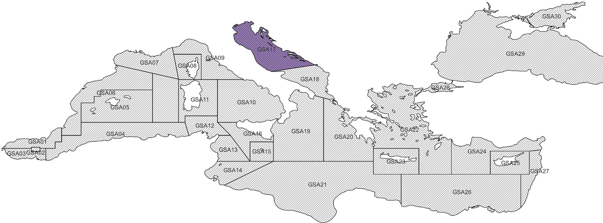
Figure 1 Distribution of Mediterranean geographical subareas (GSAs) of the General Fisheries Commission for the Mediterranean, with the highlight of the GSA-17 addressed by our experiment.

We analysed the 2020 data gaps of four Adriatic commercial stocks targeted by SoleMon: Sepia officinalis, Solea solea, Squilla mantis, and Pecten jacobaeus. To this aim, we introduced a new model to estimate the biomass-index of these stocks in the 2020 missed hauls. Our model combines three sub-models: one sub-model uses a spatial analysis of the surveyed hauls in 2020; a second sub-model processes the historical information on the missed hauls to forecast values in 2020; the third sub-model estimates the environmental suitability of the missed hauls to species persistence. We implemented the three analysis dimensions as different machine learning and statistical models and eventually combined them into one overall model. We trained the sub-models with data up to 2019. Finally, we evaluated model accuracy by forecasting 2019 known data, using data up to 2018 to train the sub-models.

The proposed model is general enough to be re-used for other areas, years, stocks and survey programmes, reconstruct data in time and space, and produce valuable information for stock assessment models.This paper is organised as follows: Section 2 describes our model and sub-models; Section 3 reports our model’s optimal parametrisation and accuracy to predict known 2019 data; Section 4 discusses the results and draws the conclusions.

2 Methods

2.1 Model Overview

This paper proposes a machine learning and statistical modelling solution to reconstruct a biomass density index (biomass over surface, expressed in kg/km²) over a set of survey hauls monitored by SoleMon (Figure 2). We targeted 4 stocks and 10 hauls (over 67) in North-Central Adriatic that were not visited in 2020.

FIGURE 2

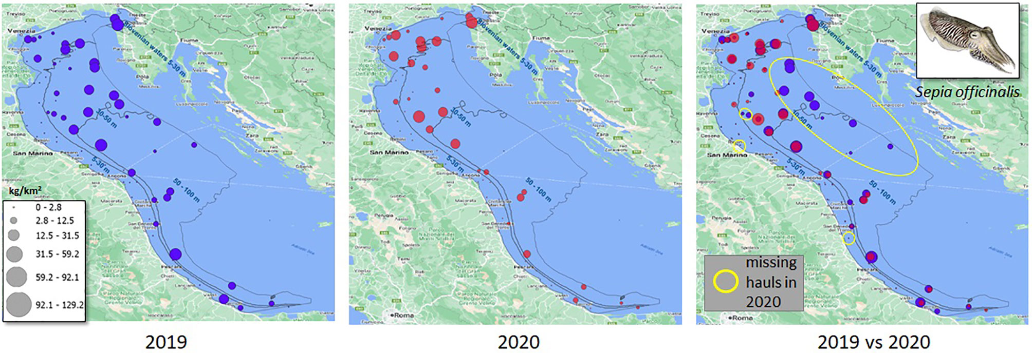
Figure 2 Explanatory example of our model’s scope, i.e., estimating stock biomass-index (Sepia officinalis, in the example) in the hauls missed by the SoleMon programme surveys in 2020. The depth strata used by the total biomass index calculation are also reported.

The premises of our experiment can be summarised as follows:

1. Scientists estimated stock biomass-index for 67 fixed-location hauls between 2006 and 2019. The 2005 survey was structured with another set of hauls and sampling plan, and was thus excluded from the analysis;2. in 2020, biomass-index measurements were missed for 10 hauls; 3. the biomass-indexes of the previous years - with possible sporadic gaps - were available for the unsurveyed haul;4. the survey period was always late fall.

Our goal was to estimate:

1. the biomass-index of each missed haul in 2020 for the 4 selected stock;2. the 2020 total biomass-index for each stock, to be proposed as a fishery-independent tuning index in stock assessment models;3. the contribution of each missed haul to the total biomass-index as an indication of the priority to survey these hauls (haul contribution to total biomass-index);4. the relation between model uncertainty and haul contribution.

We propose a haul biomass-index estimator (HBIE) that combines three components (Figure 3):

FIGURE 3

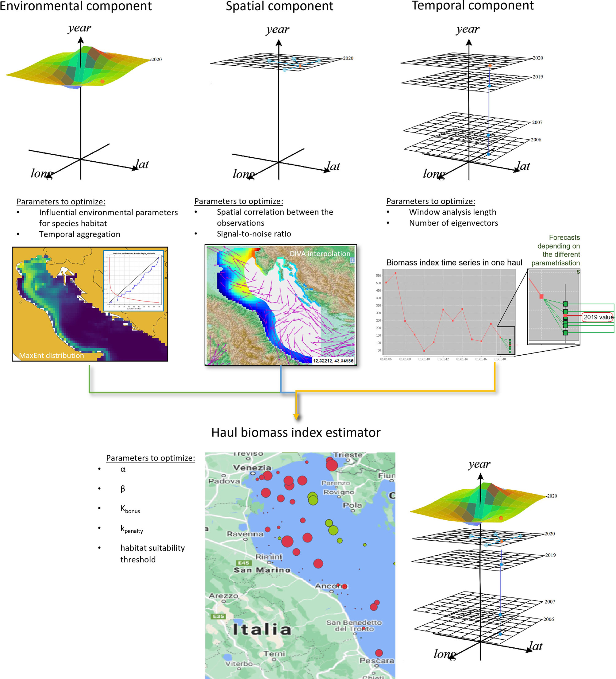
Figure 3 Overview of our overall biomass-index estimation model and its three components, alongside the parameters required by each model.

1. A spatial component that estimates the biomass index of a missed haul given the biomass index of the hauls surveyed in the same year. This model uses oceanographic data to estimate the spatial correlation between the surveyed hauls and the stock biomass index in the missed hauls (Section 2.3);2. A temporal component that forecasts a missed haul’s biomass-index in the analysis year based on the historical biomass-index measurements in that location (Section 2.4). Differently from alternative models, this model can also discover long-term correlations;3. An environmental component that penalises or increments the biomass-index estimates in a missed haul by evaluating if it presents favourable environmental conditions for species presence (Section 2.5). This model represents a novelty in survey data gap filling because it hypothesises that favourable environmental conditions are key factors to compensate for fishing mortality (Froese et al., 2017).

The following sections explain how these components were implemented and combined through machine learning and statistical models and applied to the SoleMon 2020 survey data. Since independent measurements were not available for the missed hauls, model optimisation had to rely on the data at hand. Therefore, we used a precautionary optimisation constraint that assumed that the estimated total biomass-index was not too far from the one measured in the last year (Section 2.7). Abrupt and unpredictable events of stock absence or boost from one year to the next are indeed uncommon, especially in a circumscribed area like the Adriatic (Stergiou and Pollard, 1994; Coro et al.,  2016a).

2.2 Total Biomass-Index Calculation

The total biomass-index produced by the SoleMon surveys is a biomass density index (expressed in kg/km²) based on weighted depth strata, where larger strata have higher weights. It was first introduced by Cochran (1977) and later revised by Souplet (1995). Its calculation was adapted by Grati et al. (2013) to the Adriatic by assigning specific strata weights. This process currently uses three depth strata (at 5-30°m, 30-50°m, and 50-100°m, Figure 2), corresponding to those where the target stocks (mostly flatfishes) are more abundant. Each stratum u is assigned a predefined and fixed weight W (u) proportional to its extension. The input is the set of biomass-indexesb (h, s, y) estimated by a survey campaign for each year y, target stock s, and haul h. The index is the observed biomass (in kg) divided by the haul swept-area (in km²). The total biomass-index tb(s, y) of stock s in year y is calculated by (i) transforming each haul biomass index into a biomass estimate through multiplication with the haul’s swept area, (ii) summing all haul biomass estimates, (iii) dividing the total biomass by the total stratum area (to obtain a stratum biomass-index), and finally (iv) calculating the weighted sum of the stratum biomass-indexes. The following algorithm summarises the process:

Algorithm 1 Total biomass index calculation algorithm for each stock s and year y for each stratum u for each haul h get the swept area a(h,u)calculate the biomass of the haul and stratum: B(h,u,s,y)= b(h,s,y)·a(h,u)calculate the overall stratum biomass across the hauls: $B(u,s,y)={\displaystyle {\sum }_{h}B(h,u,s,y)}$ calculate the overall swept area of the stratum: $A(u)={\displaystyle {\sum }_{h}a(h,u)}$ calculate the biomass-index of the stratum: b(u,s,y)=B(u,s,y)/A(u) calculate total biomass-index as the weighted sum of the strata biomass-indexes: $tb(s,y)={\displaystyle {\sum }_{u}b(u,s,y)·W(u)}$

The main aim of the present experiment was thus to estimate b(h*,s,y) in the hauls ( h*) missed by the SoleMon surveys in 2020, and then calculate tb(s,2020) for 4 target stocks. The time series {tb(s,2006),tb(s,2007),⋯,tb(s,2019),tb(s,2020)} of the 4 stocks was meant to be proposed to the GFCM and STECF working groups as a fishery-independent support to stock assessment models.

2.3 Spatial Component

Our model’s spatial component estimates the stock biomass-index in the hauls missed in a specific survey year (e.g., 2020) given the biomass-index distribution in the surveyed hauls. To this aim, it interpolates the measured biomass-indexes to produce a homogeneous distribution over the area. The model assumes that the measured biomass-indexes are punctual scattered observations of a parameter uniformly defined over the analysed area. It assumes that the spatial correlation between these observations relates to the species’ geographical spread, its ecological region in the water column, and the oceanic currents (Troupin et al., 2010; Watelet et al., 2016). To implement our spatial component, we used the Data-Interpolating Variational Analysis (DIVA) model (Barth et al., 2010). DIVA is typically used to estimate the uniform spatial distribution of a marine parameter from scattered observations, assuming that it is subject to currents and dependent on sea depth (Schaap and Lowry, 2010; Coro et al., 2018a; Coro and Trumpy, 2020). To this aim, DIVA solves the advection equation. As input parameters, it requires a prior estimate of the spatial correlation between the observations and the amount of noise in the data (signal-to-noise ratio) (Troupin et al., 2010; Troupin et al., 2012; Coro et al., 2016b). Internally, the model reconstructs a continuous vector field from the scattered measurements through the Variational Inverse Model (Bennett, 1992). It fits a generic continuous field to the data based on a minimization cost-function (Watelet et al., 2016). The fit algorithm is a finite-element statistical method that uses bathymetry and oceanic-current values in the observation locations as constraints. The fitted field is eventually projected on a regular spatial grid, and a triangular-element mesh is traced over the interpolation area. The characteristic length of the mesh elements is related to the spatial correlation between the input observations.

Our spatial component was a DIVA model, which we trained on the b(h,s,2020) biomass-index available estimates of the SoleMon surveyed hauls in 2020 (57 values). We used the DIVA interpolated values in the 10 missed hauls h* as the biomass-index estimates b(h*,s,2020) of the spatial component. As further input to the DIVA model, we used the 2020 annual water-column averaged oceanic-current components, as NetCDF files, from the Copernicus Global Ocean Physic Analysis (Von Schuckmann et al., 2018). Another input was a bathymetry NetCDF file from the high-resolution GEBCO-2020 dataset (GEBCO, 2020). To speed up processing, we executed the model on the D4Science cloud computing platform (Coro et al., 2015a; Candela et al., 2016; Coro et al., 2017; Assante et al., 2019; Assante et al., 2020) that freely offers the DIVA software for notebook development (Blue Cloud, 2022). The used notebooks and platform are linked in the Supplementary Material.

2.4 Temporal Component

Our temporal component was based on Singular Spectrum Analysis (SSA), a signal processing model to forecast time series values based on long-term sample dependency (Vautard et al., 1992). SSA decomposes the input time series into the sum of simpler time series (hidden components), which represent its hidden structure. It eventually combines these components to reconstruct possible gaps and project the time series in the future. For the present experiment, we used our own open-source JAVA implementation of this algorithm (Coro et al., 2016a), linked in the Supplementary Material.

One SSA main input parameter is the number of samples (M ) of a signal window that contains sufficient information to capture the time series structure. This parameter also represents the maximum temporal dependency between the samples. The algorithm can be summarised as follows (Golyandina and Osipov, 2007; Elsner and Tsonis, 2013):

Algorithm 2 Singular Spectrum Analysis algorithm1. divide the time series X(t) (with t₀≤t≤T) into N sub-segments (chunks) using an M -sample window to cut the signal sequentially;2. build a M×M matrix so that the (i,j) element is the cross-covariance between the i th and j th chunks (lag-covariance matrix);3. extract the lag-covariance matrix eigenvectors {e₁,e₂,…,e_M} and eigenvalues through matrix decomposition;4. project the time series X(t) onto the eigenvectors e_k to estimate its components: $a_k(t)={\displaystyle {\sum }_{j=1}^{M}X(t+j-1)·e_k(j)}$;

5. combine the components {a₁,a₂,…,a_M} to reconstruct the time series (including possible missing samples): $a_k(t)={\displaystyle {\sum }_{j=1}^{M}X(t+j-1)·e_k(j)}$; with N_t being a time-dependent normalization factor;

6. literate the process to forecast additional samples after T.Differently from techniques based on Fourier Analysis, SSA does not use time series frequency information. This feature improves algorithm speed and allows processing also non-stationary time series (Coro et al., 2016a). The estimated eigenvectors represent the time series structure, and each eigenvalue represents the partial variance of the time series in the eigenvector direction. The sum of all eigenvalues is the time series total variance. Reducing the number of eigenvectors for reconstruction and forecast is essential to lowering data noise. The eigenvectors contain essential information about the time series, including noise, but discarding too many of them would generate trivial forecasts. The number of eigenvectors to keep for time series reconstruction and forecast is a crucial parameter to optimize.In our experiment, the optimal SSA parameters for the time series of b(h*,s,t) values (with 2006≤t≤2019) were found for each target stock s and missed haul h* (Section 3.7). The process finally estimated the biomass-index forecasts Xr(t=T+1)= Xr(2020)=b(h*,s,2020). The SSA components {a₁,a₂,…,a_M} were used to fill possible gaps in the time series (which were up to one missing year for each haul) before forecasting data in the future.

2.5 Environmental Component

Our environmental component was based on the Maximum Entropy model (MaxEnt) model, a machine learning-based ecological niche model that estimates species subsistence (i.e., habitat suitability) as a function of environmental parameters (Phillips and Dudík, 2008). MaxEnt can learn from species presence locations only (i.e., without using absence information), which in our case were the hauls surveyed in the analysis year that reported non-zero biomass. We used MaxEnt to simulate the probability that a missed haul fell in suitable habitat for each analysed stock. This probability was used to set a penalty/bonus weight for the biomass estimates produced by the spatial and temporal components (Section 2.6). MaxEnt was trained on expert-identified sea-water parameters potentially correlated (either directly or indirectly) with the analysed stocks (Mancinelli et al., 1998; Zavatarelli et al., 1998; Cibic et al., 2007; Spagnoli et al., 2010; Lotze et al., 2011; Ninˇcevi´c-Gladan et al., 2015), i.e.:

1. average chlorophyll-a in the water column (mg/m³);

2. average mole concentration of dissolved molecular oxygen in the water column (mol/m³);3. average moles of nitrate per unit of mass in the water column (mol/kg);4. average moles of phosphate per unit of mass in the water column (mol/kg);

5. sea-bottom temperature (°C);6. sea-surface temperature (°C);7. average salinity in the water column (PSU);8. bathymetry (m);9. average size of grains in a sediment sample (m).

These data were mainly retrieved from Copernicus (Sauzède et al., 2017; Salon et al., 2019; Clementi et al., 2021; Feudale et al., 2021) to have spatially aligned and verified data. Bathymetry was retrieved from GEBCO-2020 (GEBCO, 2020). Grain size data belonged to CNR historically-collected Adriatic data (Santelli et al., 2017). Data were retrieved for 2019 (for model evaluation) and 2020 (for data gap filling). The spatial resolution was 0.1°, consistent with the average haul swept area. We evaluated different temporal aggregations of the environmental parameters to train MaxEnt: annual (average over the year), seasonal (average per season), trimester (average per trimester), hot-cold months (separate averages for July-September and October-December), and survey period (November-December average). For each species, we also used MaxEnt to select the parameters with the highest correlation with presence and tested them for optimal modelling.MaxEnt is widely used in ecological niche modelling (Raybaud et al., 2015; Capezzuto et al., 2018; Angeletti et al., 2020). It is naturally suited for modelling the distribution of a fixed number of events in a delimited space (such as survey hauls) and is equivalent to a Poisson-regression generalized linear model (Renner and Warton, 2013). In the training phase, MaxEnt estimates a function $\pi \left(\overline{x}\right)$ of environmental parameter vectors $\overline{x}$ constrained to have maxima on species presence locations and minima on simulated absence locations. It is common to consider $\pi \left(\overline{x}\right)$ a proxy of a probability density of species presence (Phillips and Dudík, 2008; Elith et al., 2011; Merow et al., 2013; Coro et al., 2015b, Coro et al., 2018b). Therefore MaxEnt estimates a functional relation between environmental parameters and the species’ presence to generalise the species’ distribution (Pearson, 2007). We trained and tested one MaxEnt model for each target species and every environmental parameter temporal aggregation (Section 2.7).

MaxEnt model inherits the spatial resolution of the environmental parameters (0.1°, in our experiment). The optimization algorithm estimates $\pi \left(\overline{x}\right)$ after maximising the entropy function $H=-\sum ^{\text{}}\pi \left(\overline{x}\right)ln\left(\pi \left(\overline{^x}\right)\right)$ on the training locations (e.g., non-zero biomass surveyed hauls in 2020) with respect to randomly-selected vectors in the study area (background points). During the process, it estimates the coefficients of a linear combination of the environmental parameters that represent the importance of each parameter to predict the species’ distribution (percent contribution). These coefficients can be used to select the parameters carrying the highest quantity of information for the model and re-train/re-test it (Phillips et al., 2017; Coro, 2020a; Coro and Bove, 2022). We used the estimated $\pi \left(\overline{x}\right)$ function to build up a bonus/malus factor for the biomass estimates produced by the other two components (Section 2.6).We used and configured a MaxEnt software implementation (Phillips et al., 2017) (linked in the Supplementary Material) to reduce over-fitting risk by (i) allowing random background point selection (i.e., pseudo-absence location estimation) to possibly include also surveyed hauls with non-zero biomass (Coro et al., 2022a), and (ii) using hinge features to model complex presence-environment relations (Hengl et al., 2009).

2.6 Haul Biomass-Index Estimator

We built the overall haul biomass-index estimator (HBIE) model as an open-source R program (linked in the Supplementary Material) that combined the three components described in the previous sections. Being${\overline{x}}_{h^{*}}$ the set of environmental feature values in missed haul h*, HBIE estimates the biomass-index $b_{HBIE}\left(h^{*},{\overline{x}}_{h^{*}},s,y\right)$ of stock s in year y and haul h* as:

$$\begin{array}{l}{b}_{HBIE}\left(h^{*},{\overline{x}}_{h^{*}},s,y\right)=W\left({\overline{x}}_{h^{*}}\right)·\\ \frac{\alpha ·b_{spatial}\left(h^{*},s,y\right)+\beta ·b_{temporal}\left(h^{*},s,y\right)}{\alpha +\beta }\end{array}$$

where

$$W\left({\overline{x}}_{h^{*}}\right)=\{\begin{array}{l}{k}_{\text{bonus}}if\pi \left({\overline{x}}_{h^{*}}\right)>\text{habitat suitability threshold}\hfill \\ k_{\text{penalty}}\text{\hspace{0.17em}otherwise}\hfill \\ 1\text{\hspace{0.17em}\hspace{0.17em}if environmental information is unavailable}\hfill \end{array}$$

The $W\left({\overline{x}}_{h^{*}}\right)$ term acts as a bonus multiplier if habitat is suitable in h*, and as a penalty factor otherwise. A habitat suitability threshold set on top of the $\pi \left({\overline{x}}_{h^{*}}\right)$ values distinguishes between these two conditions.

In our experiment, we calculated $b_{HBIE}\left(h^{*},{\overline{x}}_{h^{*}},s,2020\right)$ for the 4 selected SoleMon stocks in the 10 hauls missed in 2020, but the HBIE model could be applied beyond the SoleMon data. Generally, it is applicable to stocks and survey data with temporal, spatial, and environmental information associated. It would work even if either the spatial or the temporal components were missing. Additionally, if environmental data were missing, the corresponding component factor would be 1.HBIE introduces new parameters to be estimated in the optimization phase (Section 2.7), i.e., α; β ; k_bonus; k_penalty, and the habitat suitability threshold.

2.7 Model Optimization and Evaluation

2.7.1 Optimisation

The complete list of parameters to optimise is reported in Table 1. Of course, the optimal parametrisation depends on the stock. We translated the precautionary modelling assumption explained in Section 2.1 into the assumption that the optimal model was the one producing the minimum total biomass-index difference with respect to the last year. Therefore, in our case the optimised parameters were those that ended in the minimum total biomass-index difference between 2019 and 2020.

TABLE 1

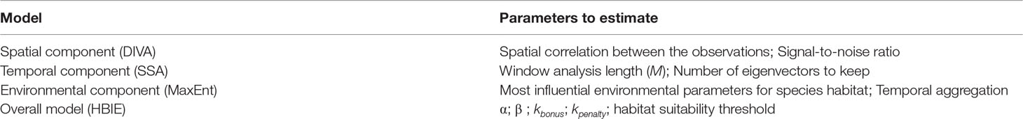
Table 1 Complete set of parameters used by our models and optimised in the training phase.

To select the optimal DIVA parametrisation, we fit DIVA to the biomass-indexes of the 57 surveyed hauls of 2020 by testing several combinations of spatial correlation and signal-to-noise values. We searched for the parameters that minimised the difference between the total biomass-index in 2020 and 2019 after the DIVA estimations. DIVA embeds the DIVAfit tool, a statistical tool that produces an initial estimate of the parameters. This tool estimates spatial correlation after fitting the target vector field to the data, under spatial homogeneity hypothesis. It also estimates signal-to-noise ratio based on the anomaly range of this fit (Troupin et al., 2010). Based on the DIVAfit indications on our data, we tested spatial correlations between 0.5° and 2° (by 0.5°steps) and signal-to-noise ratios between 0.1 and 10 (by 0.2° steps).

We trained SSA for each of the 10 missed hauls separately to select the optimal temporal component parametrisation. We used historical biomass-index data from 2006 to 2019 (i.e., 14 values) to forecast the 2020 haul biomass-index. We selected the individual-haul parameters minimising the total biomass-index difference between 2020 and 2019. The optimal temporal correlation and number of eigenvectors depended on the haul and the stock. Thus, we optimised 4 stocks×10 hauls=40 SSA models. For each model, we tested all analysis window lengths between 2 (short-term dependency) and the maximum length of the time series (long-term dependency). We also iteratively incremented and tested the number of eigenvectors to keep for the forecast (Ding et al., 2008).

To select the optimal environmental component parametrisation, we used the non-zero biomass hauls in 2020 as observation locations and tested different environmental parameter sets and temporal aggregations. We tested annual, seasonal, trimester, hot-cold months, and survey period aggregations of the 9 parameters listed in Section 2.4. The non-zero biomass locations used as observation records were 31 for S. officinalis, 51 for S. solea, 51 for S. mantis, and 11 for P. jacobaeus. MaxEnt was configured to generate a maximum of 1000 background points as pseudo-absence locations and conduct 500 training iterations. Following the indications to reduce over-fitting risk reported in Section 2.5, pseudo-absence locations were randomly taken with the possible inclusion of the surveyed hauls, and hinge feature usage was enabled. The projection area was made up of ~ 2900 locations. In the selection process, we first identified the optimal temporal aggregation by tracing the Receiver Operating Characteristic (ROC) curve. This curve allowed us to conduct a sensitivity analysis by calculating true-positive and false-positive rates using various decision thresholds on the model output. The ROC curve integral is the Area Under the Curve (AUC) and was used as a model-selection criterion (Coro et al., 2015b; Coro et al., 2018b). The higher the AUC, the better the model because a high AUC indicates that the model simulates a probability distribution with significantly higher values on species-presence locations than on random locations. To further test the parameter set, we compared the model using all variables against one using the features carrying 95% of the total percent contribution (Coro et al., 2015b). Eventually, we selected the model with the highest AUC. The habitat suitability threshold used by the HBIE model was the number that resulted in an omission rate (percentage of false absences over estimated absences) below 1% (Coro and Trumpy, 2020; Coro, 2020a; Coro and Bove, 2022).

After optimising the individual components, we optimised the HBIE model by testing all parameter combinations within the following prior ranges: [0.1;2] (by 0.1 steps) for α and β; [0;2] (by 0.1 steps) for kbonus and kpenalty. Eventually, we selected the set resulting in the minimum total biomass-index difference between 2020 and 2019.

2.7.2 Evaluation

In order to evaluate the HBIE model, we used 2019 as the analysis year and hypothesised that the missed hauls were the same 10 hauls missed in 2020. We used the time series of 2006-2018 data of these hauls (i.e., 13 values for each haul) to train the temporal component and forecast the 2019 values. We used 57 biomass-index values in 2019 (i.e., those from the same surveyed hauls of 2020) to train the spatial component and project its estimates in the missed hauls. The same 57 locations were used as observation records (when biomass-index was non-zero) to train the environmental component with the 9 selected environmental parameters and, iteratively, on 5 temporal aggregations (from annual to November-December period). We used 2019 values for all environmental and oceanic parameters involved. Non-zero biomass observation records were 32 for S. officinalis, 52 for S. solea, 32 for S. mantis, and 17 for P. jacobaeus. MaxEnt was configured to generate a maximum of 1000 background points as pseudo-absence locations and 500 training iterations.

We used the measured 2019 biomass-indexes in the missed hauls to calculate model accuracy, i.e., the percentage of correctly predicted indexes within statistical confidence limits. We also estimated the correct prediction of the 2019 total biomass-index.

As a baseline comparison index, we adopted an equiproportional index that assumed, for each missed haul, that the average ratio between the total biomass-index of the surveyed hauls and the missed hauls’ index remained constant over the years. Therefore, after calculating the average ratio for each unsurveyed haul, this index easily allowed estimating the unsurveyed hauls’ values. The equiproportional index calculation algorithm is summarised as follows:

Algorithm 3 Equiproportional index calculation algorithmfor each missed haulfor each year before the analysis yearestimate the ratio between the total biomass-index in the surveyed hauls and the biomass-index in the missed haulaverage the ratios over the yearsuse the ratio to estimate the biomass-index in the missed haul, in the analysis year, given the total biomass-index of the surveyed haulsestimate the total biomass-index using the surveyed values and the estimates for the missed hauls

We also analysed the relation between our HBIE model uncertainty and the hauls’ contributions to the total biomass-index. Haul contribution was estimated as the average relative variation of the total biomass-index over the years when the haul (and its associated strata) was removed from the calculation. Evaluating the relation between haul contribution and HBIE model precision shed light on accuracy calculation reliability and stock biomass distribution homogeneity. It is worth noting that HBIE uncertainty comes from the DIVA model after propagating the confidence limits into the HBIE formula. In fact, the canonical SSA algorithm does not produce statistical uncertainty for its estimates (Allen and Smith, 1997) and MaxEnt was used as a thresholded factor.

3 Results

3.1 Optimal Parameters

The optimal model parameters for the 2020 SoleMon data are reported in Table 2. The DIVA spatial correlation reflects the average spatial geographical distance from an abundant location to the other, with less mobile species (e.g., P. jacobaeus) having lower spatial correlation values. The signal-to-noise ratio was averagely low for all species, but was sensibly higher for S. solea. The average SSA temporal dependencies indicate that long-term dependency modelling (from 7 to 9 years) was necessary for good forecasts. MaxEnt gave optimal results when all parameters were used because they all brought essential information to properly model species presence. The optimal temporal aggregation was hot and cold months (i.e., separate averages over July-September and October-December). Cold months indeed included the environmental conditions of the survey period, and hot months included summer conditions that might have influenced species distribution in winter (Henderson et al., 2017). The MaxEnt habitat suitability threshold depended on the species. Interestingly, these values almost corresponded to the lower confidence limit of a log-normal distribution traced over all MaxEnt values on low-biomass locations. In this case, low-biomass locations were those with a biomass-index falling at the lower log-normal tail of the overall biomass-index distribution.

TABLE 2

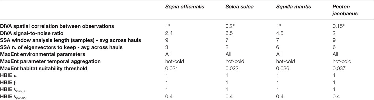
Table 2 Optimal model parameters estimated for the analysed stocks based on the SoleMon data.

The HBIE optimal parameter values indicate that no component outperformed the other. Therefore the weighted average in the HBIE formula was a standard average. This condition was likely related to the specific SoleMon data, with few temporal gaps and a peculiarly invariant haul distribution over the years. We anticipate that conditions such as worse temporal sampling, less homogeneous spatial sampling, and under-representative data would result in different component weights. The environmental suitability bonus was 1 for all species, which indicates that the models directly reported the average biomass-index estimate for suitable habitat locations in the analysis year. Instead, all models applied a 0.4 penalty (i.e., a 60% reduction) on unsuitable habitat locations. Therefore, the environmental component only intervened in unsuitable habitat hauls to soften the biomass-index estimate.

Two examples on S. officinalis missed hauls show the difference between the HBIE model and its components (Figure 4). The first example reports a haul’s historical biomass-index with tri-annual periodicity between 2011 and 2017. The equiproportional index coarsely identified a decreasing trend in the last years and thus estimated a slightly lower value for 2020 (32.9 kg/km²) than the 2019 value (33.48 kg/km²). Our spatial component also estimated a slightly lower value for 2020 (32.62 kg/km²) than the 2019 value. The temporal component better captured the decreasing trend in 2020 and reported a 23% lower value (25.11 kg/km²) than the other indexes. The environmental component classified the habitat as unsuitable for the species in the haul in 2020, and thus further decreased the estimated biomass-index to 11.55 kg/km². This penalty resulted in better capturing the low biomass that experts expected in the haul due to a delayed species absence periodicity and unsuitable habitat. It is worth noting that habitat was instead suitable in 2019, with a relatively high biomass-index (33.48 kg/km²), and all HBIE components achieved a good prediction of this value (between 33.11 and 36.2 kg/km²). Instead, the equipropotional index overestimated the 2019 value as 44.9 kg/km².The second example shows a particular non-periodical biomass-index time series associated with a missed haul. The equiproportional index estimate for 2020 (24.7 kg/km²) was higher than the 2019 value (16.13 kg/km²) because it captured an averagely increasing trend since 2012. The spatial model reported a similar estimate for the same year (24.95 kg/km²). Instead, the unpredictability of the time series of the last years made the temporal component estimate complete stock absence in the haul for 2020. Since habitat was estimated as suitable in the haul area in 2020, HBIE directly returned half of the spatial model estimate as the final result without further penalties (12.47 kg/km²). This estimate compensated for the potential bias of the temporal component. It is worth noting that this value is consistent with the time series values because it is close to the last 10-year average (14.3 kg/km²), if the 2018 value (55.63 kg/km²) were considered an anomaly. The evaluation of the 2019 value prediction shows that all HBIE components returned very close values (from 15.8 to 16.04 kg/km²) to the real value (16.13 kg/km²), whereas the equiproportional index sensibly overestimated it (34.34 kg/km²). The temporal component prediction was particularly close to the real value, which demonstrates the SSA effectiveness with non-stationary time series, but - considering the 2020 estimate - also its sensitivity on the number of samples and abrupt variations. All the time series comparisons for the missed hauls are reported in the Supplementary Material.

FIGURE 4

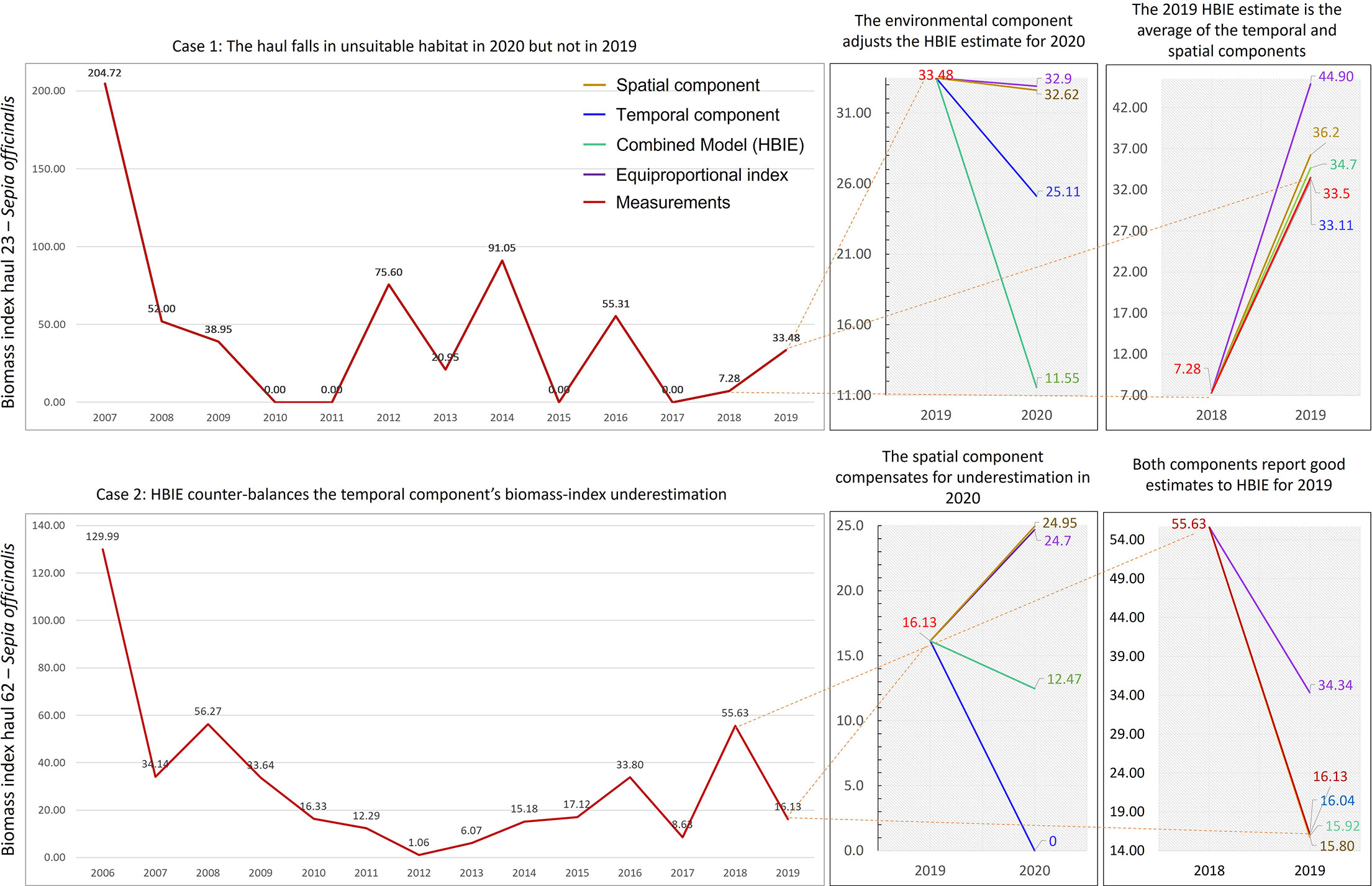
Figure 4 Two cases demonstrating substantial differences between the biomass-index estimates of our combined model (HBIE) and its temporal and spatial components with respect to a baseline estimate (equiproportional index). The two cases show a quasi-periodic and a non-periodical time series, respectively. The rightmost charts report forecasts of 2019 values and comparison with known data. The middle charts report forecasts of 2020 values. The dashed lines highlight the correspondence between the measurements (real data) and the same points in the forecast charts. The colours of the numbers and lines in the forecast charts correspond to the legend indications.

3.2 Performance

We trained a model using 2019 data, while excluding the same hauls missing in 2020. We used the 2006-2018 data for time series analyses and took 2018 data as a reference for model training. Since temporal and spatial sampling data were constant in the surveyed area over the years, the estimated optimal HBIE parametrisation - apart from the habitat suitability thresholds - was equal to the one for 2020 data (Table 2). The MaxEnt environmental parameters were all confirmed to carry important information for optimal modelling. The hot-cold-months aggregation was confirmed to be optimal, and thus was not specific to the 2020 data. The average SSA and the DIVA parameters were not sensibly different from the 2020 model’s ones, thus they only depended on the spatiotemporal structure of the data.

Average accuracy on haul-biomass recognition ranged from 80% to 100% (Table 3), which was higher than the 30%-80% range of the equiproportional index. The lowest accuracy was obtained for S. mantis, and was probably due to the very low biomass in the missed hauls, going down to complete absence in some cases. The total biomass-index fell within the confidence ranges for all stocks, whereas the equiproportional index correctly estimated the total biomass-index of P. jacobaeus only. The comparison table also reports the estimated 2020 total biomass-indexes, which are meant to feed RFMOs’ stock assessment models (Froese et al., 2020).The overall biomass-index distributions are displayed in Figure 5.

TABLE 3

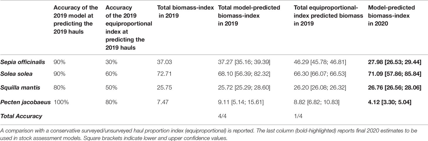
Table 3 Performance of our model with respect to measured 2019 biomass-indexes across the four analysed stocks.

FIGURE 5

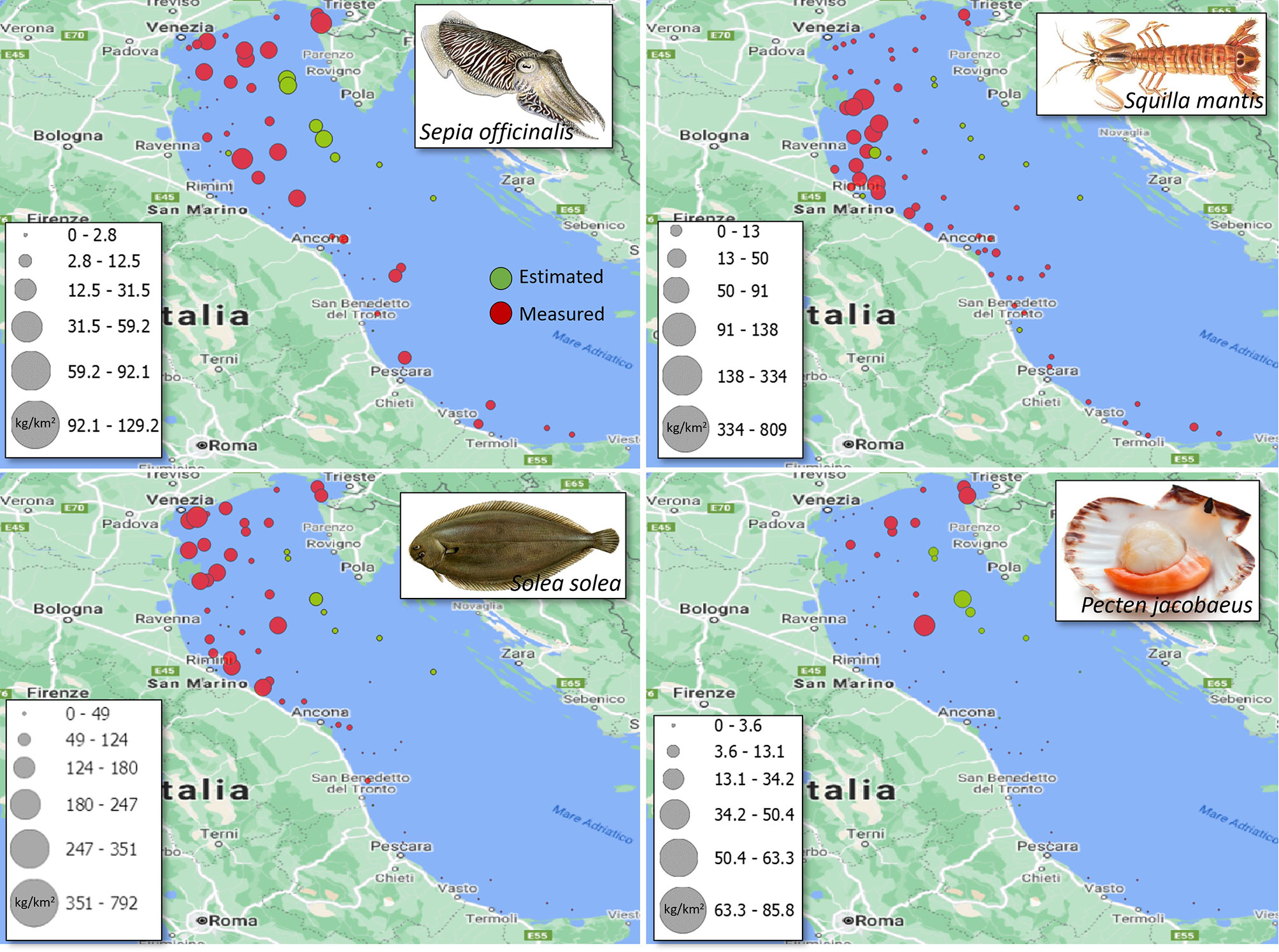
Figure 5 Distribution of measured (red) and estimated (green) SoleMon biomass-indexes per haul for 2020.

3.3 Model Uncertainty and Haul Contribution to Total Biomass-Index

Highly contributing hauls to the total biomass-index were present throughout the entire area (Figure 6). However, no stock presented an isotropic and homogeneous distribution of highly contributing hauls. One small homogeneous area of lowly contributing hauls can only be observed for S. mantis in the deep area halfway between the Italian and Croatian coasts.

FIGURE 6

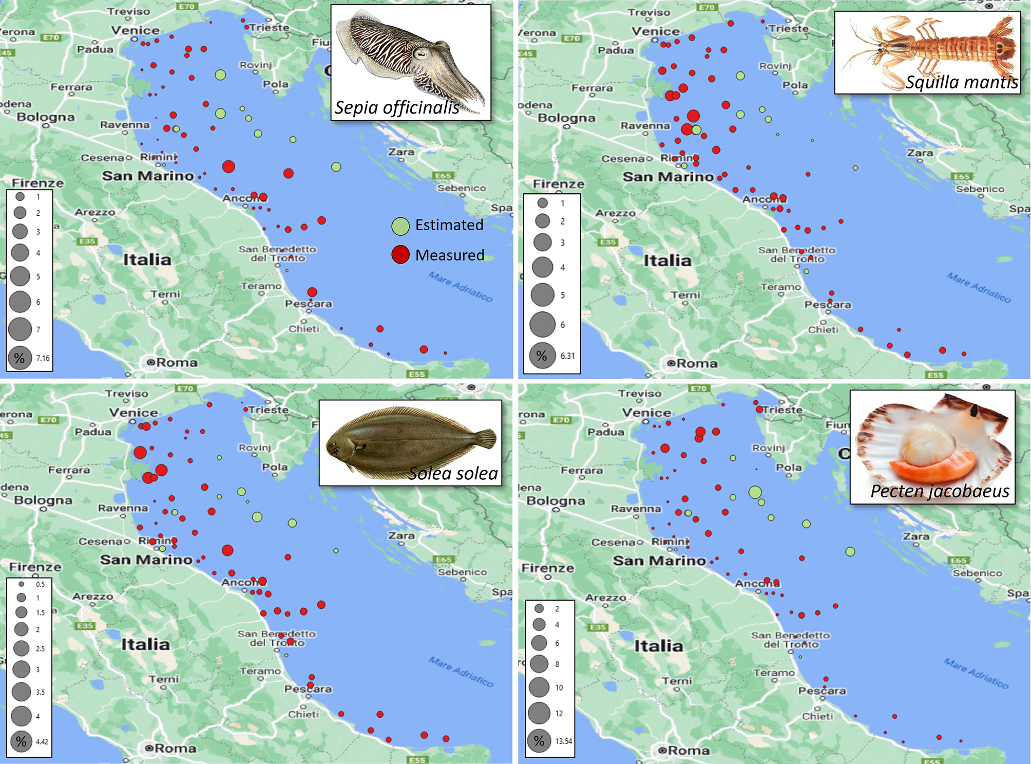
Figure 6 Percent average contributions, over the survey years, of the SoleMon hauls to the total biomass-index. Colours highlight the 2020 measured (red) and estimated hauls (green).

It is worth noting that the unsurveyed 2020 hauls were not randomly distributed, but mostly concentrated off the Croatian coasts with generally high contributions to the total biomass index. Therefore, it was crucial to estimate these values correctly because they sensibly influenced the total biomass-index estimates.

Due to inhomogeneous distribution, low-contribution locations could reside very close to high-contribution locations because low-biomass hauls could surround large-biomass hauls. Therefore, high-contribution hauls were peaks of the contribution distribution close to minima. This scenario increased the estimation uncertainty on high-contribution hauls. This observation is confirmed by a direct linear relation between the 2020 HBIE model uncertainty and the haul contribution to the total biomass-index (Figure 7). The correlation strengths range between moderate (0.36 for S. solea, 0.44 for P. jacobaeus, and 0.46 for S. officinalis) and high (0.95 for S. mantis). The higher the contribution, the higher the uncertainty. Understanding this relationship is important when re-using our model for other stocks and areas. Generally, this relation complies with the expected properties of a biomass estimation model. It is reasonable that such a model predicts missing data with higher precision over a small area with homogeneous biomass, and with lower precision over a wide area with jeopardised large-biomass distribution.

FIGURE 7

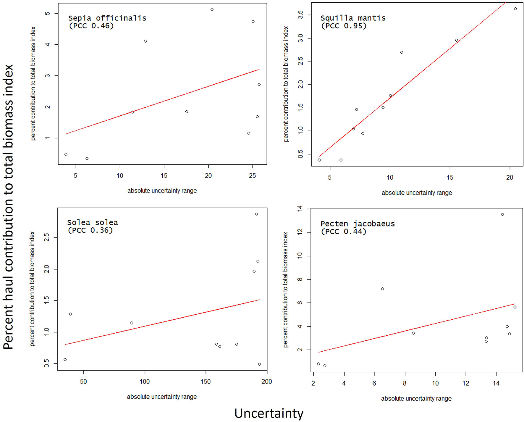
Figure 7 Linear fit between the HBIE 2020 model uncertainty and the percent haul contribution to the total biomass, with the indication of the Pearson Correlation Coefficient (PCC).

4 Discussion and Conclusions

We have presented a model to estimate stock biomass density in occasionally unsurveyed areas, with an application to the 2020 SoleMon survey data in North-Central Adriatic Sea. The model combines three complementary components: spatial, temporal, and environmental. When applied to the 2019 SoleMon data, our model was able to estimate the total biomass-index of all analysed stocks correctly. The accuracy over individual haul biomass-index estimation was also high (80-100%). We observed that model uncertainty was higher for larger biomass-index hauls, probably because of the jeopardised biomass distribution of the analysed stocks. Moreover, the model achieved a higher estimation accuracy than an alternative, widely used index that assumed the conservation of average surveyed/unsurveyed biomass proportion over time. The advantage of this alternative index is its fast implementation, but our results showed that it is more suited for coarse approximations. Our model implementation is fully based on open-source software, and every sub-model is available either as desktop software or notebook (Supplementary Material). After data preparation, running the sub-models for one species on a modern desktop PC or laptop - e.g., endowed with an Intel i9 CPU with 8 GB of Random Access Memory - requires about 1 hour. Moreover, all sub-models can be used through free-to-use Web interfaces based on cloud computing systems that simplify model configuration and speed up data processing. One limitation of our current implementation is that the three sub-models are not integrated into an all-in-one offline process because DIVA is currently released as a notebook that can be hardly transformed into an automatic process. Our next-future plan is to transform DIVA into a Web service to facilitate its automatic integration with the other sub-models, which will require preparing specific cloud services and infrastructures (Assante et al., 2020).

One similarity between our model and VAST is that they both include spatial and temporal models, although they are modelled and combined differently. VAST uses two functions to estimate stock biomass density in the unsurveyed hauls for a specific survey year: one is the probability p(s_i,t_j) of encountering the species in unsurveyed haul s_i in year t_j, and the other is the expected catch rate r(s_i,t_j). The expected stock biomass density d(s_i,t_j) in s_i is calculated as the product of these two terms, i.e., d(s_i,t_j)=p(s_i,t_j)·r(s_i,t_j). VAST models p(s_i,t_j) as a logit distribution approximated by a linear combination of unknown random variables defined on s_i and t_j. Moreover, it models r(s_i,t_j) as the mean of a log-normal distribution approximated by another linear combination of random variables. The probability ( p) of encountering the species in the unsurveyed hauls in the analysis year coarsely corresponds to our environmental and spatial components, although VAST does not explicitly use environmental variables. The VAST catch rate term ( r) is a time-dependent model that, differently from our temporal component, does not estimate a biomass index directly. Moreover, being d the product of the two r and p terms, the two models should be very accurate because multiplication is highly sensitive to individual function biases. Conversely, in our model, one of the biomass-index estimators could even be missing. Finally, VAST finds the optimal distributions using the Akaike Information Criterion as a model quality measurement, which introduces the potential bias to always select models with a higher number of parameters among equal-likelihood models (Guthery et al., 2005; Arnold, 2010; Coro et al., 2022a). Conversely, our model trains the components independently of each other using the last known biomass index as a reference. Moreover, each component models a more complex function than a linear combination of random variables.Our model shares characteristics with general spatiotemporal data gap filling models for remote sensing imagery reconstruction, which separately fill spatial and temporal gaps and eventually combine the estimates (Weiss et al., 2014; Metz et al., 2017; Yan and Roy, 2018). With respect to these models, our model uses an ocean-specific kriging model for spatial modelling. Moreover, it uses a general signal processing technique for temporal modelling that is more complex than the pixel-wise temporal smoothing functions used by most alternative models. One interesting comparison is with deep-learning-based models that directly simulate a space-time data reconstruction function and can reach very high performance in specific contexts (Belda et al., 2020; Varshney et al., 2021; Goodman, 2021). Differently from our model, deep-learning models can difficultly be re-implemented and adapted to new contexts - that usually require new model topologies and specific large training sets - and optimisation is very time-consuming. Moreover, performance and bias interpretability are easier for our type of model components than for deep learning models (Chakraborty et al., 2017; Zhang and Zhu, 2018).We conjecture that our model is general enough to be applied also to other fishery trawl survey data. However, we acknowledge that the performance on SoleMon data were facilitated by favourable conditions such as a low inter-annual spatio-temporal variability of the haul distribution. Unfortunately, such conditions are uncommon and unlikely in more extended and multi-country survey programmes. For example, the Mediterranean MEDITS programme (Spedicato et al., 2019) is a 30-year data collection action that has been subject to changes due to revisions, optimisation, and re-planning. These changes corresponded to data gaps and inhomogeneity in time and space. Our model can manage this scenario by giving the highest weight to the component using the most informative data. Generally, in our future applications we will test our model on survey data that include issues such as (i) haul distribution change across the years, (ii) survey season change, and (iii) haul historical data containing several gaps. A potential limitation of our model when applied to other trawl surveys is that it cannot predict stock abundance directly, which will require integrating more data with the model.

We believe that our model can improve the quality of the information used by the GFCM, STECF, and MSFD, and improve stock status evaluation. Indeed, the biomass indexes reported in Table 3 have already been proposed and used for the 2022 GFCM stock assessments, after experts’ consistency evaluation of the model (Scientific Advisory Committee on Fisheries, 2022).

4.1 Model Applications

The major applications of our model can be summarised as follow:

Data enhancement: The estimated biomass indexes can independently enrich the data coming from fishery survey, especially when major issues prevented complete monitoring. They also help monitor the correlation between biomass distribution and environmental conditions;

Re-application to other scientific survey data: other scientific survey programmes can reuse our models to reconstruct biomass-indexes and compare the results to their current estimates;

Haul contribution analysis: In critically limiting survey conditions, surveys could be prioritised to visit the hauls with the highest contribution to the total biomass-index calculation;

Supporting stock assessment and harvest control rules: Stock status assessment is the basis for setting management rules, i.e., the amount of days fishing vessels can spend at sea and the harvest control rules that limit the catches. Indexes of relative abundance – such as the survey biomass index - are primary input data for stock assessment (Maunder and Punt, 2004). Using robust model-based input data is encouraged when raw observations are not sufficiently reliable (Thorson and Haltuch, 2019). Having access to complete time series with spatial gaps reliably filled would help experts parametrise stock assessment models and increase result reliability and precision;

Understanding the interplay between environmental change and fisheries: Environmental change may affect stock distribution and productivity (Free et al., 2019). The stock-specific intrinsic rate of increase and carrying capacity depend on the interaction between the species and the environment where it lives (Froese et al., 2017). Understanding the interplay between environmental conditions and stock dynamics is crucial for integrated environmental assessment and ecosystem approaches to fishery management (Antunes and Santos, 1999; Rosenberg et al., 2000; Karp et al., 2019; Marshall et al., 2019; Coro et al., 2021). Our model can contribute to this context because it can model species’ habitat suitability change over the years and attach this information to the survey data.

Data Availability Statement

All datasets and software presented in this study can be found in a GitHub free access online repository, which corresponds to the Supplementary Material of the manuscript: https://github.com/cybprojects65/SoleMonGeospatialModelling.

Author Contributions

GC conceived, designed and implemented the model, and conducted the experiments; PB contributed to model design and conducted the experiments; EA and FM provided and prepared biomass and environmental data, and contributed to modelling context definition, environmental parameter selection and result interpretation; MS provided data on Squilla mantis; GS supervised and organised the SoleMon survey campaigns, validated the data and provided information about the surveys. All authors contributed to paper writing and revision.

Funding

This work has been funded by the EcoScope European project within the H2020-EU.3.2.-SOCIETAL CHALLENGES programme, with Grant Agreement ID 101000302. EA, FM, and MS worked in the research leading to these results while enrolled in the Ph.D. Program “Innovative Technologies and Sustainable Use of Mediterranean Sea Fishery and Biological Resources – FishMed”.

Conflict of Interest

The authors declare that the research was conducted in the absence of any commercial or financial relationships that could be construed as a potential conflict of interest.

Publisher’s Note

All claims expressed in this article are solely those of the authors and do not necessarily represent those of their affiliated organizations, or those of the publisher, the editors and the reviewers. Any product that may be evaluated in this article, or claim that may be made by its manufacturer, is not guaranteed or endorsed by the publisher.

References

Aeberhard W. H., Mills Flemming J., Nielsen A. (2018). Review of State-Space Models for Fisheries Science. Annu. Rev. Stat Its Appl. 5, 215–235. doi: 10.1146/annurev-statistics-031017-100427

CrossRef Full Text | Google Scholar

Allen M. R., Smith L. A. (1997). Optimal Filtering in Singular Spectrum Analysis. Phys. Lett. A 234, 419–428. doi: 10.1016/S0375-9601(97)00559-8

CrossRef Full Text | Google Scholar

Angeletti L., Prampolini M., Foglini F., Grande V., Taviani M. (2020). “Cold-Water Coral Habitat in the Bari Canyon System, Southern Adriatic Sea (Mediterranean Sea),” in Seafloor Geomorphology as Benthic Habitat (Amsterdam, The Netherlands: Elsevier ), 811–824. doi:

Google Scholar

Antunes P., Santos R. (1999). Integrated Environmental Management of the Oceans. Ecol. Economics 31, 215–226. doi: 10.1016/S0921-8009(99)00080-4

CrossRef Full Text | Google Scholar

Arnold T. W. (2010). Uninformative Parameters and Model Selection Using Akaike’s Information Criterion. J. Wildlife Manage. 74, 1175–1178. doi: 10.1111/j.1937-2817.2010.tb01236.x

CrossRef Full Text | Google Scholar

Assante M., Candela L., Castelli D., Cirillo R., Coro G., Dell’Amico A., et al. (2020). Virtual Research Environments Co-Creation: The D4science Experience. Concurrency Computation: Pract. Exp., 35: e6925. doi: 10.1002/cpe.6925

Google Scholar

Assante M., Candela L., Castelli D., Cirillo R., Coro G., Frosini L., et al. (2019). Enacting Open Science by D4science. Future Generation Comput. Syst. 101, 555–563. doi: 10.1016/j.future.2019.05.063

CrossRef Full Text | Google Scholar

Barth A., Alvera-Azcárate A., Troupin C., Ouberdous M., Beckers J.-M. (2010). A Web Interface for Griding Arbitrarily Distributed in Situ Data Based on Data-Interpolating Variational Analysis (Diva). Ad. Geo.28, 29-37 doi: 10.5194/adgeo-28-29-2010

CrossRef Full Text | Google Scholar

Belda S., Pipia L., Morcillo-Pallarés P., Rivera-Caicedo J. P., Amin E., De Grave C., et al. (2020). DATimeS: A Machine Learning Time Series GUI Toolbox for Gap-Filling and Vegetation Phenology Trends Detection. Environ. Model. Software 127, 104666. doi: 10.1016/j.envsoft.2020.104666

CrossRef Full Text | Google Scholar

Bennett A. F. (1992). Inverse Methods in Physical Oceanography ( Cambridge University Press).

Google Scholar

Bergenius M., Eigaard O. R., Orio A., Søvik G., Ulmestrand M. (2021). Joint NAFO/ICES Pandalus Assessment Working Group (NIPAG) Report. Tech. rep., International Council for the Exploration of the Sea (ICES).

Google Scholar

Blue Cloud (2022). The Blue Cloud Lab D4Science Virtual Research Environment.

Google Scholar

Breivik O. N., Aanes F., Søvik G., Aglen A., Mehl S., Johnsen E. (2021). Predicting Abundance Indices in Areas Without Coverage With a Latent Spatio-Temporal Gaussian Model. ICES J. Mar. Sci. 78, 2031–2042. doi: 10.1093/icesjms/fsab073

CrossRef Full Text | Google Scholar

Candela L., Castelli D., Coro G., Pagano P., Sinibaldi F. (2016). Species Distribution Modeling in the Cloud. Concurrency Comput. Pract. Exp. 28, 1056–1079. doi: 10.1002/cpe.3030

Google Scholar

Capezzuto F., Sion L., Ancona F., Carlucci R., Carluccio A., Cornacchia L., et al. (2018). Cold-Water Coral Habitats and Canyons as Essential Fish Habitats in the Southern Adriatic and Northern Ionian Sea (Central Mediterranean). Ecol. Questions 29, 9–23. doi: 10.12775/EQ.2018.019

CrossRef Full Text | Google Scholar

Chakraborty S., Tomsett R., Raghavendra R., Harborne D., Alzantot M., Cerutti F., et al. (2017). “Interpretability of Deep Learning Models: A Survey of Results,” in 2017 IEEE Smartworld, Ubiquitous Intelligence & Computing, Advanced & Trusted Computed, Scalable Computing & Communications, Cloud & Big Data Computing, Internet of People and Smart City Innovation (Smartworld/SCALCOM/UIC/ATC/CBDcom/IOP/SCI) ( IEEE), 1–6.

Google Scholar

Cibic T., Blasutto O., Falconi C., Umani S. F. (2007). Microphytobenthic Biomass, Species Composition and Nutrient Availability in Sublittoral Sediments of the Gulf of Trieste (Northern Adriatic Sea). Estuarine Coast. Shelf Sci. 75, 50–62. doi: 10.1016/j.ecss.2007.01.020

CrossRef Full Text | Google Scholar

Clementi E., Aydogdu A., Goglio A., Pistoia J., Escudier R., Drudi M., et al. (2021). Mediterranean Sea Physical Analysis and Forecast (Cmems Med-Currents, Eas6 System) (Version 1) ( Copernicus Monitoring Environment Marine Service (Brussels, Belgium: CMEMS). doi: 10.25423/CMCC/MEDSEA

CrossRef Full Text | Google Scholar

Cochran W. G. (1977). Sampling Techniques (New York: Wiley).

Google Scholar

Colloca F., Garofalo G., Bitetto I., Facchini M. T., Grati F., Martiradonna A., et al. (2015). The Seascape of Demersal Fish Nursery Areas in the North Mediterranean Sea, a First Step Towards the Implementation of Spatial Planning for Trawl Fisheries. PLos One 10, e0119590. doi: 10.1371/journal.pone.0119590

PubMed Abstract | CrossRef Full Text | Google Scholar

Coro G. (2013). A Lightweight Guide on Gibbs Sampling and JAGS. Tech. rep. Istituto di Scienza e Tecnologie dell’Informazione A. Faedo - CNR. 1–16

Google Scholar

Coro G. (2020a). A Global-Scale Ecological Niche Model to Predict Sars-Cov-2 Coronavirus Infection Rate. Ecol. Model. 69:431, 109187. doi: 10.1016/j.ecolmodel.2020.109187

CrossRef Full Text | Google Scholar

Coro G. (2020b). Open Science and Artificial Intelligence Supporting Blue Growth. Environ. Eng. Manage. J. (EEMJ) 19, 1719-1729. doi: 10.30638/eemj.2020.162

CrossRef Full Text | Google Scholar

Coro G., Bove P. (2022). A High-Resolution Global-Scale Model for Covid-19 Infection Rate. ACM Transactions on Spatial Algorithms and Systems (TSAS)8, 1–24. doi: 10.1145/3494531

CrossRef Full Text | Google Scholar

Coro G., Bove P., Ellenbroek A. (2022a). Habitat Distribution Change of Commercial Species in the Adriatic Sea During the Covid-19 Pandemic. Ecol. Inf., 101675. doi: 10.1016/j.ecoinf.2022.101675

CrossRef Full Text | Google Scholar

Coro G., Candela L., Pagano P., Italiano A., Liccardo L. (2015a). Parallelizing the Execution of Native Data Mining Algorithms for Computational Biology. Concurrency Computation: Pract. Exp. 27, 4630–4644. doi: 10.1002/cpe.3435

CrossRef Full Text | Google Scholar

Coro G., Ellenbroek A., Pagano P. (2021). An Open Science Approach to Infer Fishing Activity Pressure on Stocks and Biodiversity From Vessel Tracking Data. Ecol. Inf. 64, 101384. doi: 10.1016/j.ecoinf.2021.101384

CrossRef Full Text | Google Scholar

Coro G., Large S., Magliozzi C., Pagano P. (2016a). Analysing and Forecasting Fisheries Time Series: Purse Seine in Indian Ocean as a Case Study. ICES J. Mar. Sci. 73, 2552–2571. doi: 10.1093/icesjms/fsw131

CrossRef Full Text | Google Scholar

Coro G., Magliozzi C., Ellenbroek A., Pagano P. (2015b). Improving Data Quality to Build a Robust Distribution Model for Architeuthis Dux. Ecol. Model. 305, 29–39. doi: 10.1016/j.ecolmodel.2015.03.011

CrossRef Full Text | Google Scholar

Coro G., Pagano P., Ellenbroek A. (2018a). Detecting Patterns of Climate Change in Long-Term Forecasts of Marine Environmental Parameters. Int. J. Digital Earth, 13: 1–19. doi: 10.1080/17538947.2018.1543365

CrossRef Full Text | Google Scholar

Coro G., Pagano P., Napolitano U. (2016b). Bridging Environmental Data Providers and Seadatanet Diva Service Within a Collaborative and Distributed E-Infrastructure. Bollettino di Geofisica Teorica ed Applicata, 57: 23–25.

Google Scholar

Coro G., Panichi G., Scarponi P., Pagano P. (2017). Cloud Computing in a Distributed E-Infrastructure Using the Web Processing Service Standard. Concurrency Computation: Pract. Exp. 29, e4219. doi; 10.1002/cpe.4219

Google Scholar

Coro G., Tassetti A. N., Armelloni E. N., Pulcinella J., Ferrà C., Sprovieri M., et al. (2022b). Covid-19 Lockdowns Reveal the Resilience of Adriatic Sea Fisheries to Forced Fishing Effort Reduction. Sci. Rep. 12, 1–14. doi: 10.1038/s41598-022-05142-w

PubMed Abstract | CrossRef Full Text | Google Scholar

Coro G., Trumpy E. (2020). Predicting Geographical Suitability of Geothermal Power Plants. J. Cleaner Production 267, 121874. doi: 10.1016/j.jclepro.2020.121874

CrossRef Full Text | Google Scholar

Coro G., Vilas L. G., Magliozzi C., Ellenbroek A., Scarponi P., Pagano P. (2018b). Forecasting the Ongoing Invasion of Lagocephalus Sceleratus in the Mediterranean Sea. Ecol. Model. 371, 37–49. doi: 10.1016/j.ecolmodel.2018.01.007

CrossRef Full Text | Google Scholar

Ding H., Trajcevski G., Scheuermann P., Wang X., Keogh E. (2008). “Querying and Mining of Time Series Data: Experimental Comparison of Representations and Distance Measures,” in Proceedings of the VLDB Endowment, Proceedings of the VLDB Endowment, Auckland, New Zealand Vol. 1. 1542–1552.

Google Scholar

Eisner L. B., Yasumiishi E. M., Andrews III, A. G., O’Leary C. A. (2020). Large Copepods as Leading Indicators of Walleye Pollock Recruitment in the Southeastern Bering Sea: Sample-Based and Spatio-Temporal Model (Vast) Results. Fisheries Res. 232, 105720. doi: 10.1016/j.fishres.2020.105720

CrossRef Full Text | Google Scholar

Elith J., Phillips S. J., Hastie T., Dudík M., Chee Y. E., Yates C. J. (2011). A Statistical Explanation of Maxent for Ecologists. Diversity distributions 17, 43–57. doi: 10.1111/j.1472-4642.2010.00725.x

CrossRef Full Text | Google Scholar

Elsner J. B., Tsonis A. A. (2013). Singular Spectrum Analysis: A New Tool in Time Series Analysis (Berlin, Germany: Springer Science & Business Media).

Google Scholar

EUR-Lex (2021). Commission Delegated Decision (Eu).

Google Scholar

FAO (1999). “Report of the First Session of the Scientific Advisory Committee,” in Report N. 601 ( Mediterranean (Rome, Italy :FAO), 1–185.

Google Scholar

Feudale L., Bolzon G., Lazzari P., Salon S., Teruzzi A., Di Biagio V., et al. (2021). Mediterranean Sea Biogeochemical Analysis and Forecast (Cmems Med-Biogeochemistry, Medbfm3 System)(Version 1) ( Copernicus Monitoring Environment Marine Service (Brussels, Belgium: CMEMS). doi: 10.25423/cmcc/medsea_analysis_forecast_bio_006_014

CrossRef Full Text | Google Scholar

Fournier D. A., Skaug H. J., Ancheta J., Ianelli J., Magnusson A., Maunder M. N., et al. (2012). Ad Model Builder: Using Automatic Differentiation for Statistical Inference of Highly Parameterized Complex Nonlinear Models. Optimiszation Methods Software 27, 233–249. doi: 10.1080/10556788.2011.597854

CrossRef Full Text | Google Scholar

Free C. M., Thorson J. T., Pinsky M. L., Oken K. L., Wiedenmann J., Jensen O. P. (2019). Impacts of Historical Warming on Marine Fisheries Production. Science 363, 979–983. doi: 10.1126/science.aau1758

PubMed Abstract | CrossRef Full Text | Google Scholar

Froese R., Demirel N., Coro G., Kleisner K. M., Winker H. (2017). Estimating Fisheries Reference Points From Catch and Resilience. Fish Fisheries 18, 506–526. doi: 10.1111/faf.12190

CrossRef Full Text | Google Scholar

Froese R., Winker H., Coro G., Demirel N., Tsikliras A. C., Dimarchopoulou D., et al. (2020). Estimating Stock Status From Relative Abundance and Resilience. ICES J. Mar. Sci. 77, 527–538. doi: 10.1093/icesjms/fsz230

CrossRef Full Text | Google Scholar

Frost H., Andersen P. (2006). The Common Fisheries Policy of the European Union and Fisheries Economics. Mar. Policy 30, 737–746. doi: 10.1016/j.marpol.2006.01.001

CrossRef Full Text | Google Scholar

GEBCO (2020). Gridded Bathymetry Data.

Google Scholar

Golyandina N., Osipov E. (2007). The “Caterpillar”-Ssa Method for Analysis of Time Series With Missing Values. J. Stat. Plann. Inference 137, 2642–2653. doi: 10.1016/j.jspi.2006.05.014

CrossRef Full Text | Google Scholar

Goodman S. M. (2021). Filling in the Gaps: Applications of Deep Learning, Satellite Imagery, and High Performance Computing for the Estimation and Distribution of Geospatial Data (Williamsburg, VA, United States of America: The College of William and Mary).

Google Scholar

Grati F., Scarcella G., Polidori P., Domenichetti F., Bolognini L., Gramolini R., et al. (2013). Multi-Annual Investigation of the Spatial Distributions of Juvenile and Adult Sole (Solea Solea L.) in the Adriatic Sea (Northern Mediterranean). J. Sea Res. 84, 122–132. doi: 10.1016/j.seares.2013.05.001

CrossRef Full Text | Google Scholar

Gröger J., Schnack D., Rohlf N. (2001). Optimisation of Survey Design and Calculation Procedure for the International Herring Larvae Survey in the North Sea. Arch. Fishery Mar. Res. 49, 103–116.

Google Scholar

Guthery F. S., Brennan L. A., Peterson M. J., Lusk J. J. (2005). Information Theory in Wildlife Science: Critique and Viewpoint. J. Wildlife Manage. 69, 457–465. doi: 10.2193/0022-541X(2005)069[0457:ITIWSC]2.0.CO;2

CrossRef Full Text | Google Scholar

Henderson M. E., Mills K. E., Thomas A. C., Pershing A. J., Nye J. A. (2017). Effects of Spring Onset and Summer Duration on Fish Species Distribution and Biomass Along the Northeast United States Continental Shelf. Rev. Fish Biol. Fisheries 27, 411–424. doi: 10.1007/s11160-017-9487-9

CrossRef Full Text | Google Scholar

Hengl T., Sierdsema H., Radović A., Dilo A. (2009). Spatial Prediction of Species’ Distributions From Occurrence-Only Records: Combining Point Pattern Analysis, Enfa and Regression-Kriging. Ecol. Model. 220, 3499–3511. doi: 10.1016/j.ecolmodel.2009.06.038

CrossRef Full Text | Google Scholar

Hilborn R., Walters C. J. (2013). Quantitative Fisheries Stock Assessment: Choice, Dynamics and Uncertainty (Berlin, Germany: Springer Science & Business Media).

Google Scholar

ICES (2020). Arctic Fisheries Working Group 2020 Report.

Google Scholar

Jouffre D., Borges M., Bundy A., Coll M., Diallo I., Fulton E. A., et al. (2010). Estimating Eaf Indicators From Scientific Trawl Surveys: Theoretical and Practical Concerns. ICES J. Mar. Sci. 67, 796–806. doi: 10.1093/icesjms/fsp285

CrossRef Full Text | Google Scholar

JRC (2021) EU Data Collection Web Site (Accessed Apr. 2022).

Google Scholar

Karp M. A., Peterson J. O., Lynch P. D., Griffis R. B., Adams C. F., Arnold W. S., et al. (2019). Accounting for Shifting Distributions and Changing Productivity in the Development of Scientific Advice for Fishery Management. ICES J. Mar. Sci. 76, 1305–1315. doi: 10.1093/icesjms/fsz048

CrossRef Full Text | Google Scholar

Long R. (2011). The Marine Strategy Framework Directive: A New European Approach to the Regulation of the Marine Environment, Marine Natural Resources and Marine Ecological Services. J. Energy Natural Resour. Law 29, 1–44. doi: 10.1080/02646811.2011.11435256

CrossRef Full Text | Google Scholar

Lotze H. K., Coll M., Dunne J. A. (2011). Historical Changes in Marine Resources, Food-Web Structure and Ecosystem Functioning in the Adriatic Sea, Mediterranean. Ecosystems 14, 198–222. doi: 10.1007/s10021-010-9404-8

CrossRef Full Text | Google Scholar

Lou R., Lv Z., Dang S., Su T., Li X. (2021). Application of Machine Learning in Ocean Data. Multimedia Syst., 29: 1–10. doi: 10.1007/s00530-020-00733-x

CrossRef Full Text | Google Scholar

Mancinelli G., Fazi S., Rossi L. (1998). Sediment Structural Properties Mediating Dominant Feeding Types Patterns in Soft-Bottom Macrobenthos of the Northern Adriatic Sea. Hydrobiologia 367, 211–222. doi: 10.1023/A:1003292519784

CrossRef Full Text | Google Scholar

Marshall K. N., Koehn L. E., Levin P. S., Essington T. E., Jensen O. P. (2019). Inclusion of Ecosystem Information in Us Fish Stock Assessments Suggests Progress Toward Ecosystem-Based Fisheries Management. ICES J. Mar. Sci. 76, 1–9. doi: 10.1093/icesjms/fsy152

CrossRef Full Text | Google Scholar

Maunder M. N. (2001). A General Framework for Integrating the Standardization of Catch Per Unit of Effort Into Stock Assessment Models. Can. J. Fisheries Aquat. Sci. 58, 795–803. doi: 10.1139/f01-029

CrossRef Full Text | Google Scholar

Maunder M. N., Punt A. E. (2004). Standardizing Catch and Effort Data: A Review of Recent Approaches. Fisheries Res. 70, 141–159. doi: 10.1016/j.fishres.2004.08.002

CrossRef Full Text | Google Scholar

Merow C., Smith M. J., Silander J. J. A. (2013). A Practical Guide to Maxent for Modeling Species’ Distributions: What it Does, and Why Inputs and Settings Matter. Ecography 36, 1058–1069. doi: 10.1111/j.1600-0587.2013.07872.x

CrossRef Full Text | Google Scholar

Metz M., Andreo V., Neteler M. (2017). A New Fully Gap-Free Time Series of Land Surface Temperature From Modis Lst Data. Remote Sens. 9, 1333. doi: 10.3390/rs9121333

CrossRef Full Text | Google Scholar

Ninˇcevi´c-Gladan ˇZ., Buˇzanˇci´c M., Kuˇspilic´ G., Grbec B., Matijevic´ S., Skejic´ S., et al (2015). The Response of Phytoplankton Community to Anthropogenic Pressure Gradient in the Coastal Waters of the Eastern Adriatic Sea. Ecol. Indic. 56, 106–115. doi: 10.1016/j.ecolind.2015.03.018

CrossRef Full Text | Google Scholar

Paradinas I., Conesa D., López-Quílez A., Esteban A., López L. M. M., Bellido J. M., et al. (2020). Assessing the Spatiotemporal Persistence of Fish Distributions: A Case Study on Two Red Mullet Species (Mullus Surmuletus and M. Barbatus) in the Western Mediterranean. Mar. Ecol. Prog. Ser. 644, 173–185. doi: 10.3354/meps13366

CrossRef Full Text | Google Scholar

Payne M. R. (2010). Mind the Gaps: A State-Space Model for Analysing the Dynamics of North Sea Herring Spawning Components. ICES J. Mar. Sci. 67, 1939–1947. doi: 10.1093/icesjms/fsq036

CrossRef Full Text | Google Scholar

Pearson R. G. (2007). Species’ Distribution Modeling for Conservation Educators and Practitioners. Synthesis. Am. Museum Natural History 50, 54–89.

Google Scholar

Phillips S. J., Anderson R. P., Dudík M., Schapire R. E., Blair M. E. (2017). Opening the Black Box: An Open-Source Release of Maxent. Ecography 40, 887–893. doi: 10.1111/ecog.03049

CrossRef Full Text | Google Scholar

Phillips S. J., Dudík M. (2008). Modeling of Species Distributions With Maxent: New Extensions and a Comprehensive Evaluation. Ecography 31, 161–175. doi: 10.1111/j.0906-7590.2008.5203.x

CrossRef Full Text | Google Scholar

Raybaud V., Beaugrand G., Dewarumez J.-M., Luczak C. (2015). Climate-Induced Range Shifts of the American Jackknife Clam Ensis Directus in Europe. Biol. Invasions 17, 725–741. doi: 10.1007/s10530-014-0764-4

CrossRef Full Text | Google Scholar

Renner I. W., Warton D. I. (2013). Equivalence of Maxent and Poisson Point Process Models for Species Distribution Modeling in Ecology. Biometrics 69, 274–281. doi: 10.1111/j.1541-0420.2012.01824.x

PubMed Abstract | CrossRef Full Text | Google Scholar

Rosenberg A., Bigford T. E., Leathery S., Hill R. L., Bickers K. (2000). Ecosystem Approaches to Fishery Management Through Essential Fish Habitat. Bull. Mar. Sci. 66, 535–542.

Google Scholar

Salon S., Cossarini G., Bolzon G., Feudale L., Lazzari P., Teruzzi A., et al, (2019). Marine Ecosystem Forecasts: Skill Performance of the Cmems Mediterranean Sea Model System. Ocean Sci. Discuss. 145, 1–35. doi: 10.5194/os-2018-145

CrossRef Full Text | Google Scholar

Santelli A., Cvitković I., Despalatović M., Fabi G., Grati F., Marčeta B., et al. (2017). Spatial Persistence of Megazoobenthic Assemblages in the Adriatic Sea. Mar. Ecol. Prog. Ser. 566, 31–48. doi: 10.3354/meps12002

CrossRef Full Text | Google Scholar

Sauzède R., Bittig H. C., Claustre H., Pasqueron de Fommervault O., Gattuso J.-P., Legendre L., et al. (2017). Estimates of Water-Column Nutrient Concentrations and Carbonate System Parameters in the Global Ocean: A Novel Approach Based on Neural Networks. Front. Mar. Sci. 128. doi: 10.3389/fmars.2017.00128

Google Scholar

Scarcella G. (2018). The SoleMon CNR Project.

Google Scholar

Schaap D. M., Lowry R. K. (2010). Seadatanet–pan-European Infrastructure for Marine and Ocean Data Management: Unified Access to Distributed Data Sets. Int. J. Digital Earth 3, 50–69. doi: 10.1080/17538941003660974

CrossRef Full Text | Google Scholar

Schmidt J. O., Van Damme C. J., Röckmann C., Dickey-Collas M. (2009). Recolonisation of Spawning Grounds in a Recovering Fish Stock: Recent Changes in North Sea Herring. Scientia Marina 73, 153–157. doi: 10.3989/scimar.2009.73s1153

CrossRef Full Text | Google Scholar

Scientific Advisory Committee on Fisheries (2022). “Report of Working Group on Stock Assessment of Demersal Species (WGSAD),” in Report of 24–28 January 2022 Workshop ( Mediterranean (Rome, Italy:FAO)), 1–122.

Google Scholar

Souplet A. (1995). Calculation of Abundance Indices and Length Frequencies in the Medits Survey (Sète, France: Campagne internationale du chalutage démersal en Méditerraneé. Campagne).

Google Scholar

Spagnoli F., Dell’Anno A., De Marco A., Dinelli E., Fabiano M., Gadaleta M. V., et al. (2010). Biogeochemistry, Grain Size and Mineralogy of the Central and Southern Adriatic Sea Sediments: A Review. Chem. Ecol. 26, 19–44. doi: 10.1080/02757541003689829

CrossRef Full Text | Google Scholar

Spedicato M. T., Massutí E., Mérigot B., Tserpes G., Jadaud A., Relini G. (2019). The Medits Trawl Survey Specifications in an Ecosystem Approach to Fishery Management. Sci. Mar. 83, 9–20. doi: 10.3989/scimar.04915.11X

CrossRef Full Text | Google Scholar

Stergiou K., Pollard D. (1994). A Spatial Analysis of the Commercial Fisheries Catches From the Greek Aegean Sea. Fisheries Res. 20, 109–135. doi: 10.1016/0165-7836(94)90078-7

CrossRef Full Text | Google Scholar

Swain D., Poirier G., Sinclair A. (2000). Effect of Water Temperature on Catchability of Atlantic Cod (Gadus Morhua) to the Bottom-Trawl Survey in the Southern Gulf of St Lawrence. ICES J. Mar. Sci. 57, 56–68. doi: 10.1006/jmsc.1999.0516

CrossRef Full Text | Google Scholar

Thorson J. T. (2019). Guidance for Decisions Using the Vector Autoregressive Spatio-Temporal (Vast) Package in Stock, Ecosystem, Habitat and Climate Assessments. Fisheries Res. 210, 143–161. doi: 10.1016/j.fishres.2018.10.013

CrossRef Full Text | Google Scholar

Thorson J. T., Haltuch M. A. (2019). Spatiotemporal Analysis of Compositional Data: Increased Precision and Improved Workflow Using Model-Based Inputs to Stock Assessment. Can. J. Fisheries Aquat. Sci. 76, 401–414. doi: 10.1139/cjfas-2018-0015

CrossRef Full Text | Google Scholar

Thorson J. T., Kristensen K. (2016). Implementing a Generic Method for Bias Correction in Statistical Models Using Random Effects, With Spatial and Population Dynamics Examples. Fisheries Res. 175, 66–74. doi: 10.1016/j.fishres.2015.11.016

CrossRef Full Text | Google Scholar

Troupin C., Barth A., Sirjacobs D., Ouberdous M., Brankart J.-M., Brasseur P., et al. (2012). Generation of Analysis and Consistent Error Fields Using the Data Interpolating Variational Analysis (Diva). Ocean Model. 52, 90–101. doi: 10.1016/j.ocemod.2012.05.002

CrossRef Full Text | Google Scholar

Troupin C., Machin F., Ouberdous M., Sirjacobs D., Barth A., Beckers J.-M. (2010). High-Resolution Climatology of the Northeast Atlantic Using Data-Interpolating Variational Analysis (Diva). J. Geophysical Research: Oceans 115, C08005 doi: 10.1016/j.ocemod.2012.05.002

Google Scholar

Varshney S. K., Kumar J., Tiwari A., Singh R., Gunturi V., Krishnan N. C. (2021). Deep Geospatial Interpolation Networks. arXiv, 2108.06670. doi: 10.48550/arXiv.2108.06670

Google Scholar

Vautard R., Yiou P., Ghil M. (1992). Singular-Spectrum Analysis: A Toolkit for Short, Noisy Chaotic Signals. Physica D: Nonlinear Phenomena 58, 95–126. doi: 10.1016/0167-2789(92)90103-T

CrossRef Full Text | Google Scholar

Von Schuckmann K., Le Traon P.-Y., Smith N., Pascual A., Brasseur P., Fennel K., et al. (2018). Copernicus Marine Service Ocean State Report. J. Operational Oceanography 11, S1–S142. doi: 10.1080/1755876X.2018.1489208

CrossRef Full Text | Google Scholar

Watelet S., Back Ö., Barth A., Beckers J.-M. (2016). “Data-Interpolating Variational Analysis (Diva) Software: Recent Development and Application,” in Proceedings of the EGU General Assembly 2016, vol. 1. (Vienna, Austria: European Geosciences Union General Assembly).

Google Scholar

Weiss D. J., Atkinson P. M., Bhatt S., Mappin B., Hay S. I., Gething P. W. (2014). An Effective Approach for Gap-Filling Continental Scale Remotely Sensed Time-Series. ISPRS J. Photogrammetry Remote Sens. 98, 106–118. doi: 10.1016/j.isprsjprs.2014.10.001

CrossRef Full Text | Google Scholar

Yan L., Roy D. P. (2018). Large-Area Gap Filling of Landsat Reflectance Time Series by Spectral-Angle-Mapper Based Spatio-Temporal Similarity (Samsts). Remote Sens. 10, 609. doi: 10.3390/rs10040609

CrossRef Full Text | Google Scholar

Zavatarelli M., Raicich F., Bregant D., Russo A., Artegiani A. (1998). Climatological Biogeochemical Characteristics of the Adriatic Sea. J. Mar. Syst. 18, 227–263. doi: 10.1016/S0924-7963(98)00014-1

CrossRef Full Text | Google Scholar

Zhang Q.-s., Zhu S.-C. (2018). Visual Interpretability for Deep Learning: A Survey. Front. Inf. Technol. Electronic Eng. 19, 27–39. doi: 10.1631/FITEE.1700808

CrossRef Full Text | Google Scholar