 Peng Hao
 Shuang Li*
 Yu Gao
- Institute of Physical Oceanography and Remote Sensing, Ocean College, Zhejiang University, Zhoushan, China
Significant wave height (SWH) prediction can effectively improve the safety of marine activities and reduce the occurrence of maritime accidents, which is of great significance to national security and the development of the marine economy. In this study, we comprehensively analyzed the SWH prediction performance of the recurrent neural network (RNN), long short-term memory network (LSTM), and gated recurrent unit network (GRU) by considering different input lengths, prediction lengths, and model complexity. The experimental results show that (1) the input length impacts the prediction results of SWH, but it does not mean that the longer the input length, the better the prediction performance. When the input length is 24h, the prediction performance of RNN, LSTM, and GRU models is better. (2) The prediction length influences the SWH prediction results. As the prediction length increases, the prediction performance gradually decreases. Among them, RNN is not suitable for 48h long-term SWH prediction. (3) The more layers of the model, the better the SWH prediction performance is not necessarily. When the number of layers is set to 3 or 4, the model’s prediction performance is better.
1 Introduction
Wave disaster is the most common marine disaster in the world, and the possible disasters mainly include the following: (1) Billow can cause ships at sea to capsize, destroy offshore platforms, and bring great disasters to marine transportation and construction, fishing, and marine military activities. (2) Billow can destroy coastal embankments, seawalls, docks, marine aquaculture facilities, and other marine structures. (3) Billow sometimes carries a large amount of sediment into the harbor and waterway, causing disasters such as silt up. In recent years, due to abnormal climate change, sea wave disasters have occurred frequently in coastal cities in the South China Sea, seriously threatening the safety of life and property of people in coastal cities. Therefore, accurate SWH prediction can effectively improve the safety of marine activities and reduce the occurrence of marine accidents, which is of great significance to the development of national security and the marine economy (Wang and Oey, 2008; Young and Ribal, 2019; Fan et al., 2020; Gao et al., 2021b; Li et al., 2021).
Because of the importance of accurately predicting SWH, researchers have conducted extensive research on SWH prediction methods. Traditional methods mainly include statistical methods and numerical simulation methods and have been widely used in global sea state prediction (Group, 1988; Vanem, 2016; Kazeminezhad and Siadatmousavi, 2017; Umesh and Swain, 2018; Liang et al., 2019; Liu et al., 2019; Swain et al., 2019; Emmanouil et al., 2020; Gao et al., 2020; Li et al., 2020; Gao et al., 2021a). Both statistical methods and numerical simulation methods attempt to predict SWH through approximate mathematical relational models. Due to the strong nonlinearity of ocean waves’ physical processes and mechanisms, especially in extreme cases (such as typhoons), this method may largely fail to achieve SWH prediction. In addition, such methods usually require high-performance equipment for real-time computing, which is computationally expensive (Huang and Dong, 2021; Zhou et al., 2021).
With the development of artificial intelligence, machine learning methods such as Artificial Neural Networks, Random Forests, and Support Vector Machine are gradually applied to SWH prediction work (Peres et al., 2015; Deshmukh et al., 2016; Gopinath and Dwarakish, 2016; Berbić et al., 2017; Gao et al., 2018; Callens et al., 2020). Compared with traditional methods, this kind of method has the advantages of generality and fast calculation speed. However, it also has its own shortcomings. The machine learning method is only suitable for short-term prediction under good sea conditions, and the prediction under extreme conditions is not ideal. Furthermore, as the size of the input data increases, the model cannot extract enough features, and the accuracy of machine learning methods in predicting SWH may drop sharply (Ni and Ma, 2020).
Deep learning is a new research direction in the field of machine learning. Compared with machine learning methods, deep learning methods extract feature information by training deep neural networks, which have stronger feature expression capabilities and can achieve end-to-end training. It is worth mentioning that the emergence of recurrent neural networks has greatly improved the ability to solve time series prediction problems (Zaremba et al., 2014). In addition, there are two variant structures of RNN, one is LSTM (Yu et al., 2019)and the other is GRU (Dey and Salem, 2017). It is precisely because of the powerful ability of the recurrent neural network in solving time series problems that recurrent neural network has received extensive attention from researchers in predicting SWH (Sadeghifar et al., 2017; Fan et al., 2020; Chen and Huang, 2021; Jörges et al., 2021; Miky et al., 2021; Zhang et al., 2021; Bethel et al., 2022).
However, when using recurrent neural networks for SWH prediction, there is still a major research challenge: how to better build a model to capture the dynamic dependencies between variables, especially in extreme environments. Specifically, SWH prediction models are often a mixture of short-term and long-term dependencies. A successful SWH prediction model should capture these two dependencies to make accurate predictions. Long-term dependence considers the difference between different seasons, and short-term dependence considers the fluctuation of wave height caused by wind direction and short-term wind direction changes. How to design the model structure, different layer settings, model update rules, learning rate, input length, and output length settings, etc., the results may be quite different. Understanding the effect of different recurrent neural network parameter settings on the SWH prediction ability is crucial to accurately predict the SWH ability.
This paper explores the effect of different parameter settings on the performance of RNN, LSTM, and GRU models for predicting SWH. Based on the wind speed and SWH data of the three stations, by setting different input lengths, prediction lengths, and network layers, we comprehensively measure the ability of different methods and parameters to predict SWH at different stations. The experimental results show that: (1) It is not that the longer the input length, the better the prediction effect. As the input length increases, the SWH prediction performance of the model gradually decreases. (2) As the prediction time increases, the SWH prediction performance of the model gradually decreases. (3) The blind increase of the number of layers will not only not improve the SWH prediction performance of the model, but will have the opposite effect.
The rest of the paper is organized as follows. In section 2, we describe the research area, research data, research method, etc. In section 3, we present the experimental results and make a detailed discussion. Finally, in section 4, we summarize our findings and provide an outlook for future work.
2 Materials and methods
In this section, we first introduce the data sources and research area; then introduce three recurrent neural network methods; and finally describe the experimental environment, experimental procedures, and metrics in detail.
2.1 Materials
ERA5 is the fifth generation ECMWF reanalysis for the global climate and weather for the past 4 to 7 decades. It combines model data with observations from across the world into a globally complete and consistent dataset using the laws of physics.
As shown in Figure 1, we select three stations S1 (19.75°N, 114.75°E), S2 (14.75°N, 110.75°E), S3 (11.75°N, 113.75°E) to analyze the ability of the model to predict SWH. This area is affected by monsoons all year round and is one of the main areas of global typhoon activity. The temporal resolution is hours, the horizontal resolution of wind speed is 0.25°×0.25°, and the horizontal resolution of SWH is 0.5°×0.5°. More information can be found on the website: https://cds.climate.copernicusc.eu/.
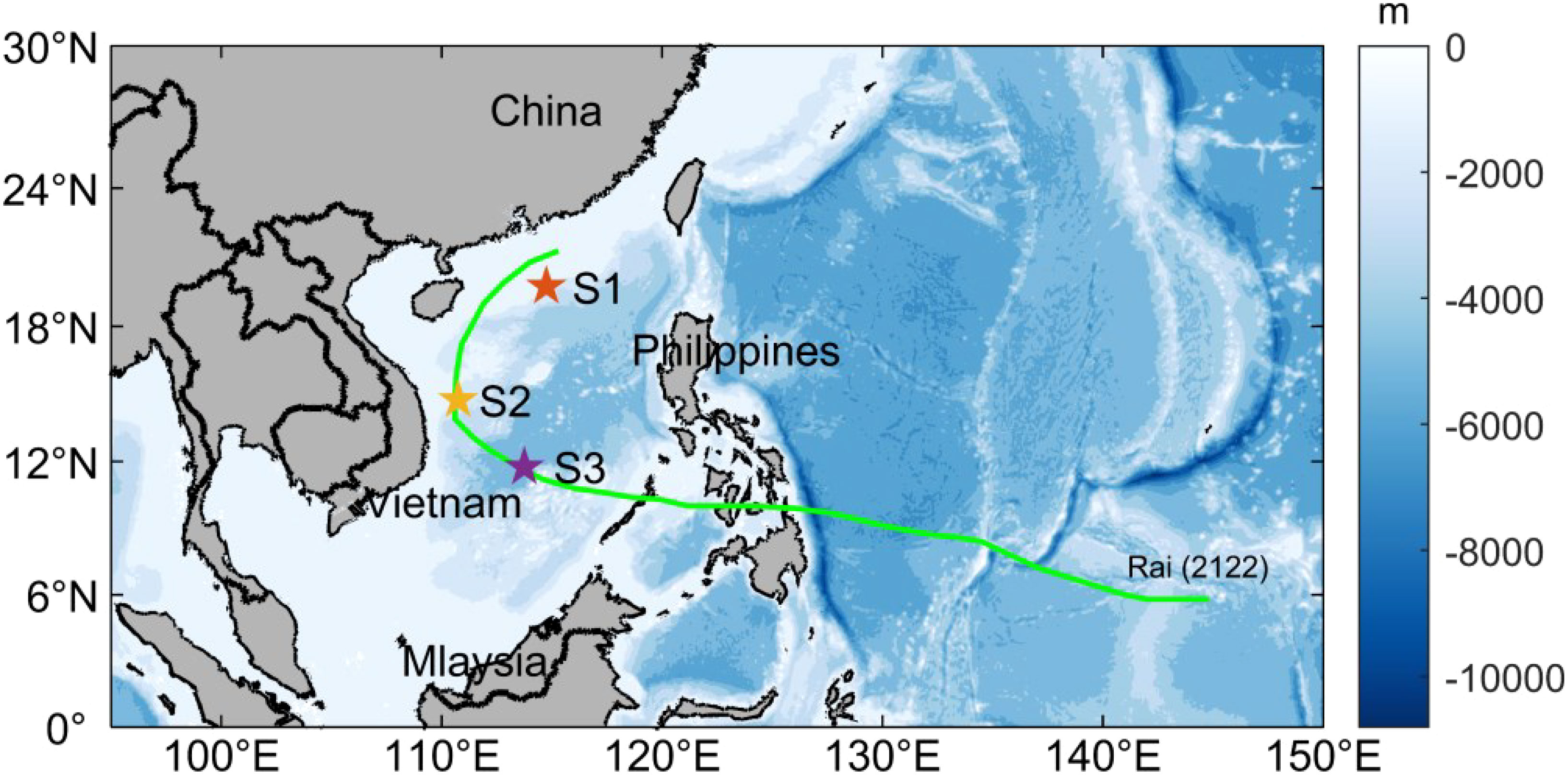
Figure 1 Location distribution of stations S1, S2, and S3, the green curve represents the path of Typhoon Rai.
2.2 Description of significant wave height prediction
For the SWH prediction of a certain station, it is essentially a time series prediction problem that takes past time series data as input and a certain amount of future time series data as output.
From the perspective of a time dimension, the observations at time length t form a tensor sequence X1, X2,…, Xt. Therefore, the SWH prediction problem can be defined as a tensor sequence of J time lengths in the past, to predict the tensor sequence of the next K time lengths:
In this study, we used the u10, v10, and SWH information of the three stations S1, S2, and S3 from 2018 to 2021 to predict SWH. Among them, we use the data from 2018-2020 as the training set and the data from 2021 as the validation set. To ensure the relative independence of training and validation data sets, the validation data is excluded from model training.
2.3 Methods
2.3.1 Recurrent neural network
RNN is a type of neural network for processing time series data. Figure 2 shows the RNN network structure. Compared with the traditional neural network whose inputs are independent of each other and cannot model sequence data with contextual relationships, RNN can retain the state of the previous input data. When the neuron calculates the current output, the previous neuron state is used as joint inputs are computed together. In this way, it has a great advantage in processing time series data.
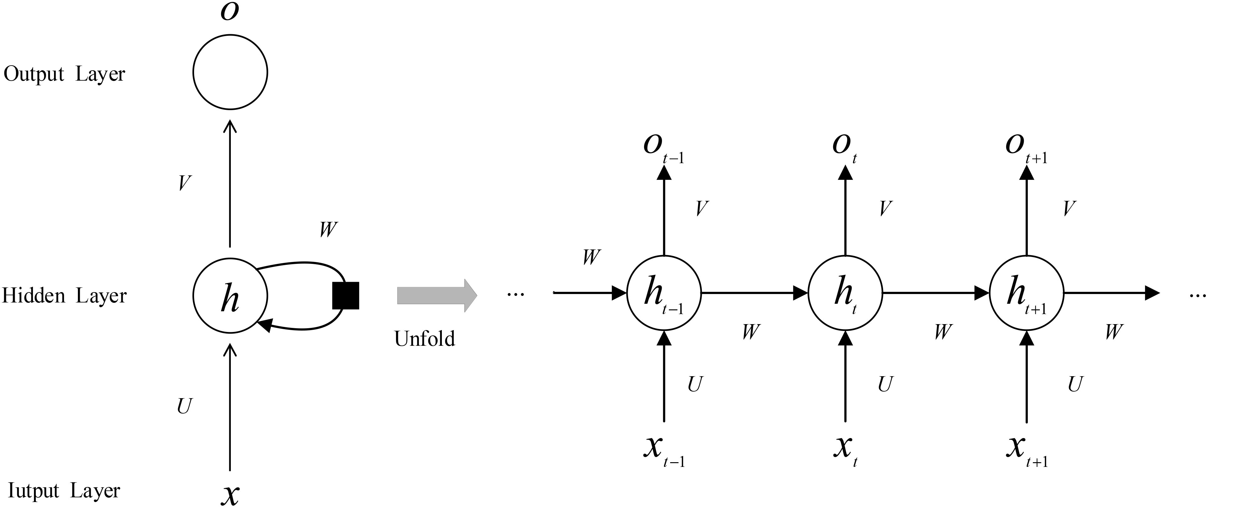
Figure 2 RNN module architecture.
The information state transfer formula of the unit at time t in RNN is as follows,
Where U is the weight matrix from the input layer to the hidden layer, ht is the state, ot is the output, bh and bo are the bias, W is the weight matrix from the state to the hidden layer, and V is the weight matrix from the hidden layer to the output layer. It can be seen from Figure 2 that the W, U, and V corresponding to each time node are unchanged. By this method, parameter sharing is achieved, and the number of parameters is greatly reduced.
2.3.2 Long short-term memory
LSTM is a special kind of RNN. As shown in Figure 3, LSTM uses two gates to control the content of the cell state c: one is the forget gate, which determines how much the unit state ct-1 from the previous moment is retained to the current moment ct; the other is the input gate, which determines how much of the input xt of the network at the current moment is saved in the unit state ct. The LSTM uses an output gate to control how much of the unit state ct is input to the current output value ht of the LSTM.
The information state transfer formula of the unit at time t in LSTM is as follows,
where ft represents the processing formula of the forget gate, it represents the processing formula of the input gate, zt is the unit state candidate vector at the current time, ot represents the processing formula of the output gate, W represents the given weight matrix, σ represents the sigmoid function, and · represents the element-wise product.
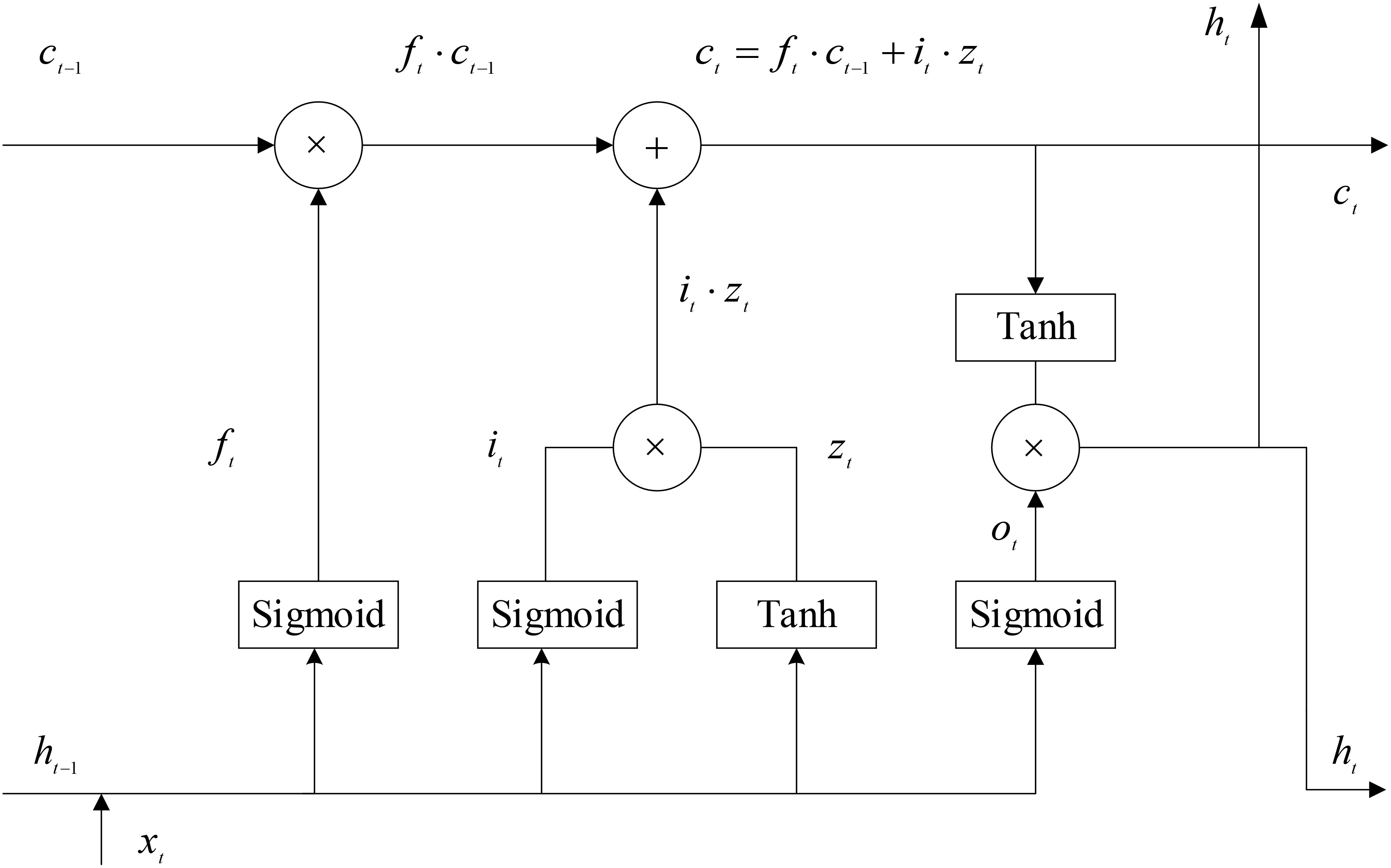
Figure 3 LSTM module architecture.
2.3.3 Gate recurrent unit
GRU is a variant of LSTM. GRU further simplifies the LSTM network, using only two gated structures, an update gate, and a reset gate, to update and transfer information. The update gate is responsible for controlling the influence of the state information of the previous moment on the state of the current moment. The larger the value of the update gate, the more the state information of the previous moment is brought in, and the reset gate is responsible for controlling the degree of ignoring the status information of the previous moment. The smaller the value of the reset gate, the more is ignored. Its unit structure is shown in Figure 4.

Figure 4 GRU module architecture.
The information state transfer formula of the unit at time t in GRU is as follows,
where zt is the processing formula of the update gate, rt is the processing formula of the reset gate, is the unit state candidate vector at the current time, ht is the output value, W represents the given weight matrix, σ represents the sigmoid function, and · represents the element-wise product.
2.4 Experimental design
2.4.1 Experimental environment
All models are trained using the Adam optimizer (Kingma and Ba, 2014) with a starting learning rate of 0.001. The training process is stopped after 30 epochs. All experiments are implemented in Pytorch (Paszke et al., 2019) and conducted on NVIDIA 3070 GPU. Other detailed parameter information in the experiment is listed in Table 1.
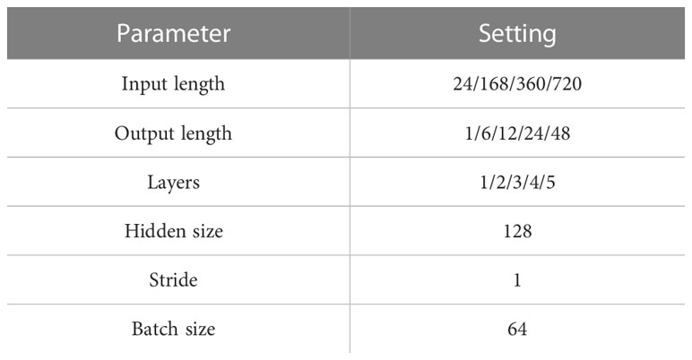
Table 1 Parameters setting.
2.4.2 Experimental procedures
In this study, all methods can achieve end-to-end training, and the entire calculation process does not require manual processing but is completely handed over to the deep learning model, from learning the input data feature to obtaining the result. The advantage of end-to-end training is that it reduces the complexity of computational processing. The overall flow of the experimental design is shown in Figure 5.

Figure 5 Experimental flow chart.
The detailed steps of the SWH prediction experiment are as follows.
(1) Data preprocessing, using the MinmaxScaler function of the sklearn library to normalize the input data.
(2) Divide the data, using the data from 2018-2020 as the training set and the data in 2021 as the validation set.
(3) Set a fixed random seed to ensure that each experiment can be reproduced.
(4) Model training, using the Mean Square Error (MSE) loss function and the Adam optimization function to iteratively train the model, and automatically save the optimal weight by recording the loss function value. During the training process, the learning rate is dynamically adjusted every 10 epochs to prevent the model from not converging.
(5) Visualization, visualize the experimental results and intuitively compare the SWH prediction ability of different methods.
2.4.3 Metrics
We use the following three measures to assess the model’s performance: Root Mean Square Error (RMSE), Mean Absolute Error (MAE), and Coefficient of Determination (R2). The following are the calculation algorithms for the above-mentioned three metrics,
where n is the total number of test samples, yi, and are the true value, the predicted value, and the arithmetic mean of yi, respectively. Note that the lower the RMSE and MAE values, the better the consistency between the measurement and the prediction, but the higher the R2 value, the more accurate the prediction.
3 Results
3.1 Effect of input length on SWH prediction performance
To verify the influence of the input length on the SWH prediction results, when the initial learning rate is 0.001, the number of hidden layers is 3, the hidden size is 128, and the prediction length is 24h, the input lengths are set to 24h, 168h, 360h, 720h, discuss the effect of input length on SWH prediction performance. The influence of input length on the prediction of SWH is shown in Table 2, in which the bold font is the optimal result of this group of experiments.

Table 2 The prediction result of significant wave height.
It can be seen from the experimental results that it is not that the longer the input length, the better the prediction effect. As the input length increases, the model’s SWH prediction performance tends to be poor. Although using the RNN model to predict SWH at S1, the best result is obtained when the input length is 168h, but from the overall trend, the SWH prediction effect still shows a downward trend. At S1, the prediction effect of RNN is the best, and the prediction effect of GRU is slightly better than that of LSTM. The possible reason is that the SWH of the S1 is lower throughout the year, and the complex model has the opposite effect. At S2 and S3, the GRU model had the best SWH prediction effect, and the values of RMSE and MAE were slightly higher than those at S1. The possible reason was that S1 and S2 had higher annual SWH and greater fluctuations. Overall, considering the SWH prediction performance of different models at S1, S2, and S3, when the input length is 24h, GRU predicts SWH the best, which also benefits from the unique design of the GRU model.
3.2 Effect of prediction length on SWH prediction performance
To verify the influence of prediction length on SWH prediction results, according to the analysis of experimental results in Section 3.1, the initial learning rate was set as 0.001, the number of hidden layers as 3, the hidden size as 128, the input length as 24h, and the output length as 1h, 6h, 12h, 24h, and 48h, respectively, to discuss the influence of output length on SWH prediction performance. The influence of prediction length on the prediction of SWH is shown in Table 3, in which the bold font is the optimal result of this group of experiments.
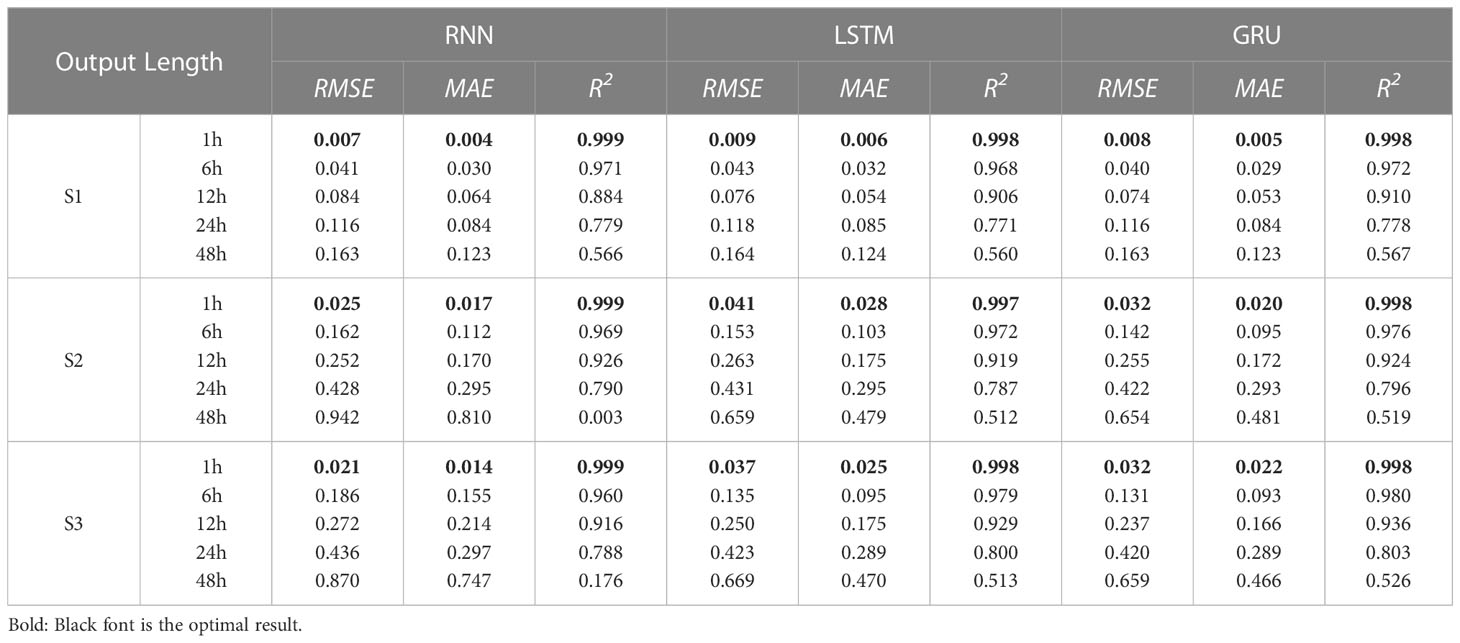
Table 3 The prediction result of significant wave height.
It can be seen from the results that with the increase in the prediction length, the prediction effect gradually decreases. In S1, S2, and S3, the prediction results of the RNN method in 1h are all the best, the possible reason is that the RNN model is relatively simple and the prediction length is short. However, the prediction results at 48h show that the SWH prediction effect of the RNN model is poor and may not be used for long-term SWH prediction. As the prediction length increases, the advantages of the unique design of the LSTM and GRU models emerge. Overall, the SWH prediction performance of the GRU model is slightly better than that of the LSTM model. The RNN model has certain advantages in short-term SWH prediction, but as the prediction length gradually increases to 24h later, it loses its effect.
3.3 Effect of hidden layers on SWH prediction performance
To verify the influence of the hidden layers on the SWH prediction results, when the initial learning rate is 0.001, the hidden size is 128, the input length is 24h, and the prediction length is 24h, discuss the effect of layers on SWH prediction performance. The influence of hidden layers on the prediction of SWH is shown in Table 4, in which the bold font is the optimal result of this group of experiments.
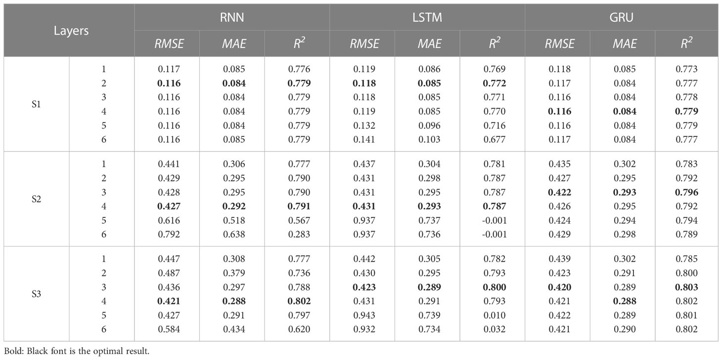
Table 4 The prediction result of significant wave height.
It can be seen from the results that it is not that the more layers of the model, the better the prediction performance. In S1, RNN and LSTM have the best SWH prediction performance when the number of layers is set to 2, but GRU can also achieve the same prediction performance when the number of layers is set to 4. In S2, RNN and LSTM have the best SWH prediction performance when the number of layers is set to 4, and the SWH prediction performance of RNN is slightly better than that of LSTM; GRU can achieve the best SWH performance when the number of layers is set to 3 and is better than RNN, LSTM. In S3, the prediction effect of GRU is the best when the number of layers is set to 3. To sum up, when building a model to predict SWH, it is necessary to set a reasonable number of layers, to achieve the goal of low calculation amount and good prediction effect.
3.4 Experiments on typhoon cases to test the performance of SWH prediction
Typhoon Rai (No. 2122) formed on December 13, 2021, in the low latitudes of the Northwest Pacific Ocean. It developed slowly at the beginning, and then experienced rapid intensification twice in the coastal waters east of the Philippines and after crossing the Philippines and entering the South China Sea, reaching the level of a super typhoon identified by the Central Meteorological Observatory. On December 21, it gradually weakened and dissipated. Typhoon “Rai” became the strongest super typhoon affecting the South China Sea since meteorological records began.
To better study the prediction ability of SWH under extreme environments, we selected the period from December 1, 2021, to December 31, 2021, at S1, S2, and S3 for the experiment. When the initial learning rate is 0.001, the hidden size is 128, the number of layers is 3, the input length is 24h, and the prediction length is 1h, 6h, 12h, and 24h respectively, we comprehensively analyze the advantages and disadvantages of SWH prediction by different methods in the extreme environment by analyzing the prediction and real comparison curve and the error value curve.
It can be seen from Figure 6 that the three methods of RNN, LSTM, and GRU all showed better prediction performance in the 1h short-term SWH prediction. Specifically, at the peak of SWH, the RNN method can fit well, while LSTM and GRU will predict too high or too low. In this respect, the SWH prediction effect of RNN is slightly better than that of LSTM and GRU. As the prediction time increases, the prediction performance of the three methods starts to decrease. It can be seen from Figure 7 that during the 6h SWH prediction process, in S1, the prediction of LSTM at the peak is greater than the actual value. In S2, a similar situation also occurs, but this situation does not exist in S3. The possible reason is data features that lack similar variation features in the training set. As can be seen from Figure 8, in the 12h SWH prediction, LSTM still has the situation mentioned above. We have reason to think that this is caused by the lack of data with similar changing characteristics in the training set. With the further increase of the forecast time, it can be seen from Figure 9 that the SWH prediction results of the three methods are compared with the true value, and the 24h prediction results have an obvious trend of lagging, and there will be a certain prediction error at the peak. However, the overall trend is still roughly the same, indicating that RNN, LSTM, and GRU still have certain reference values for the prediction of long-term SWH in extreme environments.
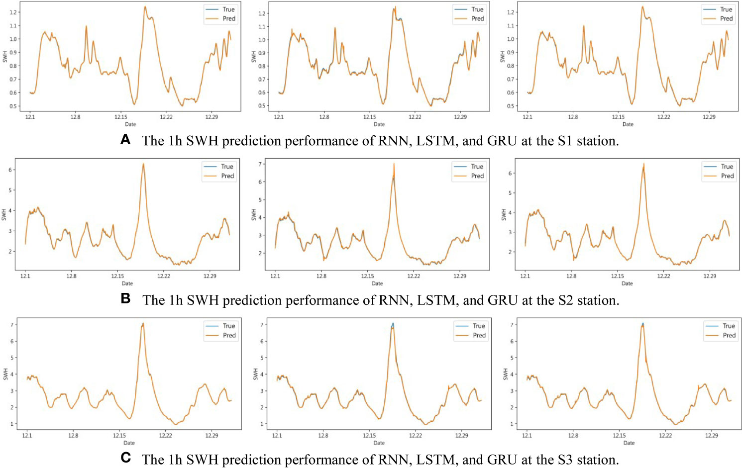
Figure 6 1h SWH prediction performance of RNN, LSTM, and GRU at S1, S2, and S3. (A) The 1h SWH prediction performance of RNN, LSTM, and GRU at the S1 station. (B) The 1h SWH prediction performance of RNN, LSTM, and GRU at the S2 station. (C) The 1h SWH prediction performance of RNN, LSTM, and GRU at the S3 station.
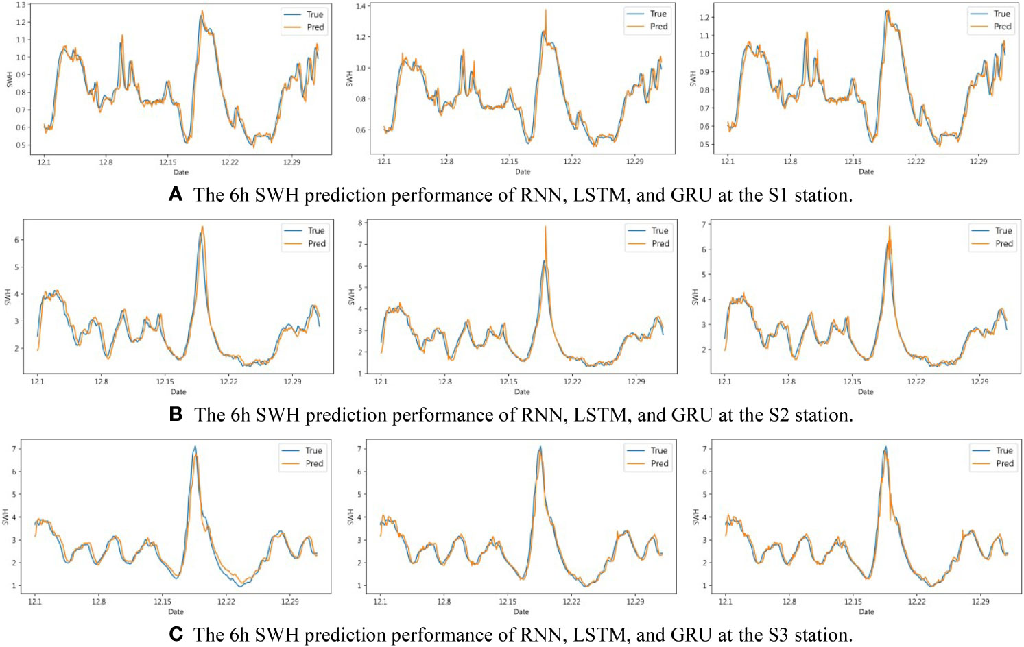
Figure 7 6h SWH prediction performance of RNN, LSTM, and GRU at S1, S2, and S3. (A) The 6h SWH prediction performance of RNN, LSTM, and GRU at the S1 station. (B) The 6h SWH prediction performance of RNN, LSTM, and GRU at the S2 station. (C) The 6h SWH prediction performance of RNN, LSTM, and GRU at the S3 station.
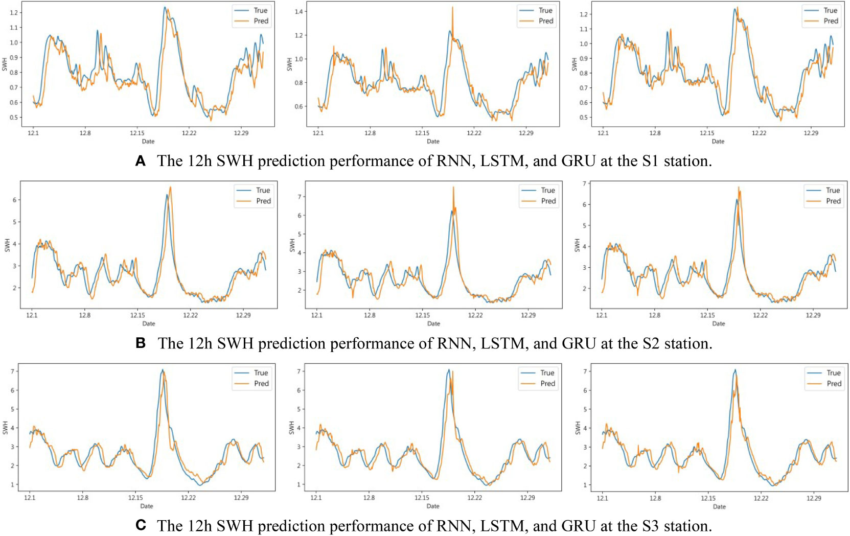
Figure 8 12h SWH prediction performance of RNN, LSTM, and GRU at S1, S2, and S3. (A) The 12h SWH prediction performance of RNN, LSTM, and GRU at the S1 station. (B) The 12h SWH prediction performance of RNN, LSTM, and GRU at the S2 station. (C) The 12h SWH prediction performance of RNN, LSTM, and GRU at the S3 station.

Figure 9 24h SWH prediction performance of RNN, LSTM, and GRU at S1, S2, and S3. (A) The 24h SWH prediction performance of RNN, LSTM, and GRU at the S1 station. (B) The 24h SWH prediction performance of RNN, LSTM, and GRU at the S2 station. (C) The 24h SWH prediction performance of RNN, LSTM, and GRU at the S3 station.
4 Conclusions
Predicting SWH is conducive to understanding the sea wave conditions in advance, effectively improving the safety of marine activities, and reducing the occurrence of marine accidents, which is of great significance to the development of national security and the marine economy. This paper comprehensively analyzes and discusses the SWH prediction performance of RNN, LSTM, and GRU. The main findings of this paper are as follows:
(1) The input length has an influence on the prediction results, but it does not mean that the longer the input length, the better the prediction performance. As the input length increases, the SWH prediction performance of the model tends to decrease.
(2) The prediction length has an influence on the prediction results. As the prediction length increases, the prediction performance gradually decreases. But in the 48h SWH prediction, the prediction performance of RNN is the worst, which is not suitable for long-term SWH prediction.
(3) The more layers of the model, the better the SWH prediction performance is not necessarily. When establishing an SWH prediction model, it is necessary to set the number of layers reasonably to achieve the purpose of less calculation and better prediction performance.
Deep learning methods have achieved good results in predicting SWH experiments. But there are also certain defects: (1) It is like a “black box”. The inference mechanism between input and output is unclear. (2) These methods focus on time series research the response to spatial changes is not obvious. In future work, we will focus on the interpretability of the model and generalize the research scope from a single point to a region.
Data availability statement
The original contributions presented in the study are included in the article/supplementary material. Further inquiries can be directed to the corresponding author.
Author contributions
PH designed the experiment. YG collected and analyzed the data. SL provided a critical revision of the article. All authors contributed to the article and approved the submitted version.
Funding
This work was supported by the National Natural Science Foundation of China (Grant Number 41876003).
Acknowledgments
We would like to acknowledge the organizations that provided the sources of the data used in this work - namely, the European Centre for Medium-Range Weather Forecasts. We also thank the HPC Center of Zhejiang University (Zhoushan Campus) for computational support.
Conflict of interest
The authors declare that the research was conducted in the absence of any commercial or financial relationships that could be construed as a potential conflict of interest.
Publisher’s note
All claims expressed in this article are solely those of the authors and do not necessarily represent those of their affiliated organizations, or those of the publisher, the editors and the reviewers. Any product that may be evaluated in this article, or claim that may be made by its manufacturer, is not guaranteed or endorsed by the publisher.
References
Berbić J., Ocvirk E., Carević D., Lončar G. (2017). Application of neural networks and support vector machine for significant wave height prediction. Oceanologia 59 (3), 331–349. doi: 10.1016/j.oceano.2017.03.007
Bethel B. J., Sun W., Dong C., Wang D. (2022). Forecasting hurricane-forced significant wave heights using a long short-term memory network in the Caribbean Sea. Ocean Sci. 18 (2), 419–436. doi: 10.5194/os-18-419-2022
Callens A., Morichon D., Abadie S., Delpey M., Liquet B. (2020). Using random forest and gradient boosting trees to improve wave forecast at a specific location. Appl. Ocean Res. 104, 102339. doi: 10.1016/j.apor.2020.102339
Chen X., Huang W. (2021). Spatial–temporal convolutional gated recurrent unit network for significant wave height estimation from shipborne marine radar data. IEEE Trans. Geosci. Remote Sens. 60, 1–11. doi: 10.1109/TGRS.2020.3034752
Deshmukh A. N., Deo M. C., Bhaskaran P. K., Nair T. M. B., Sandhya K. G. (2016). Neural-Network-Based data assimilation to improve numerical ocean wave forecast. IEEE J. Ocean. Eng. 41 (4), 944–953. doi: 10.1109/joe.2016.2521222
Dey R., Salem F. M. (2017). “Gate-variants of gated recurrent unit (GRU) neural networks,” in 2017 IEEE 60th international midwest symposium on circuits and systems (MWSCAS). 1597–1600 (IEEE).
Emmanouil S., Aguilar S. G., Nane G. F., Schouten J.-J. (2020). Statistical models for improving significant wave height predictions in offshore operations. Ocean Eng. 206, 107249. doi: 10.1016/j.oceaneng.2020.107249
Fan S., Xiao N., Dong S. (2020). A novel model to predict significant wave height based on long short-term memory network. Ocean Eng. 205, 107298. doi: 10.1016/j.oceaneng.2020.107298
Gao S., Huang J., Li Y., Liu G., Bi F., Bai Z. (2021b). A forecasting model for wave heights based on a long short-term memory neural network. Acta Oceanol. Sin. 40 (1), 62–69. doi: 10.1007/s13131-020-1680-3
Gao D., Liu Y., Meng J., Jia Y., Fan C. (2018). Estimating significant wave height from SAR imagery based on an SVM regression model. Acta Oceanol. Sin. 37 (3), 103–110. doi: 10.1007/s13131-018-1203-7
Gao J., Ma X., Dong G., Chen H., Liu Q., Zang J. (2021a). Investigation on the effects of Bragg reflection on harbor oscillations. Coast. Eng. 170, 103977. doi: 10.1016/j.coastaleng.2021.103977
Gao J., Ma X., Zang J., Dong G., Ma X., Zhu Y., et al. (2020). Numerical investigation of harbor oscillations induced by focused transient wave groups. Coast. Eng. 158, 103670. doi: 10.1016/j.coastaleng.2020.103670
Gopinath D. I., Dwarakish G. S. (2016). Real-time prediction of waves using neural networks trained by particle swarm optimization. Int. J. Ocean Climate Syst. 7 (2), 70–79. doi: 10.1177/1759313116642896
Group T. W. (1988). The WAM model–a third generation ocean wave prediction model. J. Phys. Oceanogr. 18 (12), 1775–1810. doi: 10.1175/1520-0485(1988)018<1775:TWMTGO>2.0.CO;2
Huang W., Dong S. (2021). Improved short-term prediction of significant wave height by decomposing deterministic and stochastic components. Renewable Energy 177, 743–758. doi: 10.1016/j.renene.2021.06.008
Jörges C., Berkenbrink C., Stumpe B. (2021). Prediction and reconstruction of ocean wave heights based on bathymetric data using LSTM neural networks. Ocean Eng. 232, 109046. doi: 10.1016/j.oceaneng.2021.109046
Kazeminezhad M. H., Siadatmousavi S. M. (2017). Performance evaluation of WAVEWATCH III model in the Persian gulf using different wind resources. Ocean Dyn. 67 (7), 839–855. doi: 10.1007/s10236-017-1063-2
Kingma D. P., Ba J. (2014). Adam: A method for stochastic optimization. arXiv preprint arXiv 1412, 6980.
Liang B., Gao H., Shao Z. (2019). Characteristics of global waves based on the third-generation wave model SWAN. Mar. Structures 64, 35–53. doi: 10.1016/j.marstruc.2018.10.011
Li N., Cheung K. F., Cross P. (2020). Numerical wave modeling for operational and survival analyses of wave energy converters at the US navy wave energy test site in Hawaii. Renewable Energy 161, 240–256. doi: 10.1016/j.renene.2020.06.089
Li S., Hao P., Yu C., Wu G. (2021). CLTS-net: A more accurate and universal method for the long-term prediction of significant wave height. J. Mar. Sci. Eng. 9 (12), 1464. doi: 10.3390/jmse9121464
Liu Q., Rogers W. E., Babanin A. V., Young I. R., Romero L., Zieger S., et al. (2019). Observation-based source terms in the third-generation wave model WAVEWATCH III: Updates and verification. J. Phys. Oceanogr. 49 (2), 489–517. doi: 10.1175/jpo-d-18-0137.1
Miky Y., Kaloop M. R., Elnabwy M. T., Baik A., Alshouny A. (2021). A recurrent-Cascade-Neural network- nonlinear autoregressive networks with exogenous inputs (NARX) approach for long-term time-series prediction of wave height based on wave characteristics measurements. Ocean Eng. 240, 109958. doi: 10.1016/j.oceaneng.2021.109958
Ni C., Ma X. (2020). An integrated long-short term memory algorithm for predicting polar westerlies wave height. Ocean Eng. 215, 107715. doi: 10.1016/j.oceaneng.2020.107715
Paszke A., Gross S., Massa F., Lerer A., Bradbury J., Chanan G., et al. (2019). “Pytorch: An imperative style, high-performance deep learning library,” in Advances in neural information processing systems, 32.
Peres D. J., Iuppa C., Cavallaro L., Cancelliere A., Foti E. (2015). Significant wave height record extension by neural networks and reanalysis wind data. Ocean Model. 94, 128–140. doi: 10.1016/j.ocemod.2015.08.002
Sadeghifar T., Nouri Motlagh M., Torabi Azad M., Mohammad Mahdizadeh M. (2017). Coastal wave height prediction using recurrent neural networks (RNNs) in the south Caspian Sea. Mar. Geodesy 40 (6), 454–465. doi: 10.1080/01490419.2017.1359220
Swain J., Umesh P., Balchand A. (2019). WAM and WAVEWATCH-III intercomparison studies in the north Indian ocean using oceansat-2 scatterometer winds. J. Ocean Climate 9, 2516019219866569. doi: 10.1177/2516019219866569
Umesh P. A., Swain J. (2018). Inter-comparisons of SWAN hindcasts using boundary conditions from WAM and WWIII for northwest and northeast coasts of India. Ocean Eng. 156, 523–549. doi: 10.1016/j.oceaneng.2018.03.029
Vanem E. (2016). Joint statistical models for significant wave height and wave period in a changing climate. Mar. Structures 49, 180–205. doi: 10.1016/j.marstruc.2016.06.001
Wang D.-P., Oey L.-Y. (2008). Hindcast of waves and currents in hurricane Katrina. Bull. Am. Meteorol. Soc. 89 (4), 487–496. doi: 10.1175/BAMS-89-4-487
Young I. R., Ribal A. (2019). Multiplatform evaluation of global trends in wind speed and wave height. Science 364 (6440), 548–552. doi: 10.1126/science.aav9527
Yu Y., Si X., Hu C., Zhang J. (2019). A review of recurrent neural networks: LSTM cells and network architectures. Neural Comput. 31 (7), 1235–1270. doi: 10.1162/neco_a_01199
Zaremba W., Sutskever I., Vinyals O. (2014). Recurrent neural network regularization. arXiv preprint arXiv 2329 (2014), 1409.
Zhang X., Li Y., Gao S., Ren P. (2021). Ocean wave height series prediction with numerical long short-term memory. J. Mar. Sci. Eng. 9 (5), 514. doi: 10.3390/jmse9050514
Keywords: significant wave height, South China Sea, deep learning, RNN, LSTM, GRU
Citation: Hao P, Li S and Gao Y (2023) Significant wave height prediction based on deep learning in the South China Sea. Front. Mar. Sci. 9:1113788. doi: 10.3389/fmars.2022.1113788
Received: 01 December 2022; Accepted: 21 December 2022;
Published: 23 February 2023.
Edited by:
Lichuan Wu, Uppsala University, SwedenReviewed by:
Carlos Pérez-Collazo, University of Vigo, SpainJunliang Gao, Jiangsu University of Science and Technology, China
Copyright © 2023 Hao, Li and Gao. This is an open-access article distributed under the terms of the Creative Commons Attribution License (CC BY). The use, distribution or reproduction in other forums is permitted, provided the original author(s) and the copyright owner(s) are credited and that the original publication in this journal is cited, in accordance with accepted academic practice. No use, distribution or reproduction is permitted which does not comply with these terms.
*Correspondence: Shuang Li, bHNodWFuZ0B6anUuZWR1LmNu