USFP: An unbalanced severe typhoon formation prediction framework based on transfer learning

Introduction: Severe typhoons, as extreme weather events, can cause a large number of casualties and property damage in coastal areas. There are mainly three kinds of methods for the prediction of severe typhoon formation, which are the numerical-based methods, the statistical-based methods, and the machine learning-based methods. However, existing methods do not consider the unbalance between the number of ordinary typhoon samples and severe typhoon samples, which makes the accuracies of existing methods in the prediction of severe typhoons much lower than that of ordinary typhoons.

Methods: In this paper, we propose an unbalanced severe typhoon formation prediction (USFP) framework based on transfer learning. We first propose a severe typhoon pre-learning model which is used to learn prior knowledge from a constructed balanced dataset. Then, we propose an unbalanced severe typhoon re-learning model which utilizes the prior knowledge learning from the pre-learning model. Our USFP framework fuses three different variables, which are atmospheric variables, sea surface variables, and ocean hydrographic variables.

Results: Extensive experiments based on datasets of three different regions show that our USFP framework outperforms the numerical model IFS of ECMWF and existing machine learning methods.

1 Introduction

A tropical cyclone (TC) is a powerful and profound tropical weather system. As extreme weather, severe typhoons not only cause great economic damage to coastal areas but also greatly endanger people’s lives and property. According to statistics from the National Meteorological Administration of China, in 2018, about 32 million people were affected by typhoons, and the direct economic loss reached 69.73 billion RMB (China Meteorological Administration, 2020). Severe typhoons, which are more powerful than ordinary typhoons, bring more serious disasters.

In recent years, machine learning-based methods have been widely used in meteorology and oceanography. (Mecikalski et al., 2021; Wikner et al., 2021; Fei et al., 2022). Tropical cyclones (including severe typhoons) are a high-impact and disastrous weather phenomenon in meteorology and oceanography. There are mainly three kinds of methods used to predict the formation of tropical cyclones: the numerical-based methods, the statistical-based methods, and the machine learning-based methods. First, the typical numerical-based methods are the hurricane weather research forecast model (HWRF), the Global Forecast System (GFS), and the Integrated Forecasting System (IFS), which are used to forecast future weather by numerically solving a set of hydrodynamic and thermodynamic equations and the main forecasting method used by many official organizations in the world (John, 2019). Second, the typical statistical-based methods of TC prediction are the Statistical Typhoon Intensity Prediction Scheme (STIPS) and the Statistical Hurricane Intensity Prediction Scheme (SHIPS), which are based on the numerical-based methods to build forecasting models considering future changes in the atmospheric and oceanic conditions. The third is the machine learning-based methods, which are data-driven methods that do not consider physical mechanisms. Meteorologists apply machine learning models such as AdaBoost Algorithm (Zhang et al., 2019), SVM (Richman et al., 2017; Kim et al., 2019), CNN (Matsuoka et al., 2018), and Fuzzy Neural Network (Yip and Yau, 2011) to tropical cyclone prediction. However, existing studies do not consider the unbalanced characteristics of the typhoon samples. The number of samples between ordinary typhoons and severe typhoons is quite different as shown in Table 1. This makes the prediction accuracy of severe typhoons will be decreased.

TABLE 1

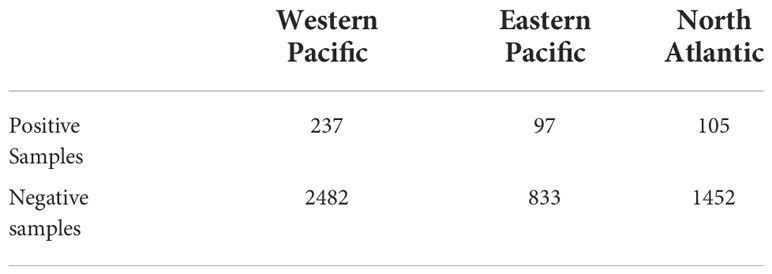
Table 1 The number of positive and negative samples in different regions counted from the World Meteorological Organization (WMO) version of the International Best Trajectory Archive for Climate Management (IBTrACS) Global Tropical Cyclone Best Trajectory Dataset.

In this paper, we propose an unbalanced severe typhoon formation prediction (USFP) framework, which is based on the transfer learning method (Yosinski et al., 2014; Long et al., 2015). Our USFP framework can effectively minimize the impact of unbalanced data on severe typhoon formation prediction. It first learns prior knowledge from a balanced dataset extracted from the unbalanced dataset with the severe typhoon pre-learning model shown in Section 4.2. Then, the prior knowledge is transferred to the unbalanced severe typhoon re-learning model for training as described in Section 4.3. Our USFP framework fuses three variables: atmospheric variables, sea surface variables, and ocean hydrographic variables. Extensive experiments in three different regions show that our USFP framework outperforms the numerical model IFS of ECMWF and existing machine learning methods.

Contributions of this paper include:

1. We propose an unbalanced severe typhoon formation prediction (USFP) framework based on transfer learning. The USFP framework is trained by transferring prior knowledge obtained from a balanced dataset to the unbalanced severe typhoon re-learning model. To the best of our knowledge, we are the first to use transfer learning to improve the prediction accuracies of severe typhoons.

2. We design a customized loss function to optimize our USFP framework, which assigns different weights to different categories of ordinary typhoon samples and severe typhoon samples.

3. We fuse multiple data from atmospheric variables, sea surface variables, and ocean hydrographic variables to predict severe typhoon formation. Extensive experiments performed on data from three regions show that our USFP framework can effectively improve the forecasting effect of unbalanced severe typhoon formation.

The rest of this paper is organized as follows: Section 2 reviews the current studies in the field; Section 3 defines the unbalanced severe typhoon problem in this paper; Section 4 describes the structure of the USFP framework; Section 5 demonstrates the effectiveness of the USFP framework through experiments; Section 6 summarizes the current work in this paper and gives an outlook on future work.

2 Related work

At present, there is a lack of research on the formation of unbalanced severe typhoons. Therefore, this section reviews research in the field of tropical cyclone forecasting and data unbalance, which is used to explore methods to solve the problem of unbalanced severe typhoon formation prediction.

2.1 Tropical cyclone forecasting

2.1.1 Numerical-based methods

The numerical-based methods forecast the environmental field through the meteorological marine environmental conditions and then extrapolate the forecast of typhoon elements, which is done through model initialization and physical process parameterization. At present, the numerical-based methods have an accuracy rate of 70-80% (Halperin et al., 2013) and are used in many official organizations like the hurricane weather research forecast model (HWRF), the Global Forecast System (GFS), and the Integrated Forecasting System (IFS) of the European Centre for Medium-Range Weather Forecast (ECMWF). For example, Elsberry et al. (2021) improved the Pacific typhoon intensity prediction technology based on ECMWF and successfully predicted the rapid intensification events after the formation of tropical cyclones. Na et al. (2018) evaluated the intensity forecast error of tropical cyclones and the analysis found that the official is more mature in predicting the weakening problem than the intensification problem. The numerical-based methods have had a lot of fruitful research work in typhoon physical law perception and forecasting. However, the numerical-based methods have shortcomings such as incomplete expression of complex physical processes, low accuracy of typhoon intensity prediction, and high computational cost.

2.1.2 Statistical-based methods

The statistical-based methods are based on numerical weather forecasts and take into account changes in the future atmospheric environment and ocean conditions to build forecast models. The method achieves the prediction of TC by analyzing the regularity of a large amount of data and representing it with a functional relationship equation. Some of the typical methods are the Statistical Typhoon Intensity Prediction Scheme (STIPS) (Demaria and Kaplan, 1994) and the Statistical Hurricane Intensity Prediction Scheme (SHIPS) (Fritsch and Chappell, 1980; DeMaria and Kaplan, 1999; Knaff et al., 2005). The STIPS is a multiple linear regression model based on a statistical-dynamical framework, which is constructed by using a large amount of environmental information obtained from the Navy Operational Global Analysis and Prediction System (NOGAPS). The SHIPS is commonly used in the Atlantic and East Pacific regions, which has good results in tropical cyclone forecasting. The regression coefficients of the SHIPS are updated each year after the hurricane season with the latest samples and improved operational forecasting. The statistical-based methods have been relatively well applied in TC intensity prediction. However, because the statistical-based methods are often helpless in the face of massive data, it is difficult to extract critical and effective forecast information.

2.1.3 Machine learning-based methods

In recent years, machine learning has achieved good results in numerous fields. Therefore, many scholars have applied it to the field of tropical cyclones forecasting. These methods compensate for the shortcomings of the statistical-based methods and the numerical-based methods to some extent. For example, Wijnands et al. (2016) of the University of Melbourne, Australia, used the Peter Clark algorithm to select the best predictors for short-term formation forecasts of tropical cyclones. Zhang et al. (2015) of Brookhaven National Laboratory in the United States tried to use nonlinear ensemble machine learning classifiers to determine whether a mesoscale convective system would evolve into a tropical cyclone in different prediction periods. Ahijevych et al. (2016) of the National Center for Atmospheric Research in the United States used the random forest algorithm to predict the possibility of a mesoscale convective system developing into a tropical cyclone within 2 hours. Based on WindSat satellite ocean surface wind and precipitation data, Park et al. (2016) from the Busan Institute of Ocean Science and Technology in South Korea used decision trees to analyze the intensity of tropical cyclones. Higa et al. (2021) successfully estimated typhoon intensity with high accuracy by using the VGG-16 model to process a single satellite image and combining the knowledge of the meteorological domain. The machine learning-based methods as data-driven methods can ignore the imprecise physical mechanisms of typhoon formation and have significant advantages in capturing the nonlinear relationship between forecast factors and forecast targets (Reichstein et al., 2019).

2.2 Unbalanced data problems

2.2.1 Data sampling-based methods

The data sampling-based methods are to manually balance the unbalanced datasets by over-sampling or under-sampling, which are widely used to solve unbalanced problems in the field of machine learning. Han et al. (2005) designed an improved oversampling algorithm based on the SMOTE algorithm, which only uses the minority class samples on the boundary to synthesize new samples, thereby improving the class distribution of the samples. Yan and Cao (2019) proposed two feature-based oversampling methods to rebalance binary and multi-class time series datasets with good results in terms of statistical significance. In contrast, Liu et al. (2009) used an ensemble learning mechanism to optimize the traditional undersampling method with a better training effect. an ensemble learning-based undersampling technique. However, the data sampling-based methods such as oversampling and undersampling cannot meet the requirement of the actual forecast of severe typhoons and are not suitable for solving the problems faced in this paper.

2.2.2 Algorithm improvement-based methods

The core idea of the algorithm improvement-based methods is to make the model more focused on the sample size less class as a way to improve the prediction accuracy of small sample data. For example, Mo et al. (2019) proposed an unbalanced sample classification algorithm based on the deep residual network, which has a recognition rate close to 100% for small sample unbalanced datasets. Hu et al. (2018) proposed a multi-task learning framework using an attribute attention mechanism to capture key information and improved the accuracy of crime charge prediction for small samples. Cui et al. (2019) designed a weight adjustment scheme to rebalance the loss using the effective number of samples per class, which resulted in a class-balanced loss that can achieve significant performance gains on long-tailed datasets. Geng and Luo (2019) modified the standard CNN to a cost-sensitive network (CS-CNN), which can use the category-dependent cost matrix to penalize misclassified samples. Zhan (2020) used the loss function of Focal loss (Lin et al., 2017) to establish a network model based on the DNN-LSTM, which had a better result for the problem of unbalanced data.

2.2.3 Transfer learning-based methods

The transfer learning-based approach is to use the pre-trained model parameters for the training of new models, which helps to improve the accuracy of samples with fewer data in the dataset. Taherkhani et al. (2020) proposed the AdaBoost-CNN model based on transfer learning with 16.98% higher accuracy compared to the classical Adaboost. Al-Stouhi and Reddy (2016) proposed a Rare-Transfer transfer learning algorithm with a label-dependent update mechanism that can effectively handle rare class classification problems. Troncoso et al. (2018) transformed the problem of predicting extreme monsoons into an unbalanced binary classification problem and performed transfer learning on a series of related technical models. Singh et al. (2020) used VGG-19 as the base model and supplemented it with several techniques to achieve better results than existing frameworks. Lee et al. (2016) used a CNN classifier model based on transfer learning to normalize the data by thresholding the large-class data and obtained better results on small classes of data.

Transfer learning is not only applied to the problem of imbalanced data, some researchers have also applied transfer learning to the prediction of tropical cyclones. Deo et al. (2017) assessed the relationship between different types of cyclones by using transfer learning and traditional neural network methods to achieve more stable intensity predictions for tropical cyclones. Pang et al. (2021) combined a deep convolutional generative adversarial network (DCGAN) and the YOLOv3 model to propose a New Detection Framework of Tropical Cyclones (NDFTC) with good stability and accuracy. Combinido et al. (2018). used a Visual GeometrCombinidoy Group 19-1ayer CNN (VGG19) model to estimate TC intensity on TC grayscale infrared images obtained from various geostationary satellites, which achieved lower RMSE. The transfer learning-based methods can improve the focus on the minority class while maintaining the classification accuracy of the majority class. When forecasting the formation of severe typhoons, it is necessary to focus on the accuracy of forecasting the formation of severe typhoons but the forecast accuracy of non-severe typhoons cannot be ignored. Therefore, we use the idea of transfer learning to build the USFP framework to solve the problem of unbalanced severe typhoon formation.

3 Problem definitions

The formation of typhoons requires a combination of both atmospheric and oceanic factors. To simulate the atmospheric and oceanic factors of typhoon formation, we convert the variables into multidimensional tensors. Since the atmospheric variables and ocean hydrographic variables are in a 3D space, the atmospheric environment field corresponding to a typhoon can be represented as L×W×H×A three-dimensional grid data, where L and W represent longitude and latitude, H represents the height of the atmosphere and A represents atmospheric environment variables. Similarly, the ocean hydrographic environment field corresponding to a typhoon can be represented as L×W×D×R three-dimensional grid data, where D represents the depth of the ocean and R represents ocean hydrographic variables. And since the sea surface variables are in a 2D space. The sea surface environment field corresponding to a typhoon can be represented as a L×W×O two-dimensional grid data, where L and W represent longitude and latitude and O represents sea surface variables. The prediction variables including the atmosphere, sea surface and ocean hydrography can be represented by X=[ X^P,X^S,X^O] . Since the above spatial environment variables are time dependent, our problem can be regarded as a spatio-temporal prediction problem to predict whether a strong typhoon will form or not. Given typhoon spatio-temporal data: X=x_t−6b (b=0,1,⋯,t/6 ), the predicted typhoon state can be defined as:

$\begin{array}{ll}\begin{array}{c}{Y}_{t+6k}=f\left(x_t,x_{t-6},\cdots ,x_{t-6b}\right),k=1,2,3\cdots ,b=0,1,2\cdots \end{array}& (1)\end{array}$

where t is the prediction moment, X_t represents the atmospheric, sea surface, and ocean hydrographic variables at the prediction moment, Y_t+6k represents the predicted typhoon state, k represents the timestep of the prediction and b represents the lookback step before the prediction moment. We consider typhoons with wind speed reaching 84 kt as strong typhoons, which are positive samples. The rest of the typhoons are as non-strong typhoons, which are negative samples. When Y_t+6k=1 , it means that a severe typhoon is formed, which is a positive sample. When Y_t+6k=0 , it means that a severe typhoon is not formed, which is a negative sample. However, according to the defined standard, the number of positive and negative samples obtained is very unbalanced as shown in Table 1. Therefore, the severe typhoon formation prediction problem can be regarded as an unbalanced spatio-temporal series binary classification problem.

4 Methods

This section presents the details of the unbalanced severe typhoon formation prediction (USFP) framework. The first subsection introduces the overall architecture of the framework and the training method of the framework. The second subsection introduces the main structure of the severe typhoon pre-learning model. The last subsection details the structure of the unbalanced severe typhoon re-learning model and the loss function designed for it.

4.1 Architecture

The overall framework is shown in Figure 1. As we can see, the framework consists of two parts: the first part is the severe typhoon pre-learning model and the second part is the unbalanced severe typhoon re-learning model.

FIGURE 1

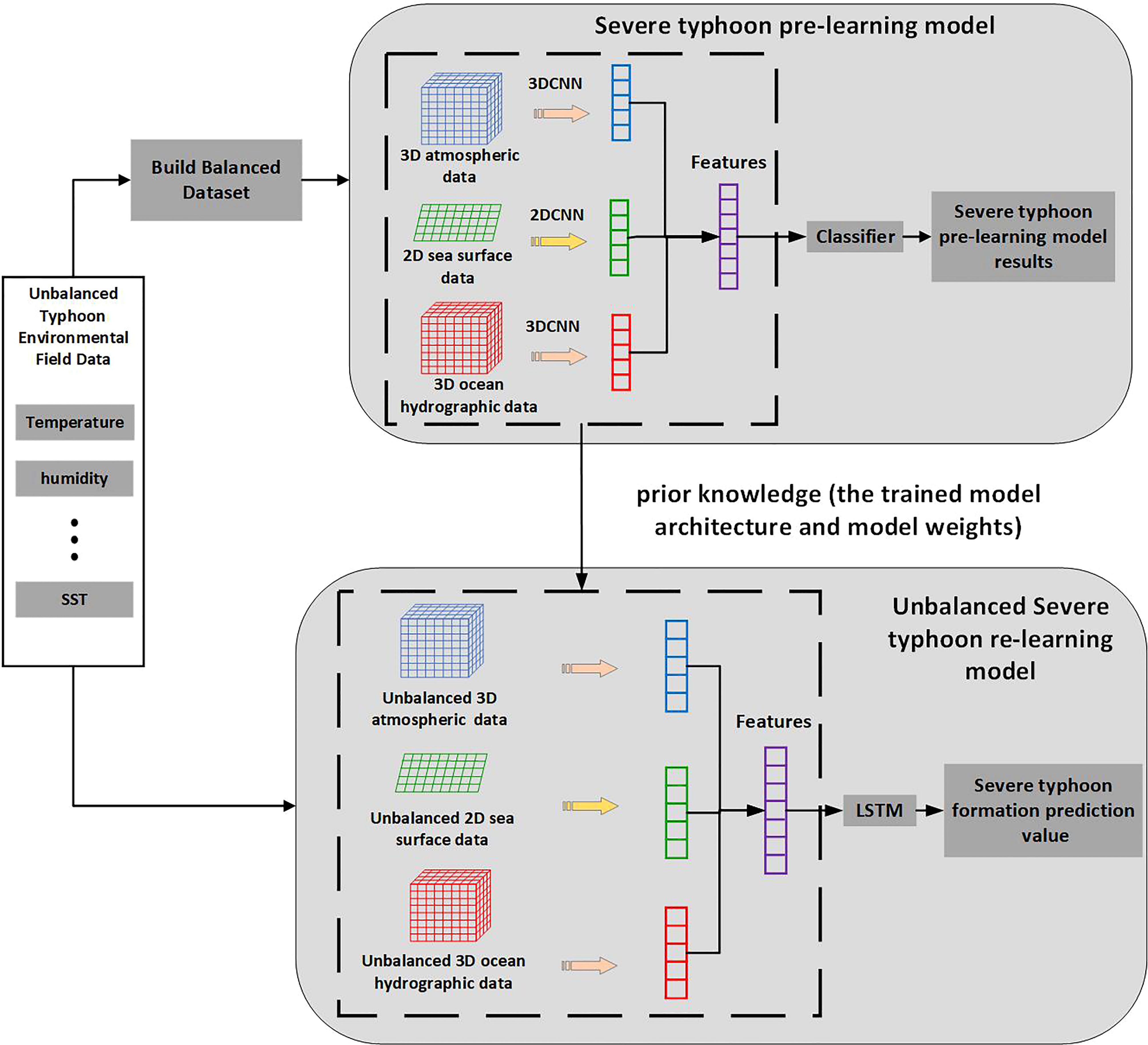
Figure 1 The overall structure of the USFP framework.

The first part is to learn from the balanced dataset. The structure and parameters of the feature extraction part learned from the balanced dataset are what we call prior knowledge in this paper. The severe typhoon pre-learning model uses 2D Convolutional Neural Networks (2DCNN) and 3D Convolutional Neural Networks (3DCNN) to extract features from high-dimensional data. The model weights are adjusted by adding classifiers. We train the severe typhoon pre-learning model by constructing a balanced dataset. The trained model architecture and the model weight parameters of the feature extraction part are saved as prior knowledge for transfer learning.

The second part is to apply the prior knowledge to train the unbalanced dataset. First, we transfer the obtained prior knowledge to the unbalanced severe typhoon re-learning model. Then, the unbalanced severe typhoon re-learning model with prior knowledge is trained using an unbalanced dataset. In addition, we design the unbalanced severe typhoon (UST) loss function to optimize the model by assigning different weights to the ordinary typhoon and the severe typhoon samples. Finally, the most accurate classification results are obtained by adjusting the parameters of the model and used as the USFP framework results of severe typhoon formation prediction.

4.2 Severe typhoon pre-learning model

To obtain prior knowledge, we construct a balanced dataset for training the severe typhoon pre-learning model according to the definition of positive and negative samples in Section 3. We fuse atmospheric variables, sea surface variables, and ocean hydrographic variables as prediction variables to form the typhoon environmental field data. We take temperature (t), relative humidity (rh), geopotential height (z), u-component of wind (u) and v-component of wind (v) as the basic atmospheric variables associated with typhoons. The sea surface temperature (sst) is used as the basic sea surface variable associated with typhoons. The seawater temperature (st), eastward seawater velocity (water_u) and northward seawater velocity (water_v) are used as the basic ocean hydrographic variables associated with typhoons. We classify and label these environmental variable datasets according to the typhoon historical best track dataset. The labeled data are sampled to construct a balanced dataset for training a severe typhoon pre-learning model.

We use different networks to extract the features of different environmental variables. Sea surface variables, as 2D environmental field information, need to be extracted features with a 2DCNN network. Atmospheric variables and ocean hydrographic variables, as 3D environmental field information, need to be extracted features with the 3DCNN network. By using the 2D convolution kernel and the 3D convolution kernel respectively, the corresponding 2D feature map and 3D feature map are obtained. The feature maps are passed through the flatten layer and the fully connected layer to obtain the feature vectors. The model structure and model weights of this part are used as prior knowledge extracted from the balanced dataset. The model architecture that is used as prior knowledge is shown in Figure 2.

FIGURE 2

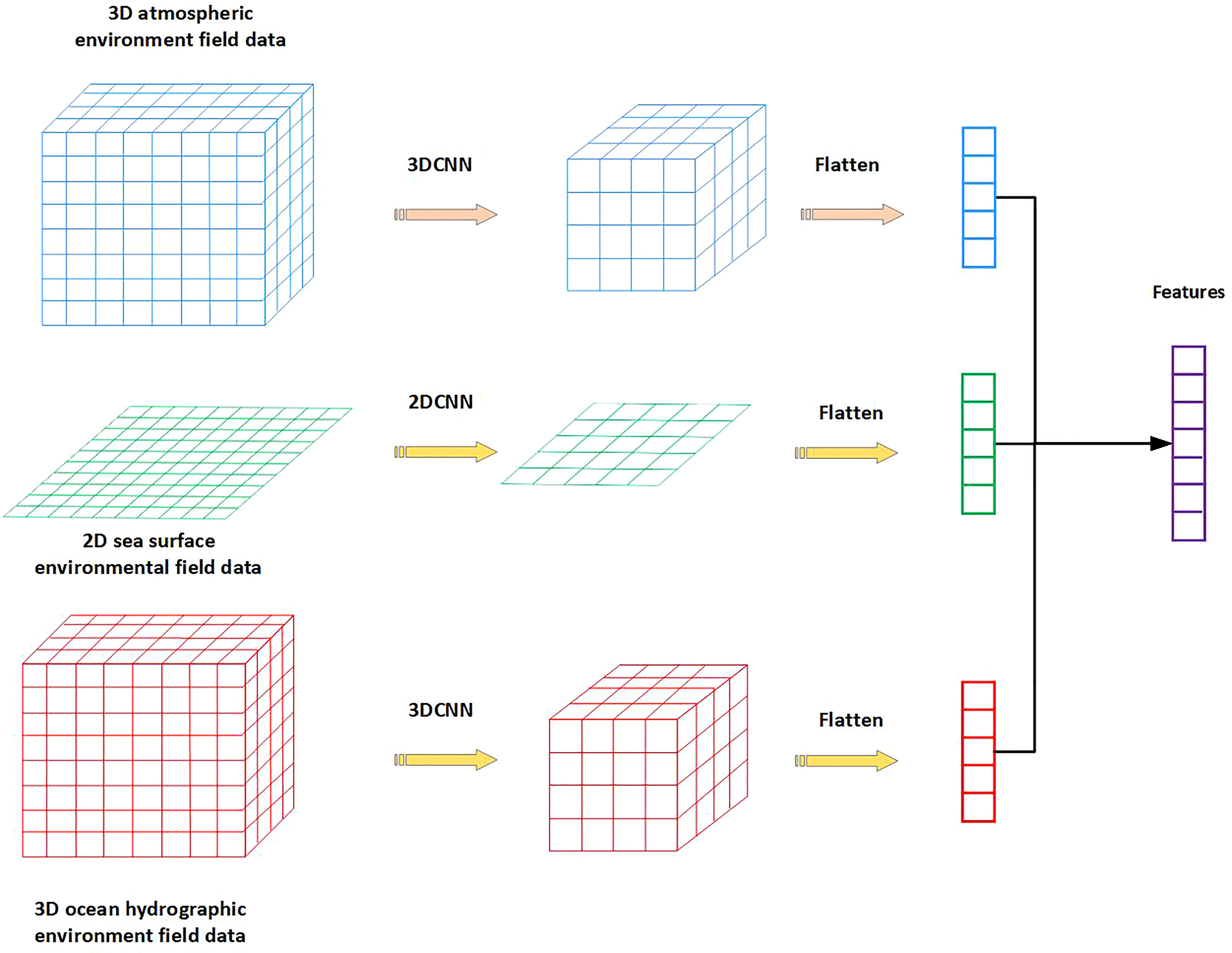
Figure 2 The model architecture used as prior knowledge in the strong typhoon pre-learning model.

According to the previous research (Chen et al., 2019), the structure of this feature extraction part is generalized into the formula as follows:

$\begin{array}{ll}\begin{array}{c}Features=Flatten\left(3DCNN\left(X_{t-6b}^P\right)\right)+Flatten\left(2DCNN\left(X_{t-6b}^S\right)\right)+\\ Flatten\left(3DCNN\left(X_{t-6b}^O\right)\right)\end{array}& (2)\end{array}$

The features learned by 3DCNN and 2DCNN are trained with the classifier. For the severe typhoon pre-learning model, we choose the commonly used binary cross-entropy loss function. The formula is as follows:

$\begin{array}{ll}\begin{array}{c}\begin{array}{c}Loss=-Y_{t+6k}log{Y}_{t+6k}^{\text{'}}-\left(1-Y_{t+6k}\right)log\left(1-Y_{t+6k}^{\text{'}}\right)=\{\begin{array}{c}-log{Y}_{t+6k}^{\text{'}}, Y_{t+6k}=1\\ -log\left(1-Y_{t+6k}^{\text{'}}\right), Y_{t+6k}=0\end{array}\end{array}\#\end{array}& (3)\end{array}$

Where $Y_{t+6k}^{\text{'}}$ is the model prediction result and Y_t+6k is the real label value. Y_t+6k  = 1 for positive samples and Y_t+6k  = 0 for negative samples.

The model architecture and model weights of the trained feature extraction part are saved as prior knowledge extracted from the balanced dataset for the next transfer learning step.

4.3 Unbalanced severe typhoon re-learning model

The unbalanced severe typhoon re-learning model is composed of the transferred feature extraction component (prior knowledge) and the LSTM model. The input to the unbalanced strong typhoon relearning model is the unbalanced dataset. The unbalanced dataset is trained with prior knowledge to obtain feature vectors, which are used as the input to the LSTM. The LSTM implements the prediction of strong typhoon formation.

The LSTM model is an improvement of the recurrent neural network model, which can keep the error at a constant level and enhance the robustness. Figure 3 shows the operations performed by the LSTM unit at time t, where X_t refers to the input at the current time, C_t−6 refers to the cell state 6 hours before time t, h_t−6 refers to the hidden state 6 hours before time t, and C_t refers to the information that can be stored in the LSTM cell. Through the three control units of input gate, output gate and forget gate in LSTM, it is determined which of the input information will be forgotten and which will be retained. Finally, the cell state C_t and the hidden state h_t corresponding to time t are obtained. LSTM can be represented as:

$\begin{array}{ll}\begin{array}{c}{h}_t,C_t=LSTM\left(\left[h_{t-6},X_t\right],C_{t-6}\right)\end{array}& (4)\end{array}$

FIGURE 3

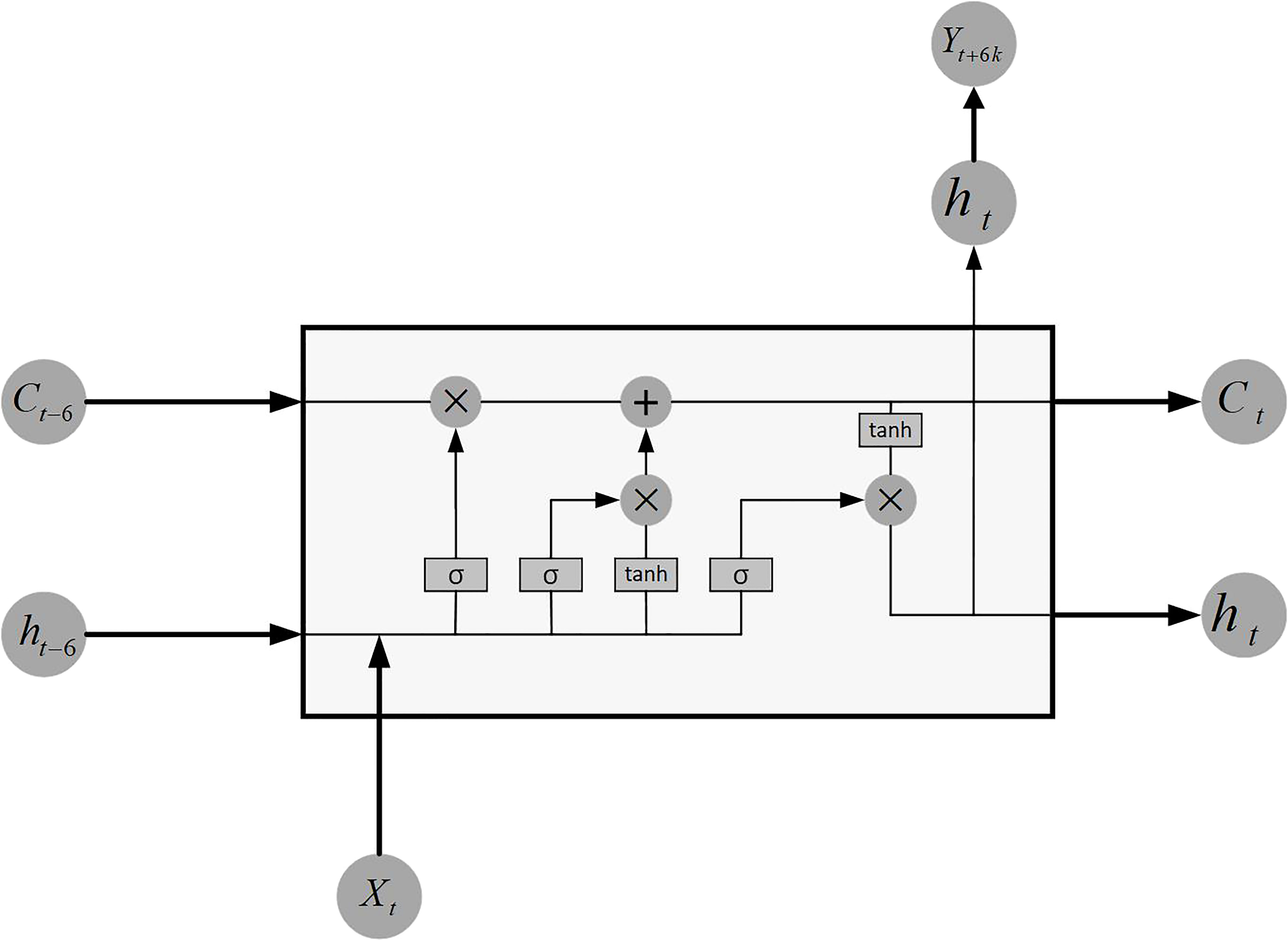
Figure 3 The classifier LSTM unit.

The LSTM model obtains the predicted value Y_t+6k after 6k hours at time t. Thereby, the unbalanced severe typhoon re-learning model can be expressed simply as:

$\begin{array}{ll}\begin{array}{c}{Y}_{t+6k}=LSTM\left(Features\left(X_{t-6b}^P,X_{t-6b}^S,X_{t-6b}^O\right)\right)\end{array}& (5)\end{array}$

We expect the unbalanced severe typhoon re-learning model to pay more attention to the severe typhoon samples in the classification process of unbalanced datasets. Therefore, the unbalanced severe typhoon loss function designed in this paper assigns different weights to the strong typhoon samples, which is calculated as follows:

$\begin{array}{ll}\begin{array}{c}UST Loss=\{\begin{array}{c}-\alpha {\left(1-Y_{t+6k}^{\text{'}}\right)}^{\gamma }log{Y}_{t+6k}^{\text{'}}, Y_{t+6k}=1\\ -\left(1-\alpha \right)Y_{t+6k}^{\text{'}\gamma }log\left(1-Y_{t+6k}^{\text{'}}\right), Y_{t+6k}=0\end{array}\#\end{array}& (6)\end{array}$

where γ is the weight factor used to focus on difficult and misclassified samples and α is the balance factor used to balance the unbalanced proportion of positive and negative samples. The higher the value of γ is set, the more it focuses on difficult samples. The value of α is appropriately weighted according to the sample ratio setting in the experiments. In the experiment, γ = 2 and α = 0.9. The analysis of γ is shown in Section 5.4.2.4.

After building the unbalanced strong typhoon relearning model, it is necessary to freeze and retrain the prior knowledge part of the model. Adjustments to the number of frozen and retrained layers are called fine-tuning operations in transfer learning. By freezing some layers in the prior knowledge, the number of training parameters of the model can be adjusted. In experiments, we try to find the best combination between the number of frozen layers and the number of retraining layers to achieve better predictions. The analysis of fine-tuning experimental results is presented in Section 5.4.2.1.

5 Experiments

This section details the experiments performed with the USFP framework. It mainly includes the experimental dataset, the evaluation metrics of the framework, the implementation of the experiment, and the analysis of the experiment results.

5.1 Datasets

The typhoon track dataset used in this paper is the World Meteorological Organization (WMO) version of the International Best Trajectory Archive for Climate Management (IBTrACS) Global Tropical Cyclone Best Trajectory Dataset. The atmospheric variable and sea surface variable dataset used in this paper are the ERA-Interim Reanalysis Dataset. The ocean hydrographic variable dataset used in this paper is the Hybrid Coordinate Ocean Model (HYCOM) dataset. The data for each moment of each typhoon in the three datasets correspond to each other. The first two datasets were recorded from 1979 to 2016. The ocean hydrographic datasets were recorded from 1994 to 2015. The wind speed is recorded every 6 hours from the time of tropical cyclone formation. Since typhoons are high-impact weather, the surrounding environmental fields change drastically. Therefore, high-resolution and multi-level data were selected during the experiment. According to previous research on high-dimensional data (Wang et al., 2021), this paper uses a neural network to reduce the dimension of high-dimensional data. In addition, compared with traditional deep learning datasets, typhoon forecasts need to ensure timeliness. The longer the timeliness of the general typhoon forecast business forecast, the more valuable it is for reference. But too long timeliness will also lead to a reduction in the number of training samples. Therefore, the prediction time of 24 hours was chosen to ensure a balance between the sample size and the timeliness of the model.

In the experiment, this paper selects typhoons in the Western Pacific (WP), Eastern Pacific (EP), and North Atlantic (NA) regions as samples. According to previous research (Camargo et al., 2007; Chen et al., 2019), temperature (t), relative humidity (rh), geopotential height (z), u component of wind (u), and v component of wind (v) are selected as atmospheric variables. The atmospheric pressure level of 1000/975/925/850/800/700/600/500/400/300/200/100hpa is chosen. Sea surface temperature (sst) is selected as the sea surface variable. According to previous research (Shay et al., 2000; Wu et al., 2007; Goni et al., 2009; Lin et al., 2009; Vissa et al., 2013), ocean heat content (UOHC), eddy currents and other ocean features play an important role in the intensification of tropical cyclones. Therefore, seawater temperature (st), eastward sea water velocity (water_u), and northward water velocity (water_v) are selected as ocean hydrographic variables. The ocean depth of 100/90/80/70/60/50/45/40/35/30/25/20/15/12/10/8/6/4/2m is chosen.

This part is about constructing input datasets and output datasets. For the 3DCNN part, the dimension of the input dataset is N×T×L×W×H×A or N×T×L×W×D×R. For the 2DCNN part, the dimension of the input dataset is N×T×L×W×O. For the LSTM classifier part, the dimension of the input dataset is N×T×K. Among them, N represents the number of samples. L and W range in 33 ~ 161. T represents the time step and T = 5. H = 12. D = 19. A = 5. R = 3. O = 1. K represents the length of the eigenvector. The samples at the moment when the maximum wind speed near the typhoon center value reaches the severe typhoon standard are marked as 1 and the rest of ordinary typhoons samples are marked as 0. In the experiment without ocean hydrographic variables, the data set is constructed by random sampling of the atmospheric environmental field data and the sea surface environmental field data. In the ocean hydrographic variables experiment, we intercept atmospheric and sea surface variables recorded from 1994 to 2015, which are recorded at the same time as the ocean hydrographic variables. After screening the original dataset, we constructed a balanced dataset with the same number of positive and negative samples and an unbalanced dataset with a positive and negative sample ratio of about 1:9 in different regions. The specific sample size is shown in Table 2. Furthermore, the dataset is split into a 70% training set and a 30% test set.

TABLE 2

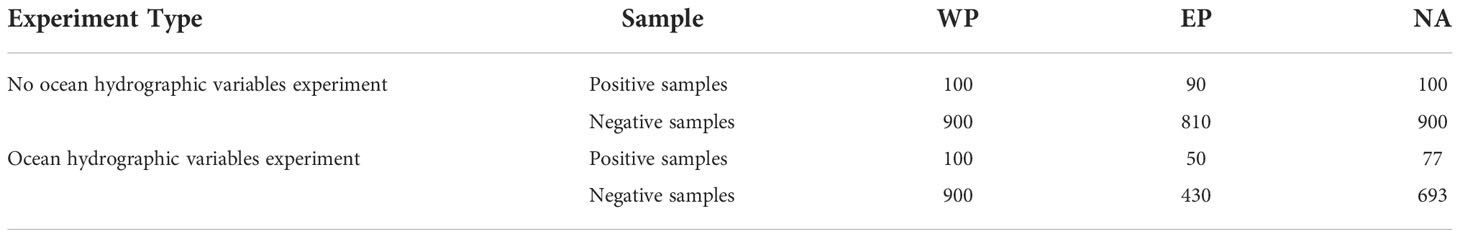
Table 2 The number of positive and negative samples in the experiment.

5.2 Evaluation metrics

To measure the performance of the model, the evaluation metric for traditional binary classification models is generally accuracy (Acc). The specific formula is as follows:

$\begin{array}{ll}\begin{array}{c}Acc=\frac{TP+TN}{TP+FN+FP+TN}\end{array}& (7)\end{array}$

However, it can be seen from the formula that when the dataset is unbalanced, the model training process will be more biased towards negative samples to make TN much larger than TP to obtain a larger Acc value. Therefore, according to the evaluation metrics selected when solving unbalanced data in the official Tensorflow document (Abadi et al., 2015), we select the values of ROC_AUC, PR_AUC, and F1 as evaluation metrics to measure the actual performance of the model.

ROC_AUC refers to the area under the ROC curve. The abscissa of the ROC curve is the false positive rate ($FPR=\frac{FP}{FP+TN}$) and the ordinate is the true positive rate ($TPR=\frac{TP}{TP+FN}$). The larger the ROC_AUC value, the more likely the current classification model will place positive samples in front of negative samples, which can better classify these samples.

$\begin{array}{ll}\begin{array}{c}ROC\_AUC={\int }^{}ROC\end{array}& (8)\end{array}$

PR_AUC refers to the area under the PR curve. The abscissa of the PR curve is the recall rate ($r\text{e}call=\frac{TP}{TP+FN}$) and the ordinate is the precision rate ($pr\text{e}c\text{i}s\text{i}on=\frac{TP}{TP+FP}$). When the PR_AUC value is larger, the positive sample classification effect is better.

$\begin{array}{ll}\begin{array}{c}PR\_AUC={\int }^{}PR\end{array}& (9)\end{array}$

F1 is the harmonic mean of precision and recall. Since the precision rate and the recall rate are contradictory to a certain extent, the F1 value is used to evaluate the precision rate and the recall rate as a whole.

$\begin{array}{ll}\begin{array}{c}F1=\frac{2\times pr\text{e}c\text{i}s\text{i}on\times r\text{e}call}{pr\text{e}c\text{i}s\text{i}on+r\text{e}call}\end{array}& (10)\end{array}$

5.3 Implementation

The USFP framework is implemented in tensorflow2.4 using Keras. The experimental model was trained using a Tesla V100 GPU card. Since there are some missing data in the typhoon environmental field dataset, the missing data are filled in and the whole data are normalized before the experiment. The constructed balanced dataset is used to train the severe typhoon pre-learning model.

In the severe typhoon pre-learning model 3DCNN module, three 3D convolutional layers, a maximum pooling layer, a flat layer, and a fully connected layer are used. For learning the atmospheric environmental field data features, the size of each layer of the convolutional layer is 5×5×1, the stride is 2×2×1, and the number of filters is 64, 64, and 128. The size of the max pooling layer is 5×5×1 and the stride is 2×2×1. For learning the characteristics of the ocean hydrographic environmental field data, the size of each layer of the convolutional layer is 3×3×1, the stride is 2×2×1, and the number of filters is 64, 64, and 128. The size of the max pooling layer is 3×3×1 and the stride is 2×2×1. The high-dimensional data is dimensionally reduced using a flatten layer. Both variables output 100 feature vectors through the fully connected layer. In the severe typhoon pre-learning model 2DCNN module, three 2D convolutional layers, one max pooling layer, one flatten layer, and one fully connected layer are used. The size of each layer of the convolutional layer is 5×5, the stride is 2×2, and the number of filters is 32, 64, and 128. The size of the max pooling layer is 5×5 and the stride is 2×2. The high-dimensional data is dimensionally reduced using a flatten layer. Then, the data outputs 100 feature vectors through the fully connected layer. Besides, the feature extraction part of this model needs to be encapsulated using the TimeDistributed layer wrapper to assign the same weights to the data in the time latitude. The activation function of all layers is ‘relu’.

After training the severe typhoon pre-learning model, the obtained prior knowledge is transferred to the unbalanced severe typhoon re-learning model and combined with LSTM for training. The L2 regularization is added to the fully connected layer to prevent overfitting of the model during training. After the framework structure is constructed, the hyperparameters are tuned to obtain the best prediction results.

5.4 Analysis

5.4.1 Result analysis

In order to prove that the USFP framework proposed in this paper can effectively improve the unbalanced data problem, experiments compare the framework with traditional machine learning-based methods. Since the environmental data used in this paper has a spatiotemporal dimension, in order to ensure the consistency of the comparative experiments, the machine learning model involved in the comparison needs to be able to consider the spatiotemporal relationship in the dataset. Therefore, this paper selects the ConvLSTM model (Shi et al., 2015), which can learn spatiotemporal features of data and the hybrid CNN_LSTM model (Chen et al., 2019), which has a good effect on typhoon formation and intensity prediction, as the comparison objects. As a spatiotemporal sequence prediction model, the ConvLSTM model can well capture the spatial information of the data based on the LSTM model. The typhoon spatiotemporal depth mixed prediction model [75] has a good performance in the formation of typhoon and the prediction of typhoon intensity, and the model has a high generalization ability. In addition, this paper also compares the proposed framework with other methods combining CNN and LSTM, such as 2DCNN+LSTM, 3DCNN+LSTM. Furthermore, since these models do not take into account the imbalance of data set samples, some traditional methods of dealing with imbalanced data are added to the original model for comparison. These machine learning model methods selected in the experiments all use the best parameters provided by the original author’s paper, and use the same training and test sets for training and testing. The specific experimental results are shown in Table 3.

TABLE 3

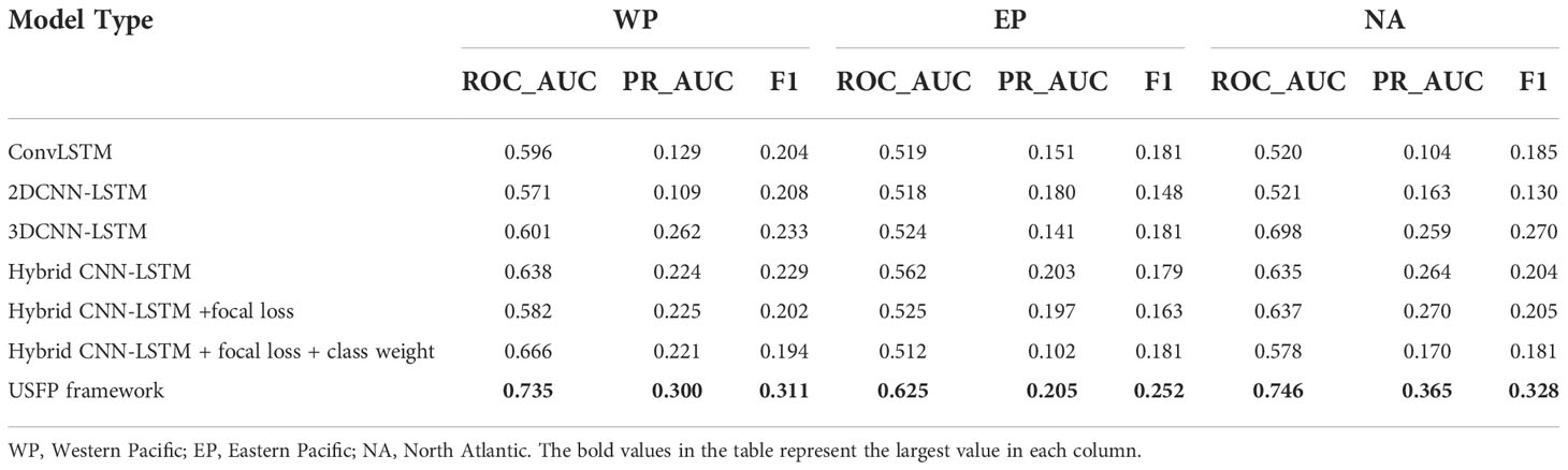
Table 3 Comparison of experimental results of different models.

As shown in Table 3, the USFP framework in the WP region can achieve the best ROC_AUC value of 0.735, the best PR_AUC value of 0.3, and the best F1 value of 0.311. In comparison, the best ROC_AUC of traditional machine learning-based methods is only 0.666, the best PR_AUC is only 0.262, and the best F1 is only 0.233. This is because traditional machine learning-based methods do not consider the unbalance of the data and the model cannot obtain good results based on the actual unbalanced dataset. In addition, the traditional methods of handling unbalanced data assign different weights to different samples based on the ratio between samples, which cannot reflect the actual distribution of data features. Therefore, these methods also cannot lead to better classification performance of the model. To ensure the generalization ability of the framework on different datasets and the robustness of the framework, experiments are also conducted on the EP and NA regions. In the EP region, the best ROC_AUC of traditional machine learning-based methods is 0.562, the best PR_AUC is 0.203, and the best F1 is 0.200. The USFP framework can achieve the best ROC_AUC value of 0.625, the best PR_AUC value of 0.205, and the best F1 value of 0.252. In the NA region, the best ROC_AUC of traditional machine learning-based methods is 0.698, the best PR_AUC is 0.270, and the best F1 is 0.270. The USFP framework can achieve the best ROC_AUC value of 0.746, the best PR_AUC value of 0.365, and the best F1 value of 0.328.

5.4.2 Parametric analysis

5.4.2.1 Fine tuning

The USFP framework is fine-tuned in the experiments according to the fine-tuning method in Section 4.3. The experimental results are shown in Figure 4. As the number of frozen layers increases, the three types of evaluation metrics fluctuate to varying degrees in different regions. Through experimental verification, it can be concluded that in the WP area, when there is no frozen layer, the PR_AUC value reaches the best value; and when the number of frozen layers is two, the F1 and ROC_AUC values reach the best value. In the NA area, when the number of frozen layers is 15, the three types of evaluation metrics all reach the best values. In the EP area, when the number of frozen layers is 8, the ROC_AUC value reaches the optimal value; when the number of frozen layers is 2, the F1 value and PR_AUC value reach the optimal value.

FIGURE 4

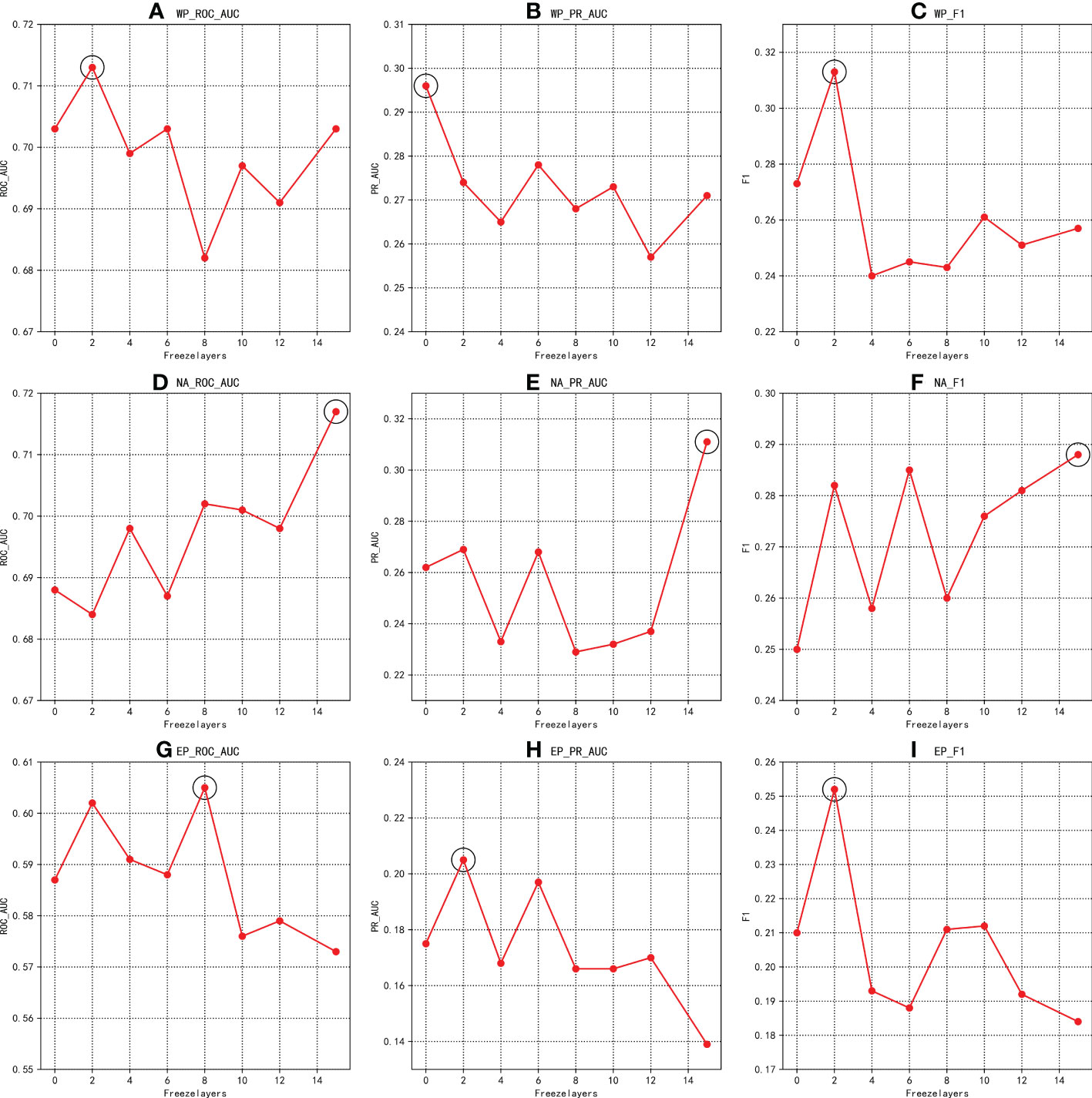
Figure 4 In different regions, the three types of evaluation metrics change with the number of frozen layers. (A–C) represent the results of the three indicators for the WP region. (D–F) represent the results of the three indicators for the NA region. (G–I) represent the results of the three indicators for the EP region.

5.4.2.2 Severe typhoon pre-learning model LR

The gradient descent algorithm is a commonly used optimization algorithm for deep learning, which can calculate the gradient through partial derivatives. The learning rate (LR) is one of the important parameters to control the update rate of parameters. According to previous studies (Kornblith et al., 2019), the learning effect of the severe typhoon pre-learning model has a great influence on the effect of the USFP framework. Therefore, the LR of the severe typhoon pre-learning model is selected as the adjustment parameter for analysis. The specific results are shown in Figure 5.

FIGURE 5

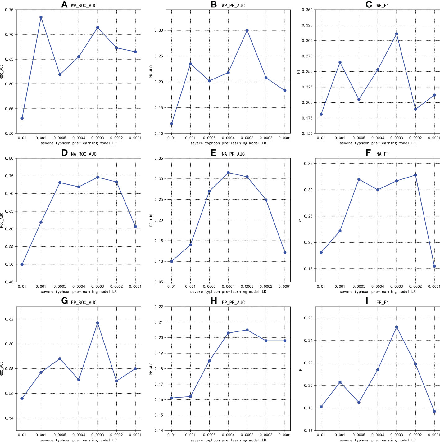
Figure 5 In different regions, the three types of evaluation metrics change with the severe typhoon pre-learning model LR. (A–C) represent the results of the three indicators for the WP region. (D–F) represent the results of the three indicators for the NA region. (G–I) represent the results of the three indicators for the EP region.

As shown in Figure 5, as the LR of the severe typhoon pre-learning model decreases, different metrics in different regions have certain fluctuations. In the WP region, ROC_AUC, PR_AUC, and F1 reach their maximum values when the severe typhoon pre-learning model LR is 0.001, 0.0003, and 0.0003 respectively. In the NA area, each metric increases and then decreases as the LR of the severe typhoon pre-learning model decreases. ROC_AUC, PR_AUC, and F1 reached the maximum value when the LR of the severe typhoon pre-learning model is 0.0003, 0.0004, and 0.0002 respectively. In the EP region, ROC_AUC, PR_AUC, and F1 all reach the maximum value when the severe typhoon pre-learning model LR is 0.0003. It can be concluded that when the LR value of the severe typhoon pre-learning model is selected as 0.0003, the unbalanced strong typhoon formation prediction framework has a good prediction effect in each region. Therefore, the LR value of the severe typhoon pre-learning model should be chosen to be 0.0003, so that the framework has better generalization ability.

5.4.2.3 Epochs

In this paper, we analyzed the epochs parameter to determine the period to obtain the best performance of the model. As shown in Figure 6, in both the WP region and the NA region, the ROC_AUC values tend to stabilize after 30 epochs of training. The ROC_AUC value in the EP region fluctuates relatively wildly, but after 10 rounds of training, the value is relatively stable within a certain range. Therefore, in our experiments, a relatively suitable training period is around 30 epochs.

FIGURE 6

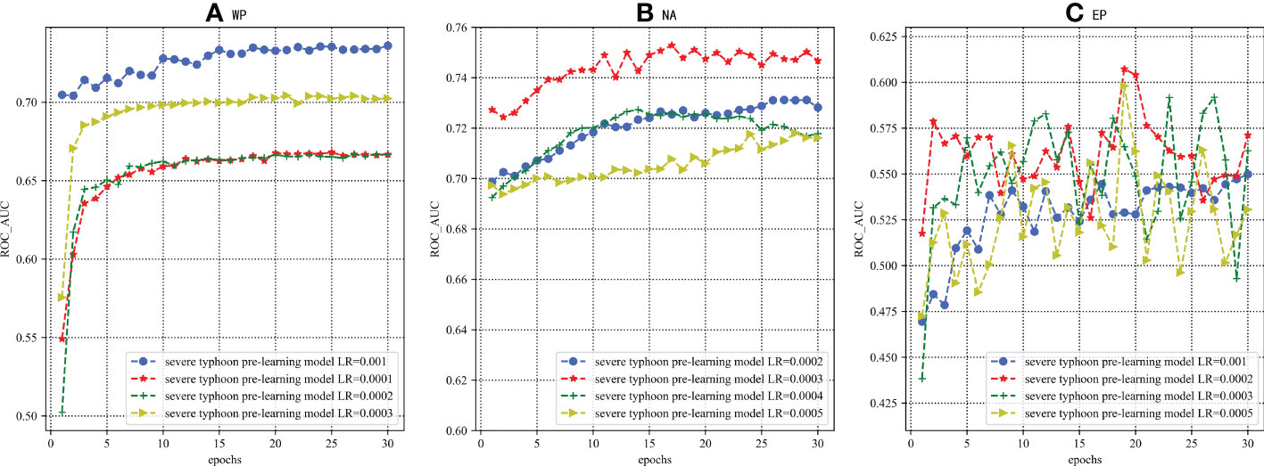
Figure 6 The ROC_AUC results with the change of epochs.

5.4.2.4 Weight factor

This section conducts a parametric analysis for the unbalanced severe typhoon loss function in the unbalanced severe typhoon re-learning model. Since the value of the balance factor α is determined by the sampling ratio in the experiment, the α is set to 0.9 in the experiments. We performed a parametric analysis of the weighting factor γ. As can be seen from the Table 4, the ROC_AUC value in the WP region increases and then decreases as γ increases. There are some fluctuations in the F1 and PR_AUC values in the WP region. When the γ is 2, the best effect of the model is achieved on the WP region. Therefore, the γ is set to 2 in this paper.

TABLE 4

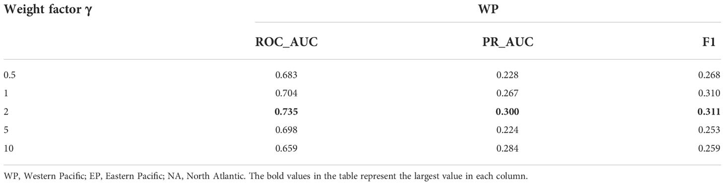
Table 4 Parametric analysis for weight factor γ.

5.4.3 Variables analysis

To study the influence of ocean hydrographic variables on the formation of severe typhoons, we selected seawater temperature (st), eastward seawater velocity (water_u), and northward current velocity (water_v) as ocean hydrographic variables. Atmospheric environmental field data, sea surface environmental field data, and ocean hydrographic environmental field data are used together as input data for the experiments. The experimental results are shown in Table 5.

TABLE 5

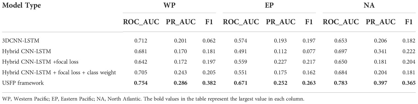
Table 5 Comparison of experimental results of different models after adding ocean hydrographic variables.

In the WP region, the USFP framework can achieve the best ROC_AUC value of 0.754, the best PR_AUC value of 0.286, and the best F1 value of 0.382. In comparison, the best ROC_AUC of traditional machine learning-based methods is only 0.712, the best PR_AUC is only 0.243, and the best F1 is only 0.205. In the EP region, the best ROC_AUC of the traditional machine learning-based method is 0.574, the best PR_AUC is 0.227, and the best F1 is 0.217. The USFP framework can achieve the best ROC_AUC value of 0.671, the best PR_AUC value of 0.252, and the best F1 value of 0.263. In the NA region, the best ROC_AUC of the traditional machine learning-based methods is 0.697, the best PR_AUC is 0.341, and the best F1 is 0.222. The USFP framework can achieve the best ROC_AUC value of 0.783, the best PR_AUC value of 0.397, and the best F1 value of 0.365.

Besides, we compare the experimental results with the ocean hydrographic variables to the experimental results without the ocean hydrographic variables. The comparison results are shown in Table 6. After adding the ocean hydrographic data, the evaluation metrics for all three regions (except the PR_AUC metric in the WP region) have improved. This proves that ocean hydrographic information has some influence on the formation of severe typhoons and helps to improve the accuracy of severe typhoon formation prediction.

TABLE 6

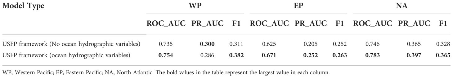
Table 6 Comparison of results between the USFP frameworks containing different environmental field variables.

5.4.4 Compare with the numerical model IFS

The numerical model prediction results used in this paper were obtained from the THORPEX Interactive Grand Global Ensemble (TIGGE) Model Tropical Cyclone Track Dataset. The dataset contains historical forecasting results for multiple official organizational models. We chose the historical forecasts of the European Centre for Medium-Range Weather Forecasts (ECMWF) ensemble forecast system (IFS), which has the longest record year in this dataset, as the object of comparison for the experiment. The historical forecast results document the predictions of tropical cyclone tracks from 2006 to 2016. Firstly, the temporal and central latitudinal and longitudinal positions provided by the World Meteorological Organization (WMO) version of the International Best Track Archive for Climate Management (IBTrACS) global tropical cyclone best track dataset are matched one-to-one with the historical prediction results of the IFS model to obtain the tropical cyclone samples. Secondly, the intensity values of tropical cyclone samples filtered from the global tropical cyclone best track dataset were used as labels to count the number of positive and negative samples for the three regions. The results are shown in Table 7.

TABLE 7

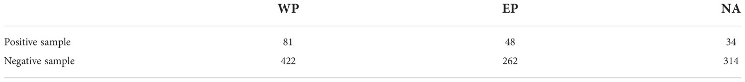
Table 7 The number of positive and negative samples screened by official data statistics.

Finally, the 24-hour step forecasts of the tropical cyclone samples filtered from the historical forecast results of the IFS model were used as model results and evaluated using the same evaluation metrics. The evaluation results are compared with the experimental results of the USFP framework. The comparison results are shown in Table 8.

TABLE 8

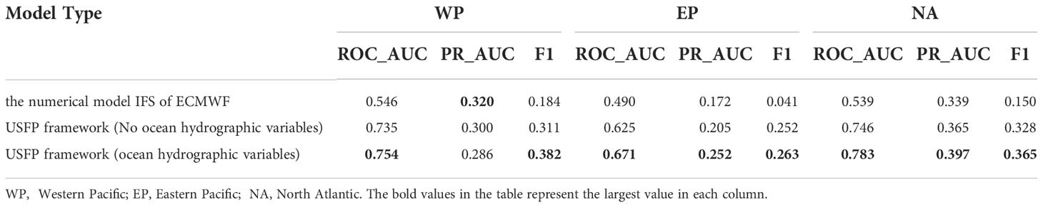
Table 8 Comparison of results between the USFP framework and the numerical model IFS of ECMWF.

The results of the USFP framework without ocean hydrographic variables and the USFP framework with ocean hydrographic variables outperform the prediction results of the IFS model for all metrics except the PR_AUC metric in the WP region. This proves that the USFP framework outperforms the numerical model IFS of ECMWF in the field of unbalanced severe typhoon formation prediction.

5.4.5 Example prediction

We performed a USFP framework forecast using the example of strong typhoon Roke in 2011. The generation of strong typhoon was successfully predicted by using USFP framework. The value of F1 is 1 because there is only one positive sample for a single sample and the calculated value of ROC_AUC is 0.734 and the calculated value of PR_AUC is 0.2. By checking the historical prediction results of the numerical model IFS of ECMWF, we can conclude that the numerical model did not accurately predict the generation of severe typhoons.

6 Conclusions and future work

In this paper, we define the severe typhoon formation prediction problem as a classification problem of spatio-temporal series prediction and propose an unbalanced severe typhoon formation prediction (USFP) framework. The framework fuses atmospheric, sea surface, and ocean hydrographic variables and uses a severe typhoon pre-learning model to obtain prior knowledge from the constructed balanced dataset. Then, we transfer the prior knowledge to the severe typhoon re-learning model to predict the formation of severe typhoons. Extensive experiments show that the USFP framework proposed in this paper is more accurate than the numerical model IFS of ECMWF and existing machine learning models.

Additional analysis and experiments on the parameters of the framework can lead to better results of the framework. We analyzed three parameters in our experiments: the number of frozen layers, the LR of the severe typhoon pre-learning model, and the number of epochs. The number of freezing layers is 2 or 15 layers to obtain better results. The optimal LR of the severe typhoon pre-learning model is 0.0003. The optimal epochs to adjust the iterations is about 30 rounds. In addition, we conducted a comparative experiment on the choice of environmental field variables. The experimental results show that adding the ocean hydrographic environmental field variables can help improve the prediction effect of the framework on the formation of severe typhoons.

In the future, we will further refine the details of the parameters in the USFP framework and use various data such as satellite image data to improve the framework functionality. In addition, since the framework is purely data-driven, it suffers from the problem of uninterpretability. Therefore, in further developmental work, we will try to integrate this framework with traditional physical models to improve the application ability of the model in practical systems.

Data availability statement

Publicly available datasets were analyzed in this study. This data can be found here: https://www.ncdc.noaa.gov/ibtracs/, https://www.ecmwf.int/en/forecasts/datasets/reanalysis-datasets/era-interim, https://www.hycom.org/dataserver/gofs-3pt1/reanalysis, https://rda.ucar.edu/datasets/ds330.3/index.html#!description.

Author contributions

XP and XW developed the idea. XP designed the research, analyzed the data, and wrote the manuscript. XW guided the whole study and revised the manuscript. CZ provides support and assistance on dataset acquisition. XW, HW, and SW helped to revise the manuscript. XW, HW, SW, and JW gave comments on the manuscript. SC helped with the English translation of the manuscript. All authors contributed to the article and approved the submitted version.

Funding

This research is partially supported by the National Natural Science Foundation of China (42276205) and the National Natural Science Foundation of China (41875121).

Acknowledgments

Special thanks to the Institute of Numerical Meteorology and Oceanography, College of Meteorology and Oceanography, National University of Defense Technology for the equipment support.

Conflict of interest

The authors declare that the research was conducted in the absence of any commercial or financial relationships that could be construed as a potential conflict of interest.

Publisher’s note

All claims expressed in this article are solely those of the authors and do not necessarily represent those of their affiliated organizations, or those of the publisher, the editors and the reviewers. Any product that may be evaluated in this article, or claim that may be made by its manufacturer, is not guaranteed or endorsed by the publisher.

References

Abadi M., Barham P., Chen J., Chen Z., Davis A., Dean J., et al. (2015). TensorFlow: Large-scale machine learning on heterogeneous systems. In 12th USENIX symposium on operating systems design and implementation. (OSDI 16) (pp. 265–283).

Google Scholar

Ahijevych D., Pinto J. O., Williams J. K., Steiner M. (2016). Probabilistic forecasts of mesoscale convective system initiation using the random forest data mining technique. (Boston MA, USA: Weather & Forecasting) 31 (2), 581–599.

Google Scholar

Al-Stouhi S., Reddy C. K. (2016). Transfer learning for class imbalance problems with inadequate data. Knowledge Inf. Syst. 48 (1), 201–228. doi: 10.1007/s10115-015-0870-3

CrossRef Full Text | Google Scholar

Camargo S. J., Emanuel K. A., Sobel A. H. (2007). Use of a genesis potential index to diagnose enso effects on tropical cyclone genesis. J. Climate 20 (19), 4819–4834. doi: 10.1175/JCLI4282.1

CrossRef Full Text | Google Scholar

Chen R., Wang X., Zhang W., Zhu X., Li A., Yang C. (2019). A hybrid CNN-LSTM model for typhoon formation forecasting. GeoInformatica 23 (3), 375–396. doi: 10.1007/s10707-019-00355-0

CrossRef Full Text | Google Scholar

China Meteorological Administration (2020). China Meteorological disaster yearbook 2019 (Beijing, China: Meteorological Press).

Google Scholar

Combinido J. S., Mendoza J. R., Aborot J. (2018). “A convolutional neural network approach for estimating tropical cyclone intensity using satellite-based infrared images,” in International Conference on Pattern Recognition. (Chinese Acad Sci, Inst Automat, Beijing, PEOPLES R CHINA: IEEE), 1474–1480.

Google Scholar

Cui Y., Jia M., Lin T. Y., Song Y., Belongie S. (2019). “Class-balanced loss based on effective number of samples,” in IEEE Conference on Computer Vision and Pattern Recognition. (Long Beach, CA: IEEE Comp Soc).

Google Scholar

Demaria M., Kaplan J. (1994). A statistical hurricane intensity prediction scheme (ships) for the atlantic basin. Wea Forecasting 9 (2), 209–220. doi: 10.1175/1520-0434(1994)009<0209:ASHIPS>2.0.CO;2

CrossRef Full Text | Google Scholar

DeMaria M., Kaplan J. (1999). An updated statistical hurricane intensity prediction scheme (SHIPS) for the Atlantic and Eastern north pacific basins Vol. 14 (Boston MA, USA: Weather & Forecasting), 326–337.

Google Scholar

Deo R. V., Chandra R., Sharma A. (2017). Stacked transfer learning for tropical cyclone intensity prediction. arXiv preprint arXiv:1708.06539. doi: 10.48550/arXiv.1708.06539

CrossRef Full Text | Google Scholar

Elsberry R. L., Tsai H. C., Chin W. C., Marchok T. P. (2021). Predicting rapid intensification events following tropical cyclone formation in the western north pacific based on ecmwf ensemble warm core evolutions. Atmosphere 12. doi: 10.3390/atmos12070847

PubMed Abstract | CrossRef Full Text | Google Scholar

Fei T., Huang B., Wang X., Zhu J., Chen Y., Wang H., et al. (2022). A hybrid deep learning model for the bias correction of SST numerical forecast products using satellite data. Remote Sens. 14 (6), 1339. doi: 10.3390/rs14061339

CrossRef Full Text | Google Scholar

Fritsch J. M., Chappell C. F. (1980). Numerical prediction of convectively driven mesoscale pressure systems. part II. mesoscale model. J. Atmospheric Sci. 37 (8), 1734–1762. doi: 10.1175/1520-0469(1980)037<1734:NPOCDM>2.0.CO;2

CrossRef Full Text | Google Scholar

Geng Y., Luo X. (2019). Cost-sensitive convolutional neural networks for imbalanced time series classification. Intelligent Data Analysis 23 (2), 357–370.

Google Scholar

Goni G., DeMaria M., Knaff J., Sampson C., Ginis I., Bringas F., et al. (2009). Applications of satellite-derived ocean measurements to tropical cyclone intensity forecasting. Oceanography 22 (3), 190–197. doi: 10.5670/oceanog.2009.78

CrossRef Full Text | Google Scholar

Halperin D. J., Fuelberg H. E., Hart R. E., Cossuth J. H., Sura P., Pasch R. J. (2013). An evaluation of tropical cyclone genesis forecasts from global numerical models. Weather Forecasting 28 (6), 1423–1445.

Google Scholar

Han H., Wang W. Y., Mao B. H. (2005). Borderline-smote: a new over-sampling method in imbalanced data sets learning (Beijing, China: Lecture Notes in Computer Science).

Google Scholar

Higa M., Tanahara S., Adachi Y., Ishiki N., Nakama S., Yamada H., et al. (2021). Domain knowledge integration into deep learning for typhoon intensity classification. Sci. Rep. 11 (1), 1–10. doi: 10.1038/s41598-021-92286-w

PubMed Abstract | CrossRef Full Text | Google Scholar

Hu Z., Li X., Tu C., Liu Z., Sun M.. (2018). “Few-shot charge prediction with discriminative legal attributes[C],” in Proceedings of the 27th International Conference on Computational Linguistics. (Santa Fe, New Mexico, USA: Association for Computational Linguistics), 487–498.

Google Scholar

John P. C. (2019). National hurricane center forecast verification report, (2019) (Miami, FL, USA: National Hurricane Center).

Google Scholar

Kim M., Park M. S., Im J., Park S., Lee M. I. (2019). Machine learning approaches for detecting tropical cyclone formation using satellite data. Remote Sens. 11 (10), 1195. doi: 10.3390/rs11101195

CrossRef Full Text | Google Scholar

Knaff J. A., Sampson C. R., Demaria M. (2005). An operational statistical typhoon intensity prediction scheme for the western north pacific Vol. 20 (Boston MA, USA: Weather & Forecasting), 688–699.

Google Scholar

Kornblith S., Shlens J., Le Q. V. (2019). “Do better imagenet models transfer better?,” in IEEE Conference on Computer Vision and Pattern Recognition. (Long Beach, CA: IEEE Comp Soc), 2661–2671.

Google Scholar

Lee H., Park M., Kim J. (2016). “Plankton classification on imbalanced large scale database via convolutional neural networks with transfer learning,” in IEEE International Conference on Image Processing ICIP. (Phoenix, AZ: IEEE), 3713–3717.

Google Scholar

Lin I. I., Chen C. H., Pun I. F., Liu W. T., Wu C. C. (2009). Warm ocean anomaly, air sea fluxes, and the rapid intensification of tropical cyclone nargis. Geophys Res. Lett. 36, L03817. doi: 10.1029/2008GL035815

CrossRef Full Text | Google Scholar

Lin T. Y., Goyal P., Girshick R., He K., Dollár P. (2017). Focal loss for dense object detection. IEEE Trans. Pattern Anal. Mach. Intell. 99, 2999–3007. doi: 10.1109/iccv.2017.324

CrossRef Full Text | Google Scholar

Liu X. Y., Wu J., Zhou Z. H. (2009). Exploratory undersampling for class-imbalance learning. IEEE Trans. Syst. Man Cybernetics Part B 39 (2), 539–550. doi: 10.1109/tsmcb.2008.2007853

CrossRef Full Text | Google Scholar

Long M., Cao Y., Wang J., Jordan M. (2015). “Learning transferable features with deep adaptation networks,” in International conference on machine learning ((Lille, FRANCE: PMLR), 97–105.

Google Scholar

Matsuoka D., Nakano M., Sugiyama D., Uchida S. (2018). Deep learning approach for detecting tropical cyclones and their precursors in the simulation by a cloud-resolving global nonhydrostatic atmospheric model Vol. 5 (Japan: Progress in Earth and Planetary Science).

Google Scholar

Mecikalski J. R., Sandmæl T. N., Murillo E. M., Homeyer C. R., Bedka K. M., Apke J. M., et al. (2021). A random-forest model to assess predictor importance and nowcast severe storms using high-resolution radar–GOES satellite–lightning observations. Monthly Weather Review 149 (6), 1725–1746. doi: 10.1175/MWR-D-19-0274.1

CrossRef Full Text | Google Scholar

Mo X., Jiao H., Liu Y., Zhang J. (2019). “A classification algorithm of unbalanced data samples based on ResNet. RCAE 2019,” in RCAE 2019: Proceedings of the 2019 The 2nd International Conference on Robotics, Control and Automation Engineering. (New York, NY, United States: Association for Computing Machinery).

Google Scholar

Na W., McBride J. L., Zhang X.-H., Duan Y. H.. (2018). Understanding biases in tropical cyclone intensity forecast error. (Boston MA, USA: Weather & Forecasting) 33 (1), 129–138.

Google Scholar

Pang S., Xie P., Xu D., Meng F., Tao X., Li B., et al. (2021). NDFTC: A new detection framework of tropical cyclones from meteorological satellite images with deep transfer learning. Remote Sens. 13 (9), 1860. doi: 10.3390/rs13091860

CrossRef Full Text | Google Scholar

Park M. S., Kim M., Lee M. I., Im J., Park S. (2016). Detection of tropical cyclone genesis via quantitative satellite ocean surface wind pattern and intensity analyses using decision trees. Remote Sens. Environ. 183, 205–214. doi: 10.1016/j.rse.2016.06.006

CrossRef Full Text | Google Scholar

Reichstein M., Camps-Valls G., Stevens B., Jung M., Denzler J., Carvalhais N., et al. (2019). Deep learning and process understanding for data-driven earth system science. Nature 566 (7743), 195. doi: 10.1038/s41586-019-0912-1

PubMed Abstract | CrossRef Full Text | Google Scholar

Richman M. B., Leslie L. M., Ramsay H. A., Klotzbach P. J. (2017). Reducing tropical cyclone prediction errors using machine learning approaches. Proc. Comput. Sci. 114, 314–323. doi: 10.1016/j.procs.2017.09.048

CrossRef Full Text | Google Scholar

Shay L. K., Goni G. J., Black P. G. (2000). Effects of a warm oceanic feature on hurricane opal. Mon Weather Rev. 128, 1366–1383. doi: 10.1175/1520-0493(2000)128<1366:EOAWOF>2.0.CO;2

CrossRef Full Text | Google Scholar

Shi X., Chen Z., Wang H., Yeung D. Y., Wong W. K., Woo W. C. (2015). Convolutional LSTM network: A machine learning approach for precipitation nowcasting Vol. 28 (Montreal, CANADA: Advances in neural information processing systems).

Google Scholar

Singh R., Ahmed T., Kumar A., Singh A. K., Pandey A. K., Singh S. K. (2020). Imbalanced breast cancer classification using transfer learning. IEEE/ACM Trans. Comput. Biol. Bioinf. 18 (1), 83–93. doi: 10.1109/TCBB.2020.2980831

CrossRef Full Text | Google Scholar

Taherkhani A., Cosma G., McGinnity T. M. (2020). AdaBoost-CNN: An adaptive boosting algorithm for convolutional neural networks to classify multi-class imbalanced datasets using transfer learning. Neurocomputing 404, 351–366. doi: 10.1016/j.neucom.2020.03.064

CrossRef Full Text | Google Scholar

Troncoso A., Ribera P., Asencio-Cortés G., Vega I., Gallego D. (2018). Imbalanced classification techniques for monsoon forecasting based on a new climatic time series. Environ. Model. software 106, 48–56. doi: 10.1016/j.envsoft.2017.11.024

CrossRef Full Text | Google Scholar

Vissa N. K., Satyanarayana A. N. V., Kumar B. P. (2013). Intensity of tropical cyclones during pre-and post-monsoon seasons in relation to accumulated tropical cyclone heat potential over bay of Bengal. Nat. Hazard 68 (2), 351–371. doi: 10.1007/s11069-013-0625-y

CrossRef Full Text | Google Scholar

Wang X., Li X., Zhu J., Xu Z., Ren K., Zhang W., et al. (2021). “A local similarity-preserving framework for nonlinear dimensionality reduction with neural networks,” in International conference on database systems for advanced applications (Cham: Springer), 376–391.

Google Scholar

Wijnands J. S., Qian G., Kuleshov Y. (2016). Variable selection for tropical cyclogenesis predictive modeling. Monthly Weather Rev. 144 (12), 4605–4619. doi: 10.1175/mwr-d-16-0166.1

CrossRef Full Text | Google Scholar

Wikner A., Pathak J., Hunt B. R., Szunyogh I., Girvan M., Ott E. (2021). Using data assimilation to train a hybrid forecast system that combines machine-learning and knowledge-based components. Chaos (Woodbury, N.Y.) 31 (5), 053114. doi: 10.1063/5.0048050

PubMed Abstract | CrossRef Full Text | Google Scholar

Wu C. C., Lee C. Y., Lin I. I. (2007). The effect of the ocean eddy on tropical cyclone intensity. J. Atmos Sci. 64 (10), 3562–3578. doi: 10.1175/JAS4051.1

CrossRef Full Text | Google Scholar

Yan Q., Cao Y. (2019). Optimizing shapelets quality measure for imbalanced time series classification Vol. 4) (Netherlands: Applied Intelligence).

Google Scholar

Yip Z. K., Yau M. K. (2011). Application of artificial neural networks on north atlantic tropical cyclogenesis potential index in climate change. J. Atmospheric Oceanic Technol. 29 (9), 1202–1220. doi: 10.1175/jtech-d-11-00178.1

CrossRef Full Text | Google Scholar

Yosinski J., Clune J., Bengio Y., Lipson H. (2014). How transferable are features in deep neural networks? (Montreal, CANADA: MIT Press).

Google Scholar

Zhan F. (2020). “Research on bank fraud transaction detection based on LSTM-focalloss,” in ACAI 2020: 2020 3rd International Conference on Algorithms, Computing and Artificial Intelligence. (New York, NY, United States: Association for Computing Machinery).

Google Scholar

Zhang W., Fu B., Peng M. S., Li T.. (2015). Discriminating developing versus nondeveloping tropical disturbances in the western north pacific through decision tree analysis (Boston MA, USA: Weather & Forecasting) 30 (2), 446–454.

Google Scholar

Zhang T., Lin W., Lin Y., Zhang M., Xue W. (2019). Prediction of tropical cyclone genesis from mesoscale convective systems using machine learning Vol. 34 (Boston MA, USA: Weather and Forecasting).

Google Scholar