Research on outlier detection in CTD conductivity data based on cubic spline fitting

Outlier detection is the key to the quality control of marine survey data. For the detection of outliers in Conductivity-Temperature-Depth (CTD) data, previous methods, such as the Wild Edit method and the Median Filter Combined with Maximum Deviation method, mostly set a threshold based on statistics. Values greater than the threshold are treated as outliers, but there is no clear specification for the selection of threshold, thus multiple attempts are required. The process is time-consuming and inefficient, and the results have high false negative and positive rates. In response to this problem, we proposed an outlier detection method in CTD conductivity data, based on a physical constraint, the continuity of seawater. The method constructs a cubic spline fitting function based on the independent points scheme and the cubic spline interpolation to fit the conductivity data. The maximum fitting residual points will be flagged as outliers. The fitting stops when the optimal number of iterations is reached, which is automatically obtained by the minimum value of the sequence of maximum fitting residuals. Verification of the accuracy and stability of the method by means of examples proves that it has a lower false negative rate (17.88%) and false positive rate (0.24%) than other methods. Indeed, rates for the Wild Edit method are 56.96% and 2.19%, while for the Median Filter Combined with Maximum Deviation method rates are 23.28% and 0.31%. The Cubic Spline Fitting method is simple to operate, the result is clear and definite, better solved the problem of conductivity outliers detection.

1 Introduction

Oceanographic observations are the basis for assessing the physical and biochemical environment in the ocean, and accurate and reliable observations are crucial (Zhang et al., 2017; Chen et al., 2019; Liu et al., 2020). Marine science (including climate change studies, physical oceanography studies, ocean model development, and monitoring and prediction of marine ecological disasters) strongly relies on high-quality observed data (Davis et al., 2019; Roemmich et al., 2019; Yu et al., 2020; Zou et al., 2020). The quality of observation data is affected by a variety of factors such as instrument errors, equipment failures, external disturbances, transcoding errors, communication errors and serious errors. In addition, observed data may come from different countries (institutions), cruises, instruments, formats, and collection methods. Bit data are highly heterogeneous (Balmaseda et al., 2013; Palmer et al., 2017; Boyer et al., 2018). Even though the observed data are collected by the same type of instrument, there are still differences between them in consideration of sensors, sampling resolution or calibration procedures (Xu and Su, 1999; Thomson and Emery, 2014; WU et al., 2019). Due to these factors, observational errors are prevalent in oceanographic observation data and are difficult to detect and eliminate. And if issues related to data quality are not properly addressed, oceanographic data cannot be utilized in data management and scientific applications properly (Tan et al., 2021). Therefore, it is crucial to detect bad data accurately and effectively through quality control to ensure the overall reliability of in situ observations (Chen et al., 2019; Liu et al., 2020).

The Conductivity-Temperature-Depth (CTD) sensor is the most basic instrument used in ocean observation (Bushnell, 2020), and the amount of CTD data is also the most abundant (Good et al., 2013). Previous researchers have done plenty of work on the quality control of CTD data (Boyer et al, 1994; Gouretski and Cheng, 2020; Gourrion et al., 2020; Wong et al., 2021; Brunton and Kutz, 2022). The key submodules of CTD data quality control that have been widely used in previous studies include range check, continuity check, statistical feature check, vertical gradient check et cetera, and the spikes check which is addressed in this paper (Tan et al., 2021). Points with gradients greater than a chosen threshold are usually labeled as ‘spikes’ (Sy, 1983; Xu and Su, 1999; Gouretski, 2018), and the choice of a threshold is generally determined by statistical methods. The quality control of Sea-Bird series CTD data is basically carried out in accordance with the processing steps of SBE (Sea-Bird Electronics) Data Processing-Win32 software. Through hysteresis correction and thermal effect correction, large data ‘spikes’ caused by asynchrony between various sensors can be eliminated (Lueck, 1990; Morison et al., 1994; Mensah et al., 2018). The statistical PauTa criterion method has been used to find small random errors, for instance, in normally distributed data, values beyond ​​the ±3σ range will be treated as bad data (Sea-Bird Electronics, 2013; Liu et al., 2016; Yang et al., 2017). However, statistical methods are not appropriate for all cases. If the CTD observation data do not approximately obey the Gaussian distribution, the PauTa criterion won’t be effective (Tan et al., 2021). Finally, the selection of the threshold needs constant trial according to the quality of the original data (Sea-Bird Electronics, 2013). So, the results have great uncertainty and often lead to a higher false positive and negative rate.

According to the continuity of seawater, the marine elements at the same location change continuously. Based on this physical constraint, a fitting function can help construct the marine elements, and the difference between the observed value and the fitted data larger than the given threshold will be discriminated as outliers (Tan et al., 2021). The cubic spline fitting function has become an extremely important numerical fitting method due to its good stability and smoothness, and it has achieved good application results in data analysis (Jiang et al., 2018; Jin et al., 2018; Zong et al., 2018; Wang et al., 2019; Xu et al., 2021). Based on the above situation, this paper aims to propose an outlier detection method based on Cubic Spline Fitting. We apply it to the analysis of 20 CTD conductivity profile data, and compare it with the two common outlier detection methods to verify the feasibility of the method.

This paper is organized as follows. The second part introduces the data used and describes the operation steps of the Wild Edit (WE) method, the Median Filter Combined with Maximum Deviation method (MFMD) and the Cubic Spline Fitting method (CSF). In the third part, we compare and analyze the processing results of the three methods, and conclusions are drawn in the fourth part.

2 Data and methods

2.1 Data description

The 20 CTD profiles used in this paper were observed in the East China Sea (25°N-32°N, 121°E-128°E) with the SBE 911plus CTD system. The observation system is equipped with two temperature and conductivity sensors at the same time, and the sampling frequency is 24Hz. The temperature sensor has a resolution of 0.0002°C and an accuracy of 0.001°C. The conductivity sensor has a resolution of 0.0004 mS/cm and an accuracy of 0.003 mS/cm. The pressure sensor has a resolution of 0.06895 dbar (0.001% FS(Full-Scale)) and an accuracy of 1.034 dbar (0.015%FS).

Each of the 20 CTD profiles has two temperature (Figures 1A, C) and conductivity (Figures 1B, D) profiles, relative to the sensor couples. It can be seen from Figure 1 that one set of conductivity data has obvious bad data (Figure 1B), while the other conductivity profiles and the temperature profile don’t have errors (Figures 1A, C, D).

FIGURE 1

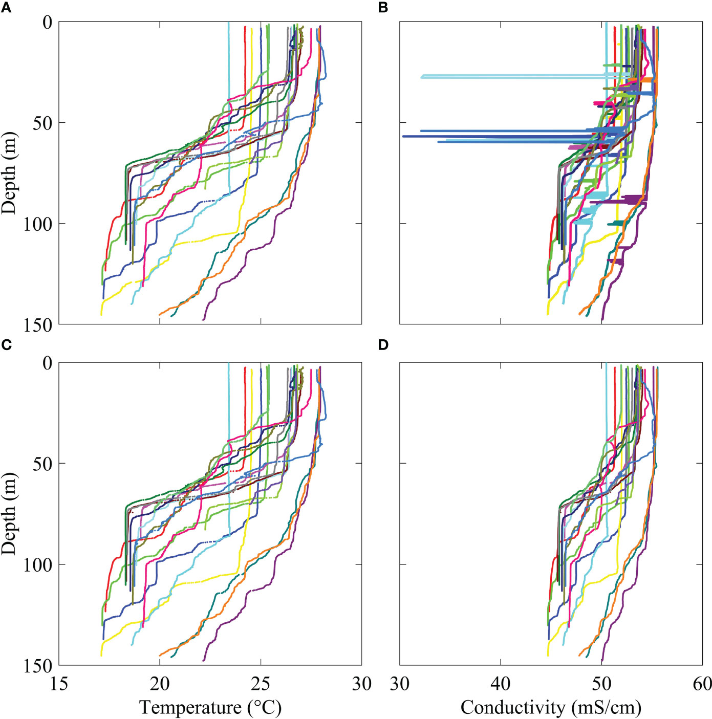
Figure 1 The 20 CTD conductivity and temperature profiles treated in this work. A, C and B, D represent two sets of temperature and conductivity data, respectively.

2.2 Methods

The common CTD outlier detection methods include the WE method used in the SBE Data Processing software (Sea-Bird Electronics, 2013), and the MFMD method proposed by Alexander Sy (Sy, 1983). This section describes the operation steps of these two methods and the CSF method.

For simplicity, CTD profile data are expressed as (d₁, t_1, c₁), (d₂, t_2, c₂), …, (d_m, t_m, c_m), where d denotes water depth, t denotes temperature, c denotes conductivity, and the subscript m represents the length of the profile data. The 20 conductivity profiles with obvious outliers are denoted by C01-C20.

2.2.1 Wild edit method

WE is a CTD outlier detection method adopted in SBE Data Processing software (Sea-Bird Electronics, 2013). The main steps are as follows:

(1). Divide the conductivity data c (c₁, c₂,…, c_m) into several data blocks and each data block contains a certain number (k) of data, where k should not be too small. If the data number of the last block is less than k, use the previous data block to supplement it. Finally, a data block sequence B (B₁, B₂,…, B_n) is formed, where n=⌈m/k⌉.

(2). Calculate the average (M1) and standard deviation (S1) of B₁, and temporarily mark the conductivity data in B₁ whose absolute value of the difference from the average value M1 is greater than s1 times S1. Here, s1 is a user-defined variable, usually s1≥2 according to the 3σ criterion.

(3). Exclude the temporarily marked conductivity data, then calculate the average M2 and standard deviation S2 of the remaining data in B₁, and discriminate the original B₁ data as outliers whose absolute value of the difference from the average M2 is greater than s2 times S2, and use custom defaults instead. Here, s2 is similar to s1, usually s2≥3.

(4). Steps (2) and (3) are sequentially performed on the data blocks B₂ to B_n.

If there are still outliers after the above steps are performed, one can repeat steps (1) to (4) by continuously changing k, s1 and s2 until better results are reached. In this process, it can be checked by plotting figures.

2.2.2 Median filter combined with maximum deviation method

This outlier detection method in data processing is proposed by Sy (1983). Due to the differences in the density, extent, size, and position of the ‘spikes’ in the profile, the removal of ‘spikes’ is a complicated process. Especially in the narrowly spaced peaks or in the regions of strong gradients, which usually cause considerable difficulties. The method of Median Filter Combined with Maximum Deviation (MFMD) can effectively reduce the omission of information and eliminate as many as possible errors, and ensure that not too many good data are lost in the strong gradient area. But the selection of the maximum deviation value is highly subjective (Sy, 1983). The steps of the MFMD method are as follows:

(1). Read the conductivity data c (c₁, c₂,…, c_m), and select a window with a length of Q=2*L+1, where L is the width of the ‘spike’, and such that the number of outliers cannot exceed L within the window. In this paper, given the CTD data sampling frequency of 24Hz, we take Q as 25, so that L=12.

(2). Customize the maximum deviation DELTA. In this paper, we define the maximum deviation as the sum of the mean value and the standard deviation of the forward differential conductivity data. It can be described as $E\left(\Delta c\right)+\sqrt{D\left(\Delta c\right)}$, where Δ represents the forward difference operator, E and D represent the mean value and the variance of the forward differential conductivity data c.

(3). First, ensure that the L data at the top and bottom of the profile are good, and start from the L+1th datum. Take L data before and after the L+1th datum, that is, (c₁,…, c_L+1,…, c_2L+1), which forms the first discriminant window, and the median of the data in the calculation window is recorded as M. Then calculate the absolute difference between the L+1th datum and the Lth datum. If the absolute difference is greater than DELTA, mark the L+1th datum as an outlier and replace it with the median M. Otherwise, the window will directly slide backward by one data, that is, (c₂,…, c_L+2,…, c_2L+2), which forms a new window. Then, calculate the median of the data M in the new window, and calculate the absolute difference between the L+2th datum and the L+1th datum. If the absolute difference is greater than DELTA, mark the L+2th datum as an outlier and replace it with M. Otherwise, the window will directly slide backward by one data again, until the new window contains the last profile data.

(4). If there are still outliers after performing the above steps, one can try to change the window size Q or the maximum deviation DELTA. Then continue to perform steps (2) and (3) until better results are obtained.

2.2.3 Cubic spline fitting method

In CTD profile data (d₁,t₁,c₁), (d₂,t₂,c₂), …, (d_m,t_m,c_m), conductivity c changes with water depth d. So, we can construct a cubic spline fitting function to fit the conductivity data based on the Independent Points Scheme (IPS) and Cubic Spline Interpolation (CSP) method (Jin et al., 2018). Select a certain number of water depth points (d'₁,d'₂,…, d'_n) as independent points (IP) on the conductivity curve, where n<<m, d'₁=d₁ and d'_n=d_m. That is, the number of IP is much smaller than that of water depth points, but the IP must include the first and last depth points. We assume that y_i (i=1,2,…,n) are the fitted conductivity data based on the IP, then a cubic spline interpolation function can be constructed to represent the fitting result of the entire conductivity profile data:

$\begin{array}{ll}y\left(x\right)=\sum _{i=1}^n{f}_{x,i}{y}_i x_i\le x\le x_n& \text{(2.1)}\end{array}$

where x_i (i=1,2,…,n) are IP, which can be selected according to the IPS (Guo et al., 2017; Pan et al., 2017; Zhang et al., 2018). x is any depth between  x₁ and  x_n. f_x,i represent the interpolation coefficients, once the IP are determined, the interpolation coefficients can be calculated (Wang et al., 2019). y_i (i=1,2,…,n) are assumed fitted conductivity data corresponding to IP, and are initially unknown quantities. After corresponding interpolation coefficients f_x,i are obtained, the fitted conductivity data y_i  can be calculated by the least squares method. Finally, we can get the fitting result y(x), which is used as an important criterion for outlier detection. Operation steps are as follows:

(1) Selection of IP

Since the cline generally exists in oceanic profile data, in order to make the selected IP more representative, we select IP in the strong gradient area and other areas respectively, instead of uniformly selecting IP in the entire section. In general, the conductivity in the strong gradient area increases or decreases continuously, rather than the disorderly oscillation of the conductivity in other areas. For simplicity, the region in which the interval between local extreme points is greater than 24 (sampling frequency) is regarded as a strong gradient region in this paper.

First, the local extreme points of the conductivity data are calculated. In the strong gradient area, one in six data points is used as IP. While in other areas, one in 72 data points is used as IP. Thus a (x₁, x₂, …, x_n) IP sequence is formed, where n<<m, x₁=d₁, x_n=d_m.

(2) Cubic spline fitting

Please refer to Appendix A of Wang et al. (2019) for the computation of the spline interpolation coefficients f_x,i of eq (2.1). It should be noted that the IP selected by Wang et al. are uniformly distributed, namely h_i=x_i+1−x_i and ${\alpha }_{i+1}=\frac{h_i}{h_i+h_{i+1}}$, i=1,2,…,n−1, are invariants, and α_i+1(i=1,2,…,n−1)= 1/2. However, in this paper, due to the existence of strong gradient areas in the conductivity data, the IP we selected are not uniformly distributed. Therefore, h_i and α_i+1 are variables in this paper. For the specific derivation process, we further refer interested readers to Wang et al. (2019) and the Supplementary Material of this paper.

After the interpolation coefficients are calculated, there are n variables in Eq (2.1), y_i (i=1,2,…,n), and m groups of observation data c_i (i=1,2,…,m), m ≫ n, y_i  can be obtained by the least squares method, then substituted into equation (2.1) to get the fitting result y(x).

(3) Discrimination of outliers

The fitting residual R₁ is obtained by computing the difference between the fitted data y(x) and the original data c. The maximum fitting residual is recorded as R_1max, and the maximum fitting residual point and the points with fitting residual |R₁|≥1 mS/cm are marked as outliers and get eliminated.

The position information of IP is then updated, step (2) - the cubic spline fitting - is repeated on the new conductivity data and new residuals R₂ and R_2max are obtained. The new maximum fitting residual point and points with fitting residual |R₂|≥1 mS/cm are marked as outliers and eliminated.

Repeat steps (2) and (3) for r times, with r greater than or equal to the maximum possible number of outliers, to obtain the maximum fitting residual sequence (R_1max, R_2max, R_3max,…, R_rmax). With the continuous detection and elimination of outliers, the maximum fitting residual value continues to decrease. After repeated execution of r’ (r’<r) times, if the cubic spline fitting is continued, there will be good points that are misjudged as outliers, and the maximum fitting residual value will increase instead of keeping decreasing. Therefore, the number of iterations corresponding to the minimum value in the maximum fitting residual sequence are taken as the optimal number of iterations. And all outliers detected within the optimal number of iterations are all outliers in the profile data.

3 Results

First, the WE method is applied to C01-C20, using s1 = 3, s2 = 6. The initial block size is recorded as BS1, the number of cycles is 30, and the block size is increased by BS2 each time (Figure 2).

FIGURE 2

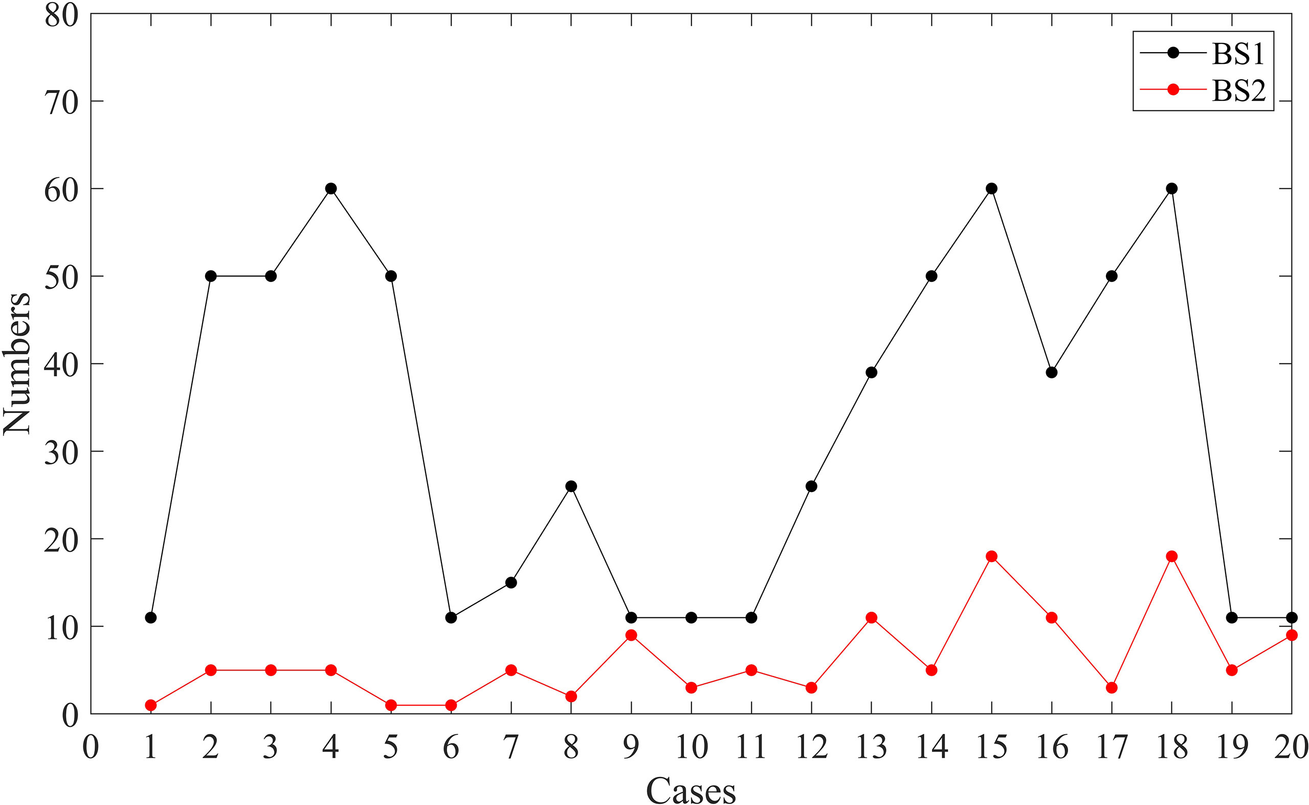
Figure 2 The initial block size BS1 (black dot) and the increment BS2 (red dot) of each cycle for C01-C20.

For cases C02-C05, C13, C15, C17, and C18, since there are many outliers and the distribution of data is relatively concentrated, it is necessary to ensure that there are more good points than outliers in each block when blocks are divided by selecting a large value for BS1 (Figure 2). But it also brings another problem. When we select a large block in a region with a large gradient, the normal variation range is also large, which makes it impossible to accurately detect outliers (Figure 3). Therefore, for case C20, although there are many outliers, most of them are in the region with large gradient. So, a small block size is selected. For cases C01, C06-C12, and C19, there are few outliers, and they are relatively scattered. So a small blocks size is selected. But there are also outliers that cannot be accurately detected in areas with large gradient changes. Even though the outliers of cases C14, C16, and C19 are all detected, other cases have multiple outliers that cannot be detected (Figure 3).

FIGURE 3

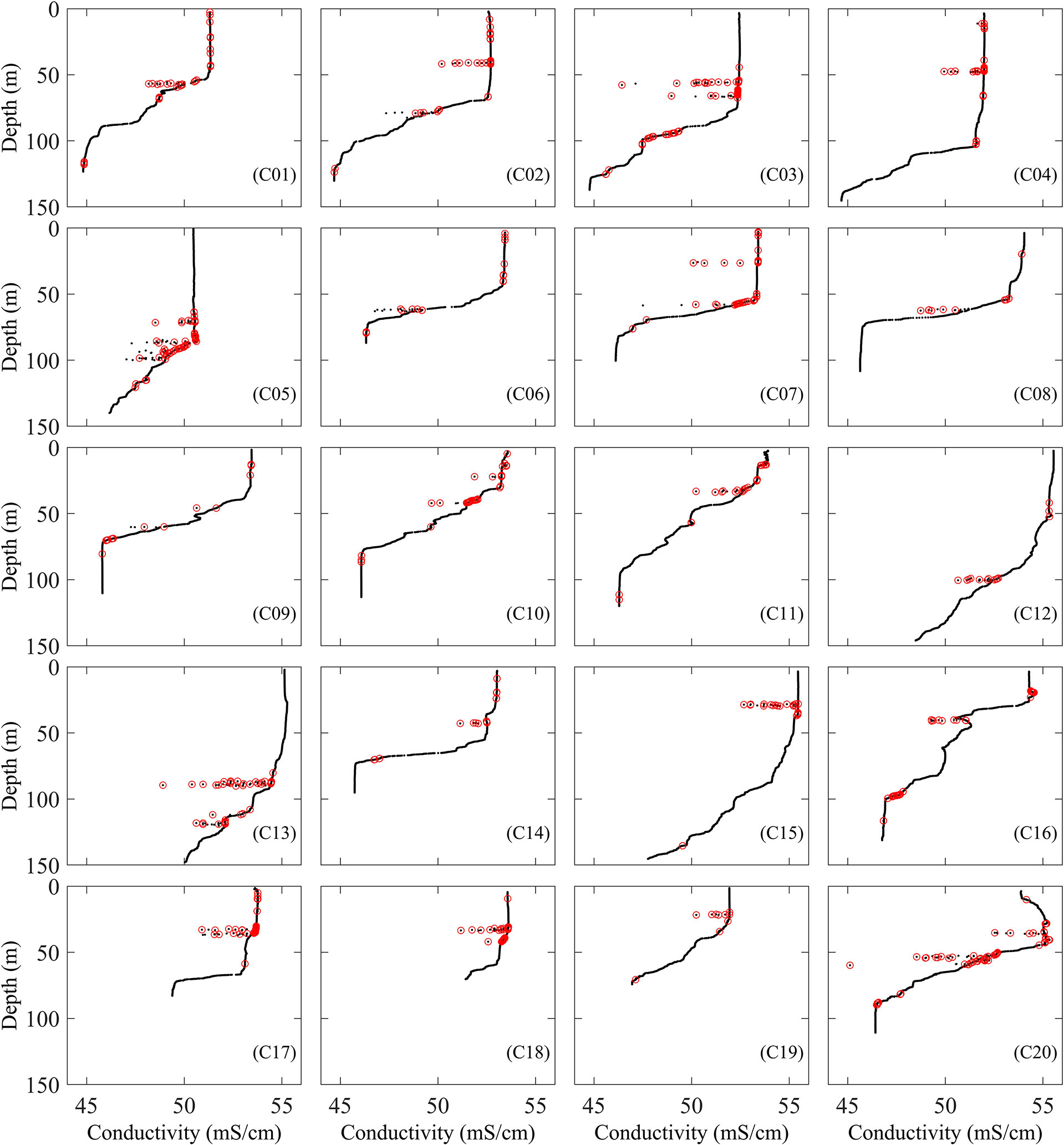
Figure 3 The detected outliers of C01-C20 by the WE method (black points are the original data, and red points are the detected outliers).

In addition, regardless of whether there are outliers ​​in the block, it is inevitable that some good data will be misjudged as outliers, which results in a high false positive rate. This situation exists in C01-C20 (Figure 3).

The WE method is a statistical method based on the PauTa criterion. The results are uncertain and have high false negative and positive rates because the threshold have to be adjusted many times for each case based on experience.

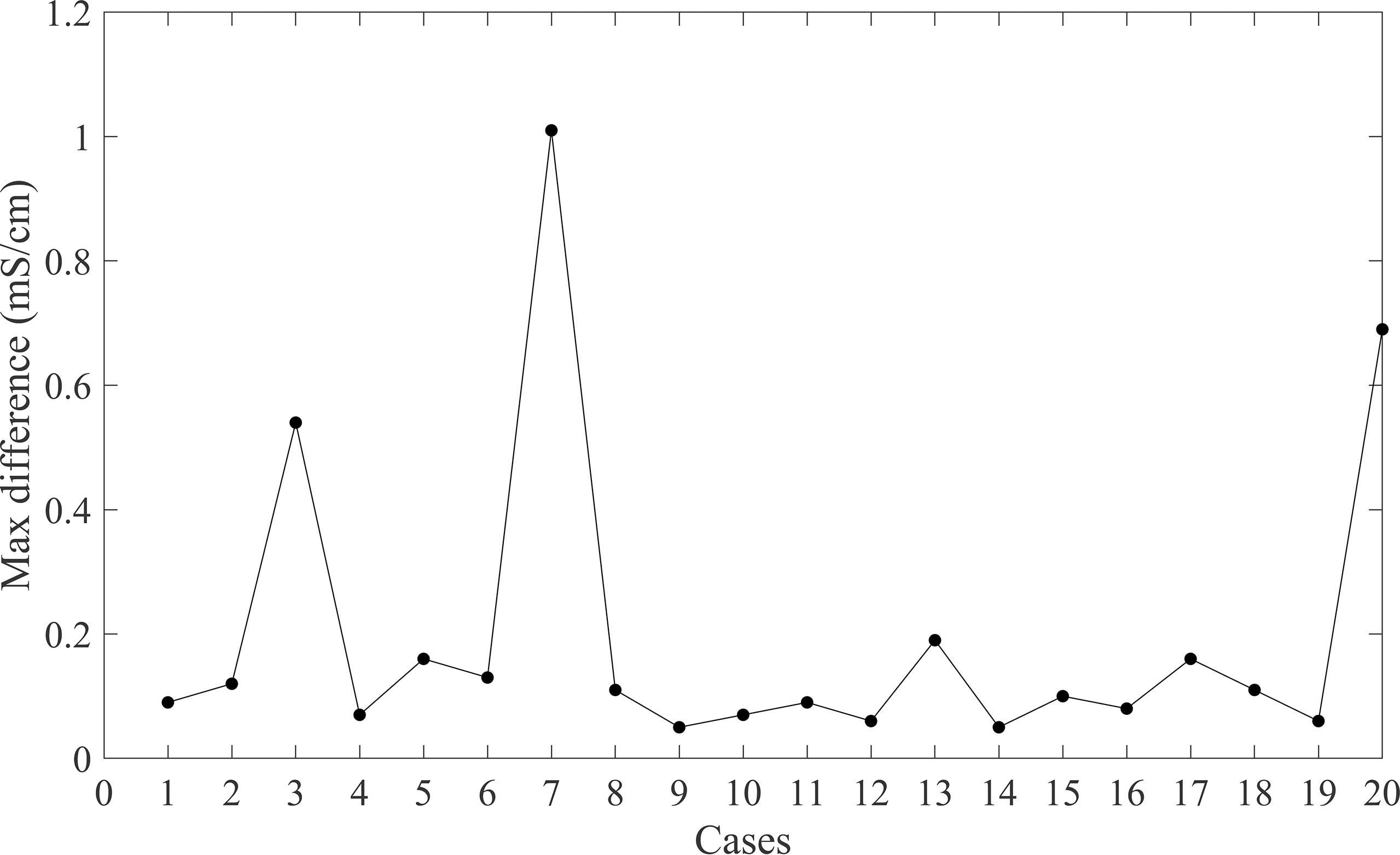
We then applied the MFMD method, and the maximum deviation of each case is shown in Figure 4. Among them, the maximum deviations of C03, C07, and C20 are the largest, i.e. 0.54 mS/cm, 1.01 mS/cm and 0.69 mS/cm respectively. Because there are obvious outliers in the three cases (Figure 1B), the maximum deviation is significantly larger than others, the latter being below 0.19 mS/cm.

FIGURE 4

Figure 4 Maximum conductivity deviation of C01-C20.

The detected outliers of C01-C20 by the MFMD method are shown in Figure 5. For C03, C05, C07 and C20, there are obvious outliers that have not been detected. For C01, C02, C06, C12, C13 and C17, although most outliers are detected, there are still underreports for outliers with small deviations. On the other hand, all the outliers in other cases have been detected. Except for C07, C15, C18 and C20, many cases have a high false positive rate. Especially C08, C09, C10, C14 and C16, which have fewer outliers actually. But the good points with the same number of outliers are misjudged as outliers.

FIGURE 5

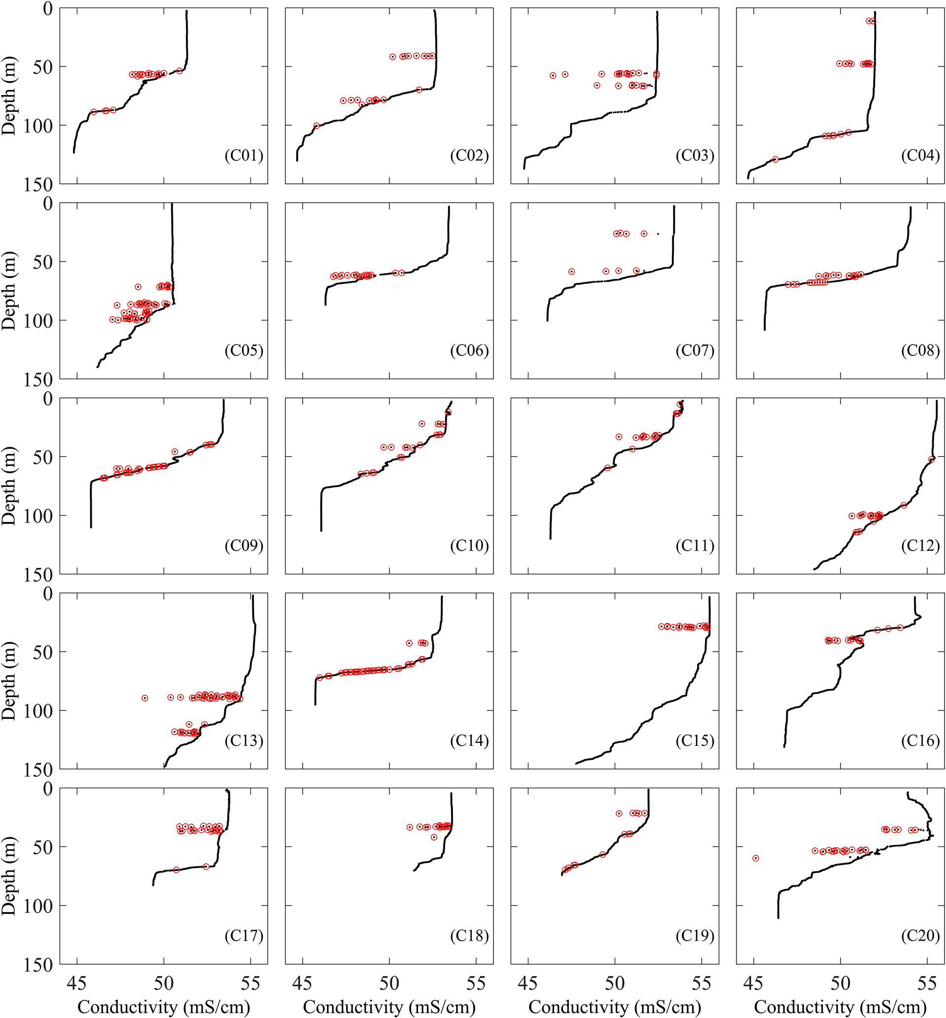
Figure 5 The detected outliers of C01-C20 by the MFMD method (black points are the original data, and red points are the detected outliers).

The MFMD method detects most outliers, but for outliers only slightly differing from good data, it is necessary to set a stricter threshold. If this is not done, the method will cause a higher false positive rate. It is difficult to balance the false negative and positive rate. There is also the uncertainty in the results due to the different threshold selections.

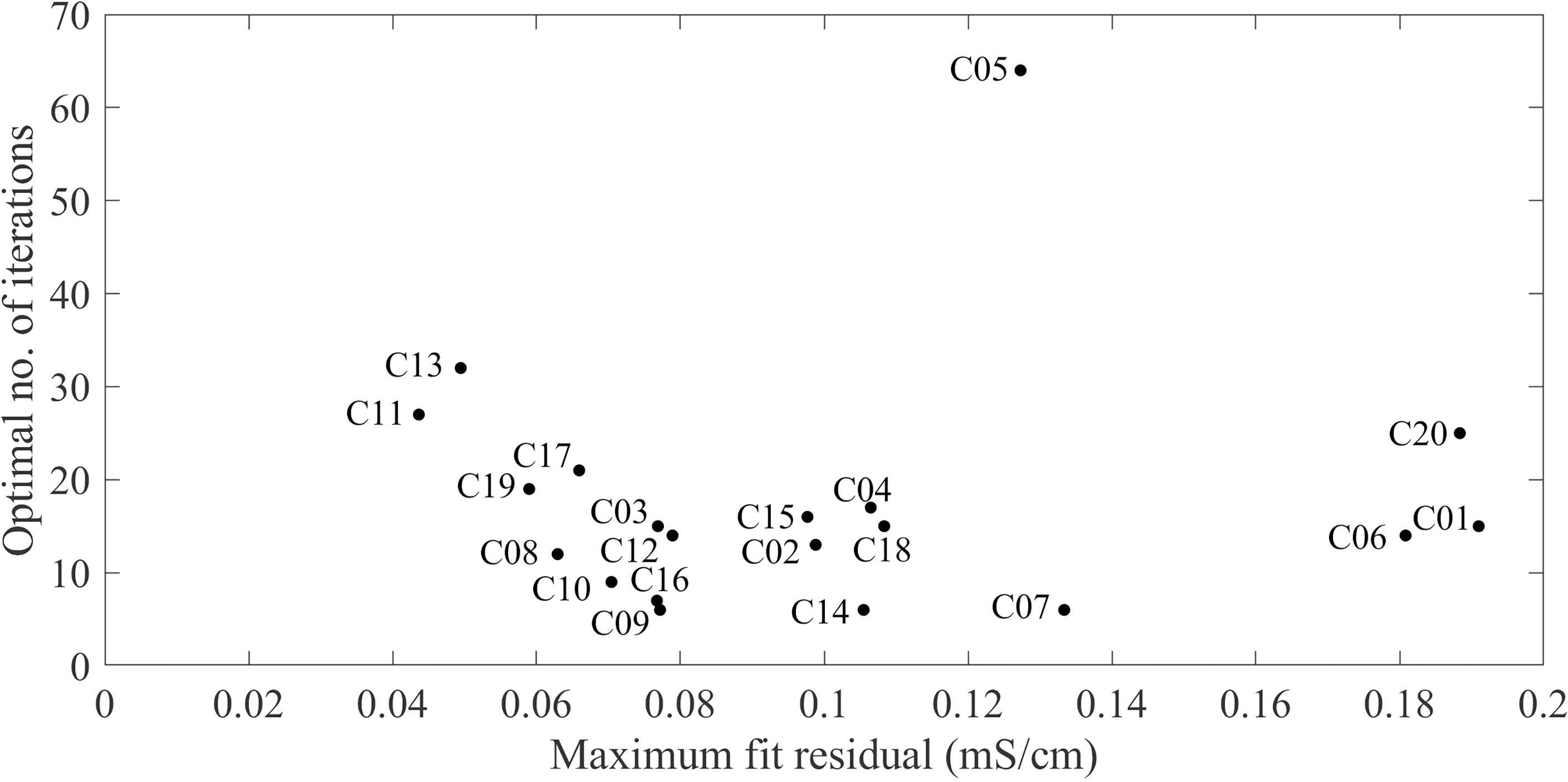
Finally, the CSF method is applied. The optimal number of iterations and corresponding maximum fitting residuals for each case are shown in Figure 6. Among them, the optimal number of iterations for C05 is 64 at most, because the number of outliers of C05 is the largest among all the cases. The optimal number of iterations for C11, C13 and C20 is 27, 32 and 25, respectively, and the optimal number of iterations of other cases is basically below 20. Most of the best fit residuals are in the range of (0.06-0.11) mS/cm. The average number of optimal number of iterations for the 20 cases is 17, and the average maximum fitting residual is 0.1 mS/cm.

FIGURE 6

Figure 6 Optimal number of iterations and corresponding maximum fit residuals for cases C01-C20.

The detection results are shown in Figure 7. Except for C05, C06, C17 and C20, which have a few undetected outliers, the outliers in other cases were detected. There is no false report in C01, C02, C12, and C18, while other cases have few good points that are misjudged as outliers.

FIGURE 7

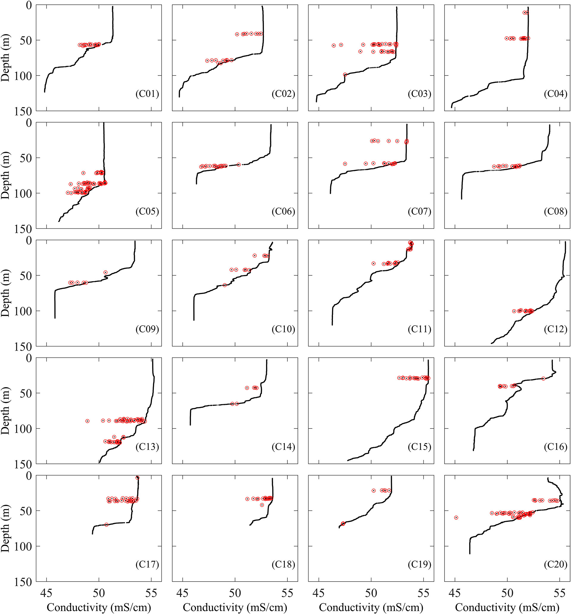
Figure 7 The detected outliers of C01-C20 by the CSF method (black points are the original data, red points are the detected outliers).

Compared with the other two methods, the CSF method can automatically determine the optimal number of iterations, which is simple and effective. It reduces the false negative and positive rate, and the uncertainty of the results is avoided, even though also this method has a certain degree of omission and misjudgment, which may be induced by the original difference between the two conductivity sensors.

The statistical results show that the WE method, the MFMD method and the CSF method have detected 1077, 490 and 492 outliers in these 20 cases respectively. The number of outliers detected by the WE method is significantly higher than the number of outliers detected by the other two methods (Figure 8). The total number of outliers detected by the WE method and the MFMD method are basically the same, but in about half of the 20 cases, there is a big difference in the number of outliers identified by the two methods, such as C02, C04, C06, C11, C15, etc., while in the other half of the cases they are basically the same, such as C01, C03, C08, C12, C16 etc.

FIGURE 8

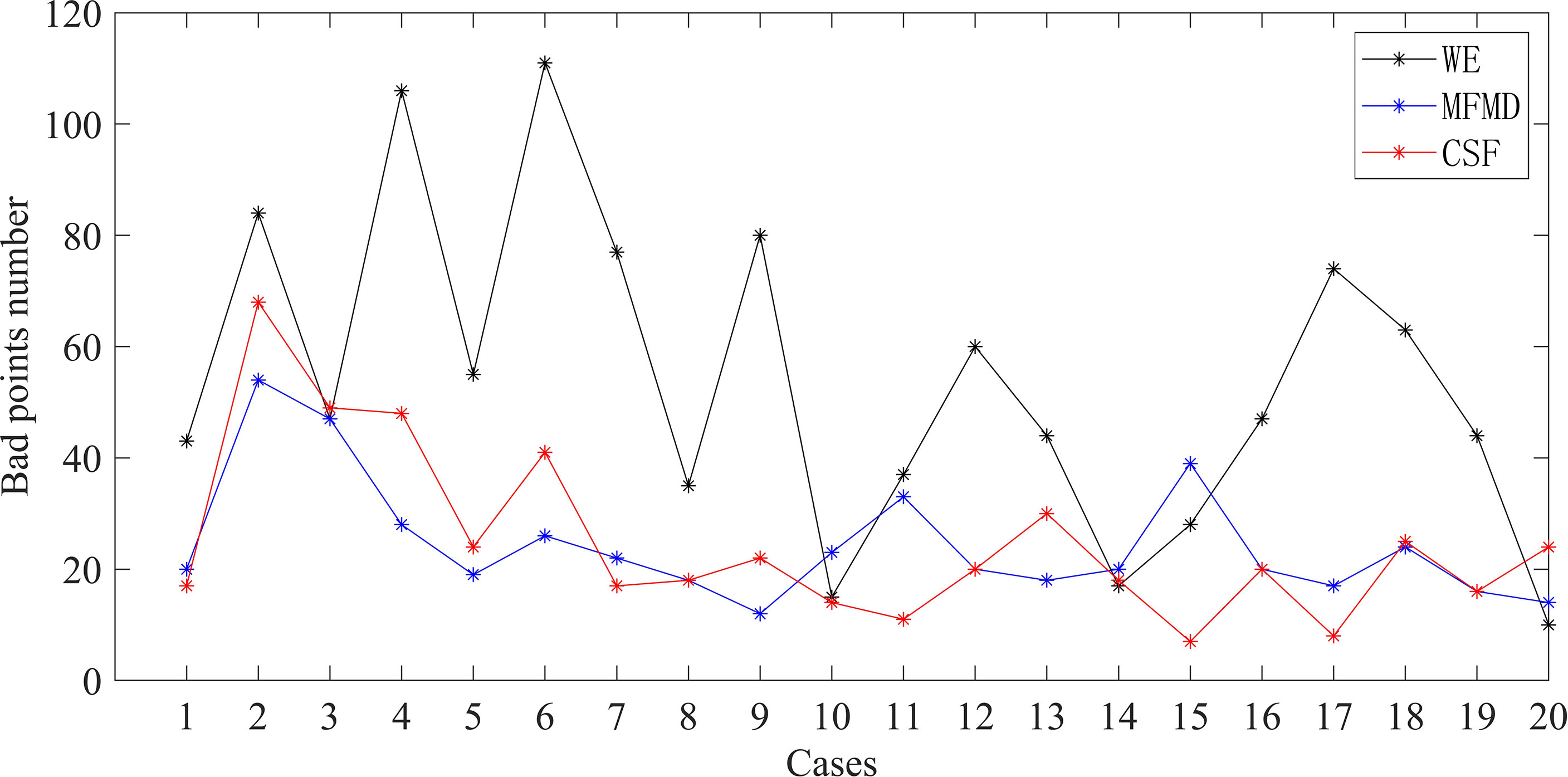
Figure 8 The number of outliers detected by the three methods (the black, blue and red lines represent the number of outliers detected by method WE, MFMD and CSF respectively).

Since the data observed by the second conductivity sensor at the same time are good (Figure 1D), the latter can be used as an important reference for the comparison of the three methods.

We calculate the difference between the data observed by the faulty (Figure 1B) and better working (Figure 1D) conductivity sensor as the discriminant threshold of the outliers, and the relationship between them is shown in Figure 9. When the discriminant threshold is 0.08 mS/cm and 0.12 mS/cm, the rate of change in the number of outliers is about 5% and 1%. In a word, when the discriminant threshold is in the range of (0.08-0.12) mS/cm, the number of outliers keeps stabilized to a minimum value, thus representing the true outliers.

FIGURE 9

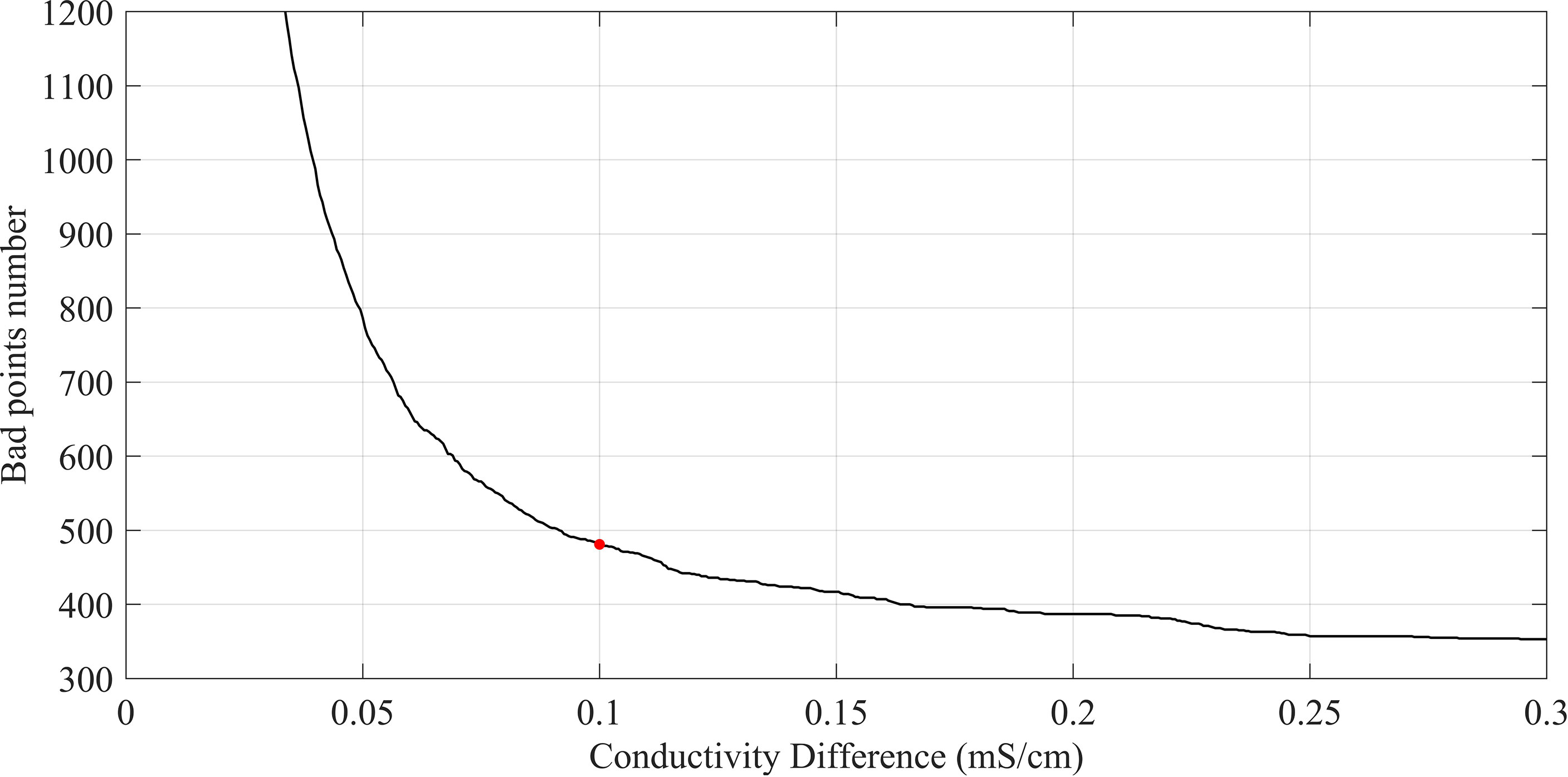
Figure 9 The number of outliers detected by different thresholds applied to the difference between the conductivity data observed by the faulty and better working conductivity sensor.

In order to compare the three methods more clearly, we take the differences between the faulty (Figure 1B) and better working (Figure 1D) conductivity sensor, which is larger than 0.1 mS/cm, as the real outliers. According to the threshold, the number of real outliers is 481 (Red point in Figure 9), while the number of the entire C01-C20 dataset is 40275.

Among the three methods, as shown in Figure 10 and Figure 11, the WE method missed 274 real outliers and misjudged 870 good points as outliers, the false negative and positive rates are 56.96% and 2.19%. The MFMD method missed 113 real outliers and misjudged 122 good points as outliers, the false negative and positive rate are 23.28% and 0.31%. The CSF method missed 86 real outliers and misjudged 97 good points as outliers, the false negative and positive rate are 17.88% and 0.24%.

FIGURE 10

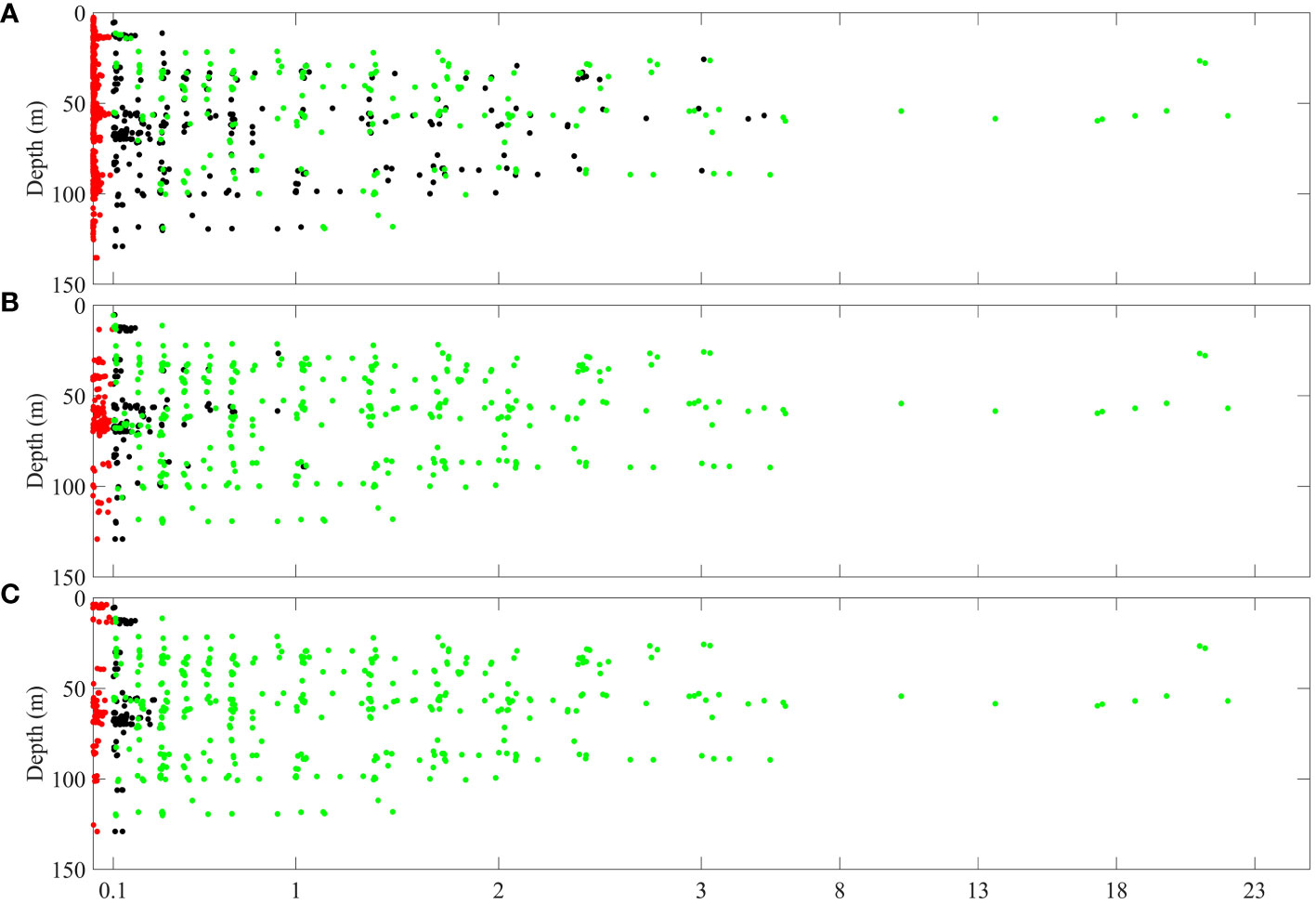
Figure 10 The outliers detected by the three methods in 20 cases. (A-C) are the distribution of outliers detected by the WE method, the MFMD method and the CSF method respectively. Green dots, black dots and red dots are real outliers, missed real outliers, and misjudged good data, respectively.

FIGURE 11

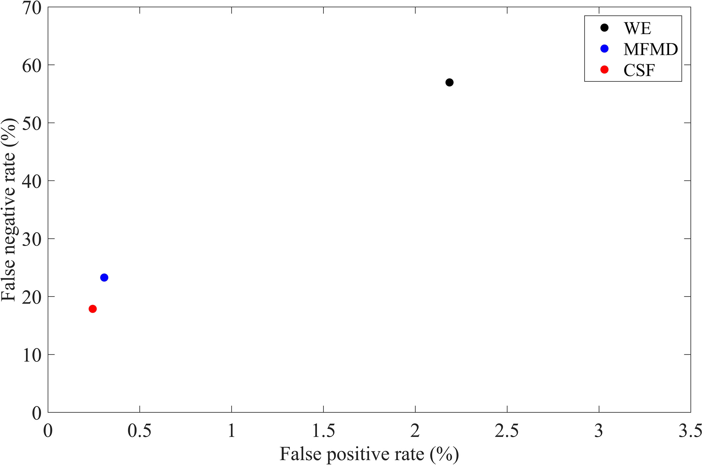
Figure 11 The false negative and positive rate of the three methods (the black, blue and red dots represent the method WE, MFMD and CSF respectively).

4 Conclusion

At present, the detection of outliers in CTD data is mostly based on statistical methods. The outliers are detected by setting a threshold. Values greater than the threshold are treated as outliers, but there is no clear specification for the selection of threshold. The results are uncertain due to the selection of different thresholds, which generally leads to high false negative and positive rates.

In order to solve the above problems, we proposed an outlier detection method in CTD conductivity data, based on the physical constraint of seawater continuity. Curves of physical ocean parameters such as conductivity and temperature at the same location should be continuous and smooth. It is thus possible to construct fitting functions for these measurements and then compare them to the fitting curve. So, we construct a cubic spline fitting function based on the independent points scheme and the cubic spline interpolation to fit the conductivity data. The maximum fitting residual points will be flagged as outliers. The fitting stops when the optimal number of iterations is reached, which is automatically obtained by the minimum value of the sequence of maximum fitting residuals. Verification of the accuracy and stability by means of examples shows that this method has lower false negative rate of 17.88% and false positive rate of 0.24%, while the corresponding Wild Edit method values are 56.96% and 2.19% and Median Filter Combined with Maximum Deviation method are 23.28% and 0.31%. During this process, we also give the reasonable range of conductivity outliers detection threshold (0.08-0.12) mS/cm and the optimal conductivity outliers detection threshold 0.1 mS/cm.

Compared with the Wild Edit method and Median Filter Combined with Maximum Deviation method through a series of comparative experiments, the Cubic Spline Fitting method is simple to operate, effective and the result is clear and definite. This method better solved the problem of conductivity outliers detection, thus it represents is a reliable outlier detection method for CTD data quality control.

Data availability statement

The raw data supporting the conclusions of this article will be made available by the authors, without undue reservation.

Author contributions

XX, XL and FY designed the research. LY, BZ, JS and GY performed the research. LY, BZ wrote the manuscript. YG, LC and XJ analyzed the data. All authors contributed to the article and approved the submitted version.

Funding

This work was supported by the Basic Scientific Fund for National Public Research Institutes of China (Grant No.2020Q05), the Shandong Provincial Natural Science Foundation (Grant No.ZR2022MD020), the National Natural Science Foundation of China (Grant Nos.41706034, 41806123 & 41506034), the National Program on Global Change and Air-Sea Interaction (Grant Nos.GASI-01-TXLL-01 & GASI-04-WLHY-02), the National Science and Technology Major Project (Grant No.2016ZX05057015), Marine Engineering Equipment Research Project (Grant No.CCL2015SKGF0008).

Conflict of interest

The authors declare that the research was conducted in the absence of any commercial or financial relationships that could be construed as a potential conflict of interest.

Publisher’s note

All claims expressed in this article are solely those of the authors and do not necessarily represent those of their affiliated organizations, or those of the publisher, the editors and the reviewers. Any product that may be evaluated in this article, or claim that may be made by its manufacturer, is not guaranteed or endorsed by the publisher.

Supplementary material

The Supplementary Material for this article can be found online at: https://www.frontiersin.org/articles/10.3389/fmars.2022.1030980/full#supplementary-material

References

Balmaseda M. A., Trenberth K. E., K Llén E. (2013). Distinctive climate signals in reanalysis of global ocean heat content. Geophysical Res. Letters. 40 (9), 1754–1759. doi: 10.1002/grl.50382

CrossRef Full Text | Google Scholar

Boyer T. P., Baranova O. K., Coleman C., Garcia H. E., Grodsky A., Locarnini R. A., et al. (2018). “World ocean database 2018,” in NOAA Atlas NESDIS 87 (Silver Spring, Md: Mishonov, Technical Ed).

Google Scholar

Boyer T. P., Levitus S., US Department of Commerce, National Oceanic and Atmospheric Administration (1994). Quality control and processing of historical oceanographic temperature, salinity, and oxygen data. NOAA Technical Report NESDIS. 81, 1–10

Google Scholar

Brunton S. L., Kutz J. N. (2022). Data-driven science and engineering: Machine learning, dynamical systems, and control (Cambridge: Cambridge University Press).

Google Scholar

Bushnell M. (2020). Manual for real-time quality control of in-situ temperature and salinity data: Version 2.1. A guide to quality control and quality assurance of in-situ temperature and salinity observations. U.S. Integrated Ocean Observing System.

Google Scholar

Chen H., Jun L. I., Shuqing M. A., Shuzhen H. U. (2019). Progress of the marine meteorological observation technologies. Sci. Technol. Review. 37, 91–97.

Google Scholar

Davis R. E., Talley L. D., Roemmich D., Owens W. B., Rudnick D. L., Toole J., et al. (2019). 100 years of progress in ocean observing systems. Meteorological Monographs. 59, 1–3. doi: 10.1175/amsmonographs-d-18-0014.1

CrossRef Full Text | Google Scholar

Good S. A., Martin M. J., Rayner N. A. (2013). EN4: Quality controlled ocean temperature and salinity profiles and monthly objective analyses with uncertainty estimates. J. Geophysical Research: Oceans. 118 (12), 6704–6716.

Google Scholar

Gouretski V. (2018). World ocean circulation experiment-argo global hydrographic climatology. Ocean Ence. 14 (5), 1127–1146. doi: 10.5194/os-14-1127-2018

CrossRef Full Text | Google Scholar

Gouretski V., Cheng L. (2020). Correction for systematic errors in the global dataset of temperature profiles from mechanical bathythermographs. J. Atmospheric Oceanic Technology. 37 (5), 841–855. doi: 10.1175/JTECH-D-19-0205.1

CrossRef Full Text | Google Scholar

Gourrion J., Dobler D., Szekely T. (2020). A novel statistical approach for near-real time quality control of hydrographic observations. EGU Gen. Assembly Conf. Abstracts EGU2020–22241. doi: 10.5194/egusphere-egu2020-22241

CrossRef Full Text | Google Scholar

Guo Z., Pan H., Fan W., Lv X. (2017). Application of surface spline interpolation in inversion of bottom friction coefficients. J. Atmospheric Oceanic Technology. 34 (9), 2021–2028. doi: 10.1175/jtech-d-17-0012.1

CrossRef Full Text | Google Scholar

Jiang D., Chen H., Jin G., Lv X. (2018). Estimating smoothly varying open boundary conditions for a 3D internal tidal model with an improved independent point scheme. J. Atmospheric Oceanic Technology. 35 (6), 1299–1311. doi: 10.1175/jtech-d-17-0155.1

CrossRef Full Text | Google Scholar

Jin G., Pan H., Zhang Q., Lv X., Zhao W., Gao Y. (2018). Determination of harmonic parameters with temporal variations: An enhanced harmonic analysis algorithm and application to internal tidal currents in the south China Sea. J. Atmospheric Oceanic Technology. 35 (7), 1375–1398. doi: 10.1175/jtech-d-16-0239.1

CrossRef Full Text | Google Scholar

Liu S. H., Chen M. C., Dong M. M., Gao Z. G., Zhang J. L., Shuang-Quan W. U., et al. (2016). A quality control method for the outlier detection of buoy observations. Mar. Ence Bulletin 35, 264–270.

Google Scholar

Liu S., Chen G., Liu Y., Tian F. (2020). Research and analysis on marine big data applied technology. Periodical Ocean Univ. China. 50 (1), 154–164.

Google Scholar

Lueck R. G. (1990). Thermal inertia of conductivity cells: Theory. J. Atmospheric Oceanic Technology. 7 (5), 741–755. doi: 10.1175/1520-0426(1990)007<0741:TIOCCT>2.0.CO;2

CrossRef Full Text | Google Scholar

Mensah V., Roquet F., Siegelman-Charbit L., Picard B., Pauthenet E., Guinet C., et al. (2018). A correction for the thermal mass–induced errors of CTD tags mounted on marine mammals. J. Atmospheric Oceanic Technology. 35 (6), 1237–1252. doi: 10.1175/jtech-d-17-0141.1

CrossRef Full Text | Google Scholar

Morison J., Andersen R., Larson N., D’Asaro E., Boyd T. (1994). The correction for thermal-lag effects in Sea-bird CTD data. J. Atmospheric Oceanic Technology. 11 (4), 1151–1164. doi: 10.1175/1520-0426(1994)011<1151:TCFTLE>2.0.CO;2

CrossRef Full Text | Google Scholar

Palmer M. D., Roberts C. D., Balmaseda M., Chang Y. S., Chepurin G., Ferry N., et al. (2017). Ocean heat content variability and change in an ensemble of ocean reanalyses. Climate Dynamics. 49 (3), 909–930. doi: 10.1007/s00382-015-2801-0

CrossRef Full Text | Google Scholar

Pan H., Guo Z., Lv X. (2017). Inversion of tidal open boundary conditions of the M2 constituent in the bohai and yellow seas. J. Atmospheric Oceanic Technology. 34 (8), 1661–1672. doi: 10.1175/jtech-d-16-0238.1

CrossRef Full Text | Google Scholar

Roemmich D., Alford M. H., Claustre H., Johnson K., King B., Moum J., et al. (2019). On the future of argo: A global, full-depth, multi-disciplinary array. Front. Mar. Science. 6. doi: 10.3389/fmars.2019.00439

CrossRef Full Text | Google Scholar

Sea-Bird Electronics I. (2013). Seasoft V2: SBE data processing - CTD data processing and plotting software for windows XP, windows vista, or windows 7 (Washington: Sea-Bird Electronics, Inc).

Google Scholar

Sy A. (1983). Warmwassersphäre: Handling and processing of hydrographic data (Technical report, Beichte aus dem Institut für Meereskunde, Kiel) 111.

Google Scholar

Tan Z., Zhang B., Wu X., Dong M., Cheng L. (2021). Quality control for ocean observations: From present to future. Sci. China. Earth Sci. 65 (2), 215–233. doi: 10.1007/s11430-021-9846-7

CrossRef Full Text | Google Scholar

Thomson R. E., Emery W. J. (2014). Data analysis methods in physical oceanography (Newnes: Digital Filters) 80 (9), 593–637.

Google Scholar

Wang Y., Pan H., Wang D., Lv X. (2019). A methodology for fitting the time series of snow depth on the Arctic Sea ice. J. Atmospheric Oceanic Technology. 36 (8), 1449–1462. doi: 10.1175/jtech-d-18-0093.1

CrossRef Full Text | Google Scholar

Wong A., Keeley R., Carval T. (2021). Argo quality control manual for CTD and trajectory data. Argo Data Management team. doi: 10.13155/33951

CrossRef Full Text | Google Scholar

Wu X., Zhou H., Cao M., Liu Z., Sun C., Lu S. (2019). Preliminary quality discussion between ship-based CTD and profiling floats observational data. Oceanologia et Limnologia Sinica. 50 (2), 278–290. doi: 10.11693/hyhz20180400099

CrossRef Full Text | Google Scholar

Xu J. P., Su J. L. (1999). Simple analysis of the qualitative control for CTD data. Acta Oceanologica Sin. 21 (1), 126–132.

Google Scholar

Xu M., Wang Y., Wang S., Lv X., Chen X. (2021). Ocean tides near Hawaii from satellite altimeter data. part I. J. Atmospheric Oceanic Technology. 38 (5), 937–949. doi: 10.1175/JTECH-D-20-0072.1

CrossRef Full Text | Google Scholar

Yang Y., Miao Q., Wei G., Dong M., Dong C. (2017). Quality control methods and application for the oceanic station observed data in the delayed mode. Ocean Dev. Management 34, 109–113.

Google Scholar

Yu R. C., Lü S. H., Qi Y. Z., Zhou M. J. (2020). Progress and perspectives of harmful algal bloom studies in China. Oceanologia et Limnologia Sinica 51 (4), 768–788.

Google Scholar

Zhang J., Chu D., Wang D., Cao A., Lv X., Fan D. (2018). Estimation of spatially varying parameters in three-dimensional cohesive sediment transport models by assimilating remote sensing data. J. Mar. Sci. Technology. 23 (2), 319–332. doi: 10.1007/s00773-017-0477-3

CrossRef Full Text | Google Scholar

Zhang B., Fan W., Cheng L., Xin W., Zhang D., Yuan Z., et al. (2017). Observation data processing method and product development of key parameters of marine environmental change. China Basic Science 19, 6–11.

Google Scholar

Zong X., Pan H., Liu Y., Lv X. (2018). Improved estimation of pollutant emission rate in an ocean pollutant diffusion model by the application of spline interpolation with the adjoint method. J. Atmospheric Oceanic Technology. 35 (10), 1961–1975. doi: 10.1175/jtech-d-17-0208.1

CrossRef Full Text | Google Scholar

Zou L., Zhou T., Tang J., Liu H. (2020). Introduction to the regional coupled model WRF4-LICOM: Performance and model intercomparison over the Western north pacific. Adv. Atmospheric Sci. 37 (8), 800–816. doi: 10.1007/s00376-020-9268-6

CrossRef Full Text | Google Scholar