A Seasonal Undercurrent Along the Northwest Coast of Australia

In the North West Shelf region of Australia is a surface current (Holloway Current), which flows southwestward along the shelf break. This paper describes a seasonal undercurrent below the Holloway Current. A 5-day climatology is constructed from the output of an eddy-resolving oceanic general circulation model (OGCM). A seasonal northeastward-flowing undercurrent is found on the upper continental slope during the climatological April–May. This undercurrent reverses during February–March. During its annual cycle, the phase of the undercurrent tends to propagate southwestward and upward. The annual frequency dominates, but the positive and negative phases of the undercurrent are not symmetric in the yearly cycle because of the contributions from the semi-annual and 1/3-annual components. We propose a hypothesis that this undercurrent is a beam of coastal trapped wave (CTW). As an initial attempt to assess the plausibility of this hypothesis, we construct an idealized linear coastal-trapped wave (CTW) solution driven by an idealized harmonic meridional winds at the annual frequency. The solution takes the form of a beam originating from the forcing region on the continental shelf and propagating offshore and southward. When it emerges on to the continental slope, it takes the form of an undercurrent. This idealized solution shares several properties with the undercurrent in the OGCM despite several discrepancies.

1. Introduction

Along the northwest and west coasts of Australia flow several coastal currents [see the review paper by Phillips et al. (2021) and references therein]. The Leeuwin Current flows poleward along the west coast; it is a permanent current with well known annual variability. One of the sources of this surface current is the Holloway Current (D'Adamo et al., 2009), which flows southwestward along the shelf break in the North West Shelf region of Australia and extends from the sea surface to ~100 m (Brink et al., 2007; Marin and Feng, 2019). It is strongest during austral autumn (D'Adamo et al., 2009; Bahmanpour et al., 2016; Katsumata and Ridgway, under review). Marin and Feng (2019) examined the semi-annual and intraseasonal variabilities of the Holloway Current and reported that the variabilities are consistent with the propagation of 2nd-mode and 1st-mode coastal trapped waves, respectively.

Below the Leeuwin Current along the west coast, there is a well known equatorward undercurrent, called the Leeuwin Undercurrent (LUC), which hugs the continental slope and extends from 200 to 800 m (e.g., Furue et al., 2017). In the annual average, the LUC leaves the continental slope, veering offshore westward or northwestward (Duran, 2015; Furue et al., 2017). Its annual variability, if any, is not known.

The vertical structure of the coastal currents on the northwest coast is not well known either. One of Brink et al.'s (2007) hydrography-based longshore velocity plots during mid-June to mid-July shows a subsurface core of northeastward (opposite to the surface current) velocity hugging the continental slope (their Figure 4). Bahmanpour et al.'s (2016) monthly-mean mooring data shows a hint of a subsurface counter flow during May (their Figure 4). A plot from a high-resolution numerical model of Marin and Feng (2019) sometimes shows a similar subsurface counter flow (their Figure 12). One potential mechanism to cause an undercurrent is Kelvin waves or coastal trapped waves (e.g., McCreary, 1981a; Samelson, 2017). For the Leeuwin Current, the poleward advection of lighter water by the surface current can cause an equatorward undercurrent by thermal wind shear (Benthuysen et al., 2014; Schloesser, 2014). This type of undercurrent sits above or in the upper part of the pycnocline.

1.1. Coastal Trapped Waves and Kelvin Waves

Pressure disturbances near the coast in a stratified ocean away from the equatorial region propagate along the coast as coastal Kelvin waves or coastal trapped waves. Since these waves propagate vertically as well as along the coast, they can drive oscillatory undercurrents (Nethery and Shankar, 2007).

The terminology is often confused but here in this paper, we call those waves strongly affected by the bottom slope “coastal trapped waves (CTWs)” and the other, simpler type on which the bottom slope has negligible impacts, the coastal “Kelvin waves” (Wang and Mooers, 1976; Hughes et al., 2019).

Both types of wave are trapped to the coast or to the continental shelf and slope and propagate with the coast on their left hand side in the southern hemisphere (e.g., Gill, 1982, section 10.4, for Kelvin wave; e.g., Brink, 1991, for CTW). They are often viewed as a superposition of “modes,” each with a fixed crossshore–depth structure and a phase speed of longshore propagation depending on the background stratification and bottom topography (e.g., McCreary, 1981b, for Kelvin wave; e.g., Brink, 1991, for CTW). A typical phase speed of the gravest “baroclinic” mode is ~2–3 m/s around Australia (e.g., Chelton et al., 1998, for Kelvin wave; e.g., Church et al., 1986a, for CTW), the speed of CTW strongly depending on the bottom topography.

A number of past studies on Australian coastal currents utilized a linear CTW formulation (see section 2.3 below). For example, Church et al. (1986a,b), Freeland et al. (1986), Merrifield and Middleton (1994), and Maiwa et al. (2010) examined velocity data from mooring arrays or numerical models on the continental shelf and slope of the east coast or south coast of Australia and found that some fraction of the variability over time scales of ~10 d agrees with theoretical CTW modes (section 2.3 below). At intraseasonal to annual time scales, Ridgway and Godfrey (2015) and Marin and Feng (2019) examined observed variability of sea-level anomaly and longshore velocity anomaly, respectively, and interpreted them as propagation of CTWs.

1.2. Trapping to the Boundary

When the Coriolis parameter varies in the longshore direction (the planetary beta effect), the Kelvin waves on the eastern side of the basin propagate westward away from the coast as a Rossby wave and do not take the form of a trapped wave when the frequency of the wave is lower than a crtical frequency, that is, when ω < c_jβ cos θ/(2|f|), where ω is the frequency of the Kelvin wave, c_j is the phase speed of gravity wave for the jth vertical mode, and θ is the angle the coast line makes with due north (Clarke and Shi, 1991). For each given frequency, we often express this result in terms of the “critical latitude,” which is the latitude y_c that satisfies ω = c_jβ(y_c) cos θ/[2|f(y_c)|]. For example, the 1st-mode Kelvin wave at the annual frequency is trapped to the coast only poleward of 50° or 40° for a meridional or 45°-slanted coast line, assuming that c₁ ≈ 3 m/s, which is a typical value offshore of the northwest coast of Australia (Chelton et al., 1998). For this reason, coastally-trapped low frequency flows can exist in a flat-bottom ocean only when dissipation arrests high-order modes (e.g., McCreary, 1981a) or when mesoscale eddies trap the flows (Cessi and Wolfe, 2013).

When the continental shelf and slope are influential, however, there is no clear answer as to whether or not CTWs remain trapped to the coast equatorward of the critical latitude. To the best of my knowledge, there has not been analytic solutions to the linearized system (described in Appendix A) with planetary beta except for a steady-state solution discussed below. Clarke and Gorder (1994) considered the poleward propagation of ENSO signal with bottom topography in numerical solutions to the linear system and concluded that friction is necessary for the signal to be trapped to the eastern boundary equatorward of the critical latitudes of the ENSO frequencies. It is, however, not clear whether or not coastal trapped signals remain without friction when they are generated at the coast. Samelson (2017) developed a theory of how low-frequency variability propagates poleward as a CTW along an eastern boundary and part of their energy leaves the coast as planetary Rossby waves. Furue et al. (2013) obtained analytic solutions of inviscid steady flow trapped to the continental slope along the eastern boundary to a $1\frac{1}{2}$-layer system on a beta plane, demonstrating that inviscid longshore steady flow can exist thanks to the topographic beta of the slope.

1.3. Coastal Undercurrents

A pair of a surface equatorward current and subsurface poleward flow along an eastern boundary is a ubiquitous feature for eastern-boundary upwelling systems (e.g., Samelson, 2017). In the South Indian Ocean, a similar pair is found, the Leeuwin Current and the Leeuwin Undercurrent, but with opposite signs: the surface and subsurface currents flow poleward and equatorward, respectively. This difference is because it is a downwelling regime due to the strong surface steric gradient (Thompson, 1984, 1987; Godfrey and Ridgway, 1985).

In McCreary's (1981a) solutions in an flat-bottom ocean, not only the currents are trapped to the coast as stated above but also they form a baroclinic pair similar to the observed flows along the eastern boundary. This mechanism requires perhaps unrealistically large vertical mixing and also the lateral boundary conditions for this flat-bottom model may not be realistic in the presence of the continental shelf and slope (Samelson, 2017).

Samelson (2017) proposes an inviscid model that produces a pair of steady coastal currents along the eastern boundary similar to observation. This solution is constructed by matching a fast CTW response on an f plane on the continental shelf with a slow quasi-geostrophic response on a β plane on the continental slope.

1.4. Present Study

In this study, we construct a 5-day climatology from a 25-year output of an eddy-resolving OGCM and describe a seasonal undercurrent trapped to the continental slope of the North West Shelf region of Australia. We propose a hypothesis that this undercurrent is a beam of CTW. As an initial attempt to assess the plausibility of this hypothesis, we construct a solution to an idealized linear CTW model on an f plane, which shows an undercurrent that has some similarity to the undercurrent in the OGCM.

The rest of this paper is structured as follows. The next section (section 2) describes the OGCM data and an observational dataset, presents the methods of analysis, and then briefly describes the idealized CTW model; details of the model are found in Appendix A. The appendix also discusses some salient properties of the idealized solution which are not directly relevant to the comparison with the OGCM.

Section 3 first describes the seasonal undercurrent. The dominant temporal Fourier components are then examined to elucidate the temporal-spatial characteristics of the flow and the propagation of the signals at the dominant frequencies. The section then shows solutions to the idealized linear model and discusses its similarities to, and differences from, the undercurrent in the OGCM. Section 4 finally summarizes the results and discusses them for potential future extensions of the present study. Supplementary Material records minor details of the methods and also includes figures which are not essential to this paper but can be useful to the interested reader.

2. Data and Methods

2.1. Data

2.1.1. OGCM

Details of our model, called OFES2, are found in Sasaki et al. (2020) and the data is available from the OFES homepage¹. The model domain extends from 76°S to 76°N; the model's resolution is 1/10° horizontally and it has 105 levels in the vertical with 55 levels in the upper 500 m. It is a variant of MOM3 (Pacanowski and Griffies, 2000) with a parameterization of vertical mixing based on St. Laurent et al. (2002) and a mixed layer parameterization of Noh and Kim (1999) and is driven by sea-surface fluxes of momentum, heat, and salt determined using the bulk formulae of Large and Yeager (2004) on the basis of re-analysis product called JRA55-do (Tsujino et al., 2018).

The bottom drag coefficient is 2.5 × 10⁻³ (nondimensional). The coefficients of lateral biharmonic viscosity and diffusivity vary latitudinally with the cube of the zonal grid spacing (Smith et al., 2000) and are 27 × 10⁹ and 9 × 10⁹ m⁴/s at the equator, respectively (Masumoto et al., 2004). Only the upper 800 m is processed to save computational time (The deepest model layer included spans from about 750 m to 784 m, but we use “800 m” as a nominal lower limit for convenience). This depth range was chosen to accommodate both the Leeuwin Current (0–200 m) and the Leeuwin Undercurrent (200–800 m; Furue et al., 2017).

The ouptputs are daily snapshots, from which we construct a 5-day or pentad climatology over the 25-years of 1992–2016. Although the actual mean length of a year is slightly longer than 365 d, we compress the time axis and treat the mean year as 365 d. There are 73 pentads in the climatological year and the pentad data are defined at the center of each pentad. Details are found in Supplementary Material. This data analysis is inspired by Ridgway and Godfrey (2015), who show a set of monthly plots from a climatological sea level to infer the propagation of coastal trapped waves around Australia. Their plots, however, suggest that to see details of the propagation, the temporal resolution would have to be much higher than monthly. In the present study, we choose a 5-day climatology because 1) as can be seen below, a 5-day interval well resolves the propagation of CTWs, 2) 73, 5, and 1 are the only natural numbers that divide 365 evenly, and 3) 5-day climatology would require much less storage and processing time than 1-day climatology.

We also apply the standard temporal Fourier expansion on the climatological data. For completeness, we record the formalism of the Fourier expansion we use in Supplementary Material.

2.1.2. CARS Aus8

For comparison with OFES2, we use a gridded climatological dataset, called CARS Aus8, of temperature and salinity. It is a 1/8° version of CARS (Dunn and Ridgway, 2002; Ridgway et al., 2002). Hydrographic profiles, including Argo, up to the end of 2012 are included in the production of the product². Thanks to the many high-resolution crossshore profiles that are also included (Ridgway et al., 2002), CARS Aus8 resolve the signatures of narrow coastal currents such as the Leeuwin Current (LC) and Leeuwin Undercurrent along the west coast of Australia (Furue et al., 2017) and the Leeuwin Current Extension (LCE) and Zeehan Current (ZC) along the south coast of Australia and the west coast of Tasmania (Duran et al., 2020). The climatological dataset includes annual mean, annual harmonic, and semi-annual harmonic. The timeseries reconstructed from these three components are shown to be generally consistent with other in-situ observations for the near surface coastal currents (LC, LCE, ZC, etc.) mentioned above (Furue et al., 2017; Duran et al., 2020).

2.2. Methods

2.2.1. Rotation of Coordinates

To simplify the analysis and discussion of the flow along the northwest coast of Australia, we introduce a coordinate system which is rotated clockwise by 45° (Figure 1), inspired by Katsumata and Ridgway (under review). Here we treat the longitude-latitude coordinates as if they were Cartesian and then the transformation is simply

$\begin{array}{ll}\left[\begin{array}{c}{x}^{\text{r}}-x_{\text{o}}\\ y^{\text{r}}-y_{\text{o}}\end{array}\right]\equiv \left[\begin{array}{cc}cos45^{°}& -sin45^{°}\\ sin45^{°}& cos45^{°}\end{array}\right]\left[\begin{array}{c}x-x_{\text{o}}\\ y-y_{\text{o}}\end{array}\right],& (1)\end{array}$

FIGURE 1

Figure 1. Bottom topography from the OGCM (shading), the 200-m isobath (red curve with dots), and the rotated coordinates. See the text for the explanations of the latter two. The numbers along the y^r axis are the values of y^r. This map is plotted in such a way that longitudinal and latitudinal intervals have the same lengths on the paper, so that the rotated y axis makes 45° on the paper.

where x and y are the original longitude and latitude, x^r and y^r are the rotated longitude and latitude, and (x_o, y_o) ≡ (113.85°E, 21.95°S) is the pivot of the rotation. The pivot is the location of the 200-m isobath (see section 2.2.2) at 22°S. Note that the two coordinate system shares the pivot (x_o, y_o) in that (x, y) = (x_o, y_o) implies $(x^{\mathrm{\text{r}}},y^{\mathrm{\text{r}}})=(x_{\mathrm{\text{o}}},y_{\mathrm{\text{o}}})$ according to (1). The rotated latitude is marked in Figure 1 along the y^r axis through the pivot.

We sometimes use a notation like 18°S^r to denote y^r = −18°, for example. The relation between this rotated latitude and the real latitude is obtained along the $x^{\mathrm{\text{r}}}=x_{\mathrm{\text{o}}}$ axis by solving (1) for y when $x^{\mathrm{\text{r}}}=x_{\mathrm{\text{o}}}$, as $y=y_{\mathrm{\text{o}}}+(y^{\mathrm{\text{r}}}-y_{\mathrm{\text{o}}})/\sqrt{2}.$

When the original points (x, y) form a square grid (where Δx = Δy), the transformed points (according to formula 1) are shown to also form a square grid with $\Delta x^{\mathrm{\text{r}}}=\Delta y^{\mathrm{\text{r}}}=\Delta x/\sqrt{2}$. The original gridpoints fill only half of the x^r-y^r gridpoints. The remaining half are determined by horizontal interpolation.

We accordingly define rotated velocity components u^r and v^r and, for simplicity, call v^r the “longshore velocity” in the North West Shelf region (defined in this paper as equatorward of 22°S). In the west coast region, v is called the longshore velocity. When discussing the flow field along the northwest coast, we say “northeastward” and “southwestward” for longshore directions.

2.2.2. 200-m Isobath

As a reference of analysis, we define a curve that approximately follows the 200-m isobath (red curve in Figure 1). We first locate the scalar gridpoints of the model whose depths are closest to 200 m [Since the model uses partial bottom cells (Pacanowski and Griffies, 2000), the model's topography is as close to the real one at the given horizontal resolution]. We then manually remove points in such a way as to ensure that only one point exists for each y along the west coast (poleward of 22°S) or for each y^r along the northwest coast (equatorward of 22°S).

Along the west coast of Australia, this manual procedure was not necessary because the 200-m isobath is relatively regular and largely oriented north–south. Along the northwest coast, in contrast, the 200-m isobath is complex (Figure 1), necessitating some manual removal. In particular, the removal of the concave shapes of the 200-m isobath at about 123°E, 13°S and 125°E, 12°S result in large jumps in $x_{\mathrm{\text{c}}}^{\mathrm{\text{r}}}(y^{\mathrm{\text{r}}})$; see the jumps in the red curve in the x^r direction northeast and southwest of y^r = −8° in Figure 1.

As will be seen below, the main currents focused on in this paper exist around ~150 m depth but we still choose the 200-m isobath as a reference because this isobath is more “stable” along the northwest coast. Shallower isobaths migrate wildly in the crossshore direction and are not always representative of the inshore edge of the continental slope.

To represent the flow along and on the continental slope, we take average between $x_{\mathrm{\text{c}}}^{\mathrm{\text{r}}}-$0.5° and $x_{\mathrm{\text{c}}}^{\mathrm{\text{r}}}+$0.2° as this is a typical width of the current we analyze below. For convenience, we call this averaging band the “x_c strip.”

2.3. Linear Coastal-Trapped-Wave Model

To compare with the OFES2 results, we use an idealized linear model for coastal trapped waves (CTWs). In this section, we present only an outline of the model and its configuration; details are found in Appendix A. The original formalism is developed in a series of papers including Brink and Allen (1978) and Brink (1982b); the formalism is summarized and comprehensively discussed in Clarke and Brink (1985) and a concise summary is found in the appendix of Church et al. (1986a).

For this model, we take y to be the longshore (northeastward) coordinate, x ≤ 0 to be the crossshore (southeastward) coordinate with x = 0 at the lateral boundary, and z to be the vertical. We assume a horizontally-uniform background density stratification and linearize the primitive equation around the state of no motion with this stratification; we further make the “long-wave” assumption (Appendix A). We ignore friction for simplicity; potential impacts of friction are briefly discussed in section 4.3. We consider curl-free longshore winds only and assume that the Coriolis parameter is uniform.

Then, the set of equations has coastally-trapped wave solutions in the form of

$\begin{array}{ll}p={\displaystyle \sum _j}{F}_j(x,z){\varphi }_j(y,t),& (2)\end{array}$

where ϕ_j is the solution to

$\begin{array}{ll}\left[-(1/c_j){\partial }_t+{\partial }_y\right]{\varphi }_j=b_j{\tau }^y(y,t).& (3)\end{array}$

The solution to the latter equation is a wave that is forced by τ^y and propagates in the negative y direction at a speed of c_j > 0. The “coupling coefficient” b_j, determined by the shape of the “mode” F_j(x, y), represents how strongly the wind forces mode j. The “modes” F_j are the solutions to a two-dimensional eigenvalue problem, which depends on the background stratification N(z) and the bottom profile z = −h(x); and c_j are the corresponding eigenvalues.

We numerically solve this eigenvalue problem using Brink and Chapman's (1987) Fortran program, whose latest version (updated in 2007) is available from https://www.whoi.edu/cms/files/Fortran_30425.htm, with a representative background stratification and a smoothed bottom topography of a part of the northwest coast of Australia (Appendix A). The maximum depth is set to 2,000 m.

We use 90 gridpoints in the vertical. The horizontal (in x) gridspacing is about 6.6km, there are 100 gridpoints in x, and h(x) reaches the prescribed maximum depth (2,000m) at x ≈ −390 km. The artificial offshore boundary (x ≈ −660 km) is sufficiently far from this bottom edge (x ≈ −390 km) of the continental slope for all the coastal modes to sufficiently decay until the artificial boundary is reached (Figure A2 in Appendix), a necessary condition for the accuracy of the calculated modes (Brink and Chapman, 1987). We obtain modes 1–24, all of which are sufficiently resolved both in the horizontal and vertical (Figure A2 in Appendix).

We will use a simple oscillatory wind τ^y ∝ e^ιωt at a given frequency over a limited latitude range L > y > 0, calculate the y-t structure of the response of each mode according to (3), and obtain the total solution as a superposition of the modes according to (2).

The original CTW model is somewhat more general (Appendix A.4) than described above but we make the simplifications as our aim of using this model is not a quantitative comparison with the OGCM flow field but a qualitative interpretation of the latter without huge quantitative disagreement.

3. Results

3.1. Horizontal Structure

Figure 2 shows the mean flow for the “surface” (0–200 m) and “subsurface” (200–800 m) layers.

FIGURE 2

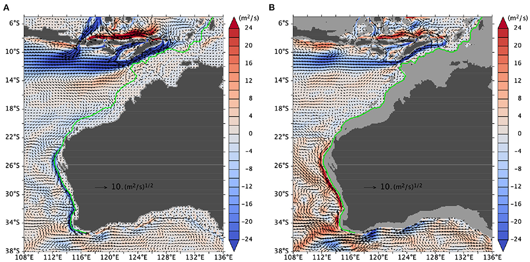
Figure 2. Mean flow vertically integrated (A) over 0–200 m and (B) over 200–800 m from OFES2. The color shading shows the “longshore” component of the transport vector, that is, V poleward of 22°S and V^r equatorward of it. To reduce the clutter, the arrows are scaled by the square root of the length: U/|U|^1/2. The green curve approximately follows the 200-m isobath (section 2.2.2).

From mid March through May, the southwestward-flowing Holloway current is clearly seen (not shown) along or near the shelf break of the North West Shelf region. This seasonality agrees with D'Adamo et al.'s (2009) description. The current's annual mean (Figure 2A) is similar to that of Marin and Feng (2019) (Supplementary Material). As noted in the introduction, the mean Leeuwin Undercurrent (LUC) leaves the coast of Australia at 22°S and flows westward or northwestward in a broad current. That is also the case for OFES2 (Figure 2B).

During the annual cycle, however, the undercurrent appears to extend to 13°S along the coast during May 8 to July 12 (Figure 3). On closer examination, there is a coastal branch for this undercurrent, which peaks around May 13 (Figure 3). Shortly after this peak, an offshore branch intensifies and peaks around June 17 (not shown). As will be shown below, the inshore branch of the undercurrent is a narrow longshore flow hugging the continental shelf just below the shelf break on the northwest coast. The profile of the continental shelf and continental slope varies much more than along the west coast but the shelf break is systematically shallower just below at 100 m. For this reason, the vertical averages for the upper and lower layers for Figure 3 are separated at 100 m.

FIGURE 3

Figure 3. Velocity anomaly (pentad annual cycle minus annual mean) vertically integrated (A) over 0–100 m and (B) over 100–800 m on May 13. For this plot, the division between the upper and lower layers is at 100 m, as the separation between the surface current and the undercurrent is located roughly at this depth. See text. To reduce the clutter, the arrows are scaled by the square root of the length: U/|U|^1/2. The green curve approximately follows the 200-m isobath (section 2.2.2).

Figure 4 compares density anomaly between CARS and OFES2. It is interesting that there is a very thin strip of density anomaly along the continental slope of the northwest coast (Figure 4A). The overall pattern of density anomaly is roughly similar to that from CARS Aus8 but CARS does not include the narrow density anomaly. CARS well resolves the mean Leeuwin Current (LC), the mean Leeuwin Undercurrent (LUC), and the annual cycle of the LC along the west coast of Australia (Furue et al., 2017), but the narrow signal hugging the continental slope in the North West Shelf region is not visible in CARS (Figure 4B), probably because the signal is too narrow or because observations included to construct CARS are too scarce to resolve this flow, whose annual-mean strength is small (see below), or both. We have examined other depths in CARS (not shown) but did not find the seasonal signal we see in OFES2. There is, however, some support for the existence of the undercurrent: several past mooring observations show a very narrow undercurrent-like structure (Introduction) and another eddy-resolving model shows a similar undercurrent to our model's (see below).

FIGURE 4

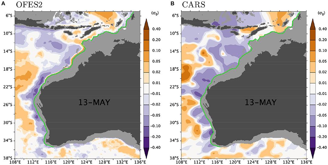
Figure 4. Potential density anomaly (A) for OFES2 and (B) for CARS Aus8 at 270 m on May 13. This depth is chosen because the density anomaly associated with the northeastward undercurrent is largest (Figure 5B). The green curve approximately follows the 200-m isobath (section 2.2.2).

3.2. Vertical Structure

Figure 5 shows the anomaly of v^r across the 13°S^r (15.6°S) and 19°S^r (19.9°S) sections (see the schematic map, Figure 1, for the “rotated latitude”). The northeastward-flowing undercurrent is located below the shelf break within the pycnocline and hugs the continental slope. In the 19°S^r section, the surface southwestward flow (the Holloway Current) has a clear narrow core above the undercurrent. In contrast, the surface core is weak in the 13°S^r section and the Holloway Current is broad. Unlike the undercurrent, the Holloway Current is not trapped to the shelf break or to the continental slope (Figure 3A), sometimes moving on to the continental shelf and sometimes wandering offshore. Its width also varies. It is interesting that an eddy-resolving oceanic re-analysis, HYCOM (Cummings and Smedstad, 2013; Helber et al., 2013), shows a similar undercurrent at a similar timing (Supplementary Figure S4).

FIGURE 5

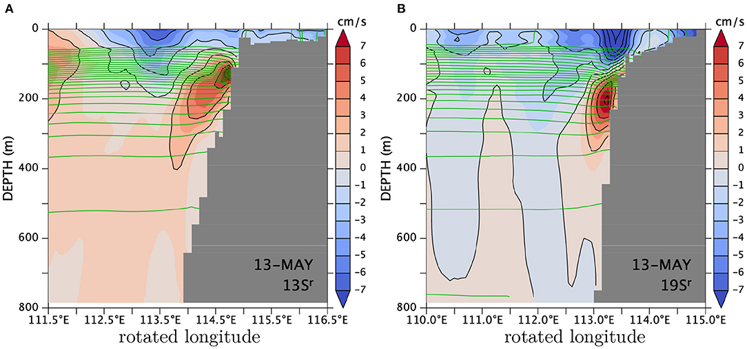
Figure 5. Annual anomaly of v^r (shaded) across the (A) 13°S^r (15.6°S) and (B) 19°S^r (19.9°S) sections on May 13. The green contours show potential density at an interval of 0.2σ_θ.

During February–March appears a negative (southwestward) undercurrent core (not shown) whose structure is similar to the positive core. This discussion has been on the annual anomaly field but in the raw velocity field, both the positive and negative undercurrent cores are clearly visible (not shown) as the annual mean velocity is weak here (see below).

The y-z structure of this undercurrent is depicted along the 200-m isobath in Figure 6. The positive anomaly of the “longshore” velocity appears to spread from ~1°S^r (7°S) counterclockwise along the continental slope down to at least 34°S (We will later discuss whether this is a continuous feature or not). South of 22°S, the vertical extent of the positive anomaly rapidly grows southward, and this depth range is comparable to that of the Leeuwin Undercurrent. In the North West Shelf region (north or northeast of 22°S), the undercurrent is shallower and its vertical extent is much smaller. Note the gradual deepening of the core of the undercurrent from, say, ~180 m at 10°S^r to ~210 m at 20°S^r.

FIGURE 6

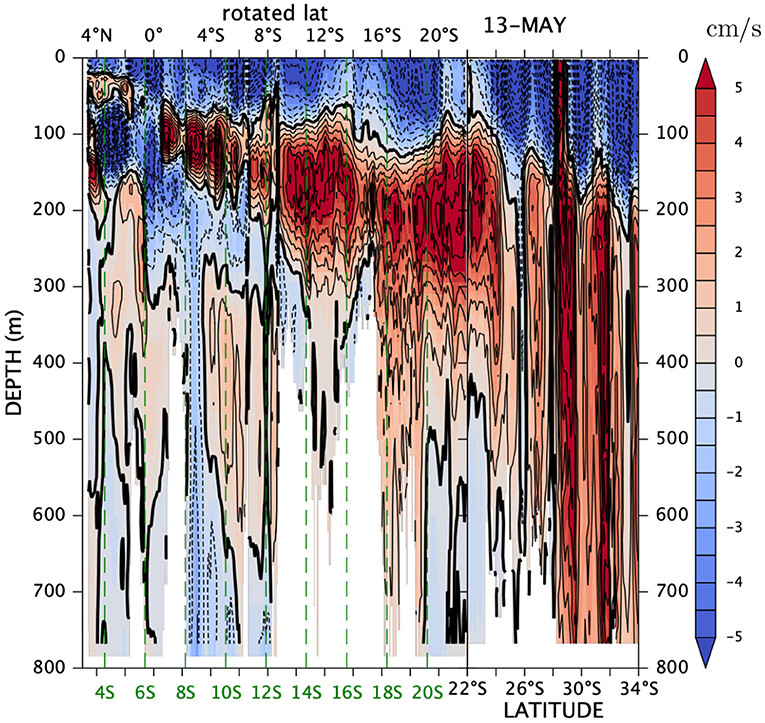
Figure 6. Annual anomaly along the shelf break on May 13 of longshore velocity averaged over the x_c strip, that is, between $x_{\mathrm{\text{c}}}-0.5^{°}$ and $x_{\mathrm{\text{c}}}+0.2^{°}$, where x_c(y) is the location of the 200-m isobath (see section 2.2.2). The North West Shelf region ( y > 22°S) and the west-coast region ( y < 22°S) are plotted on the left and right, respectively. Green numbers and green dashed vertical lines indicate true latitudes along the x^r = 0 axis and the black numbers above the plot are the rotated latitudes y^r. See the text and Figure 1.

A similar structure exists in the potential density anomaly from OFES2 (Supplementary Figures S2B,D). We have made comparable plots for the potential-density anomalies from CARS Aus8. These plots (Supplementary Figures S2A,C), however, do not show similar structures to OFES2's although the overall larger-scale structure is roughly similar. This result is consistent with the lack of density anomaly in the map for CARS Aus8 (Figure 4B).

3.3. Temporal Structure

If one looks at the animation (not shown) of Figure 6 over the climatological year, one notices that the phase lines generally migrate upward and southwestward below the shelf break (100–150 m) along the northwest coast. Figure 7 shows Hovmöller diagrams at a fixed rotated latitude and at a fixed depth. Below the shelf-break depth (~150 m; see Figure 5B), phases propagate upwards from 300 to 150 m in both velocity and density fields. In density there appears to be downward phase propagation above the shelf break, but this is probably a false impression due to the winter deepening and summer shoaling of the mixed layer (See Figure 5 for the mixed layer depth during May). At 160 m phase propagation is southward (Figures 7C,D). Its speed is roughly 0.2m/s, which is indicated by the green line. As discussed later, the region of southward and upward phase propagation deepens southward, reminiscent of the downward-southward slope in Figure 6.

FIGURE 7

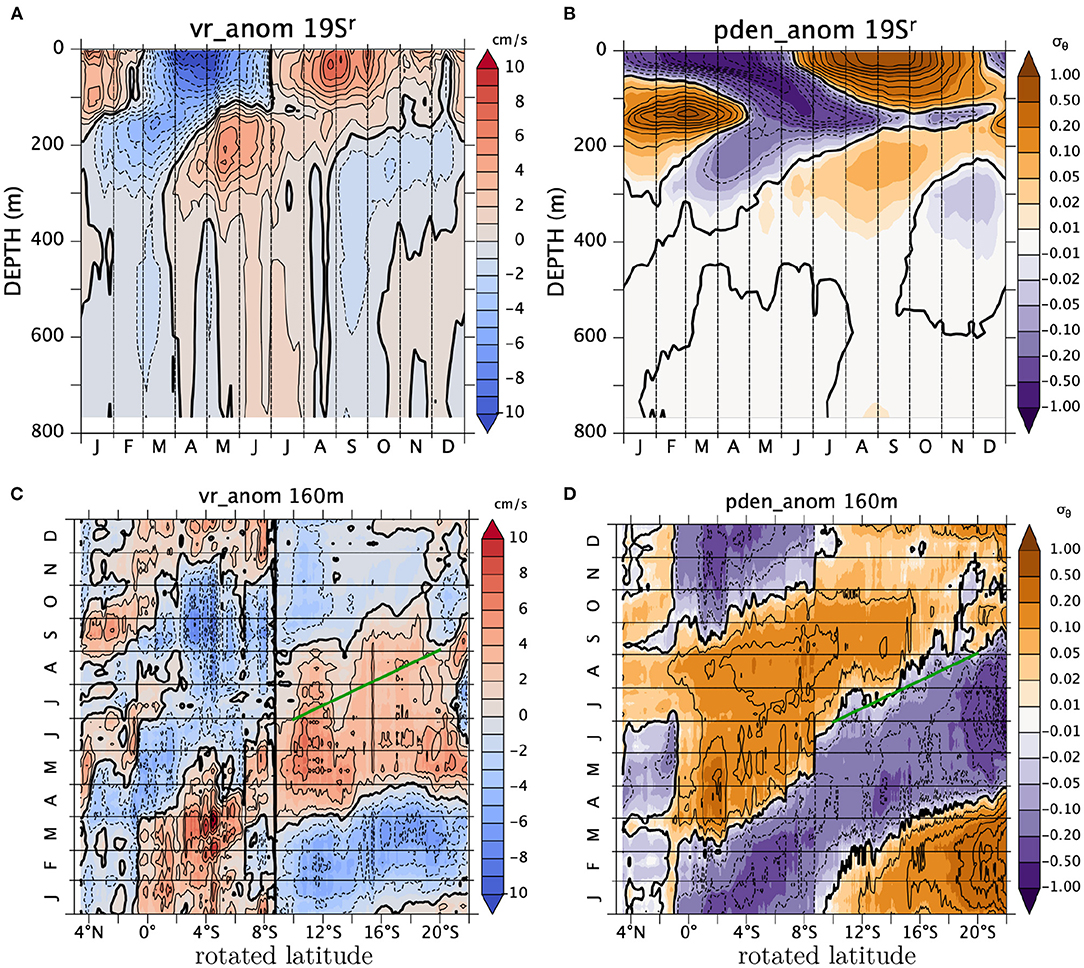
Figure 7. Depth–time Hovmöller diagrams of (A) longshore-velocity anomaly and (B) potential density anomaly at y^r = 19°S^r. Latitude–time Hovmöller diagrams of (C) longshore velocity anomaly and (D) potential density anomaly at z = −160 m. All quantities are averaged between $x_{\mathrm{\text{c}}}-0.5^{°}$ and $x_{\mathrm{\text{c}}}+0.2^{°}$, where x_c(y) is the location of the 200-m isobath. The green straight line indicates the southwestward propagation speed of 0.2m/s. Note that color intervals are uneven for density as the near-surface density anomaly is much larger than that associated with the undercurrent.

3.4. Fourier Components

Figure 8 shows the spectrum of longshore velocity over the region where the seasonal undercurrent is strong on the continental slope along the northwest coast. The annual signal is the strongest followed by the 1/2-annual (semi-annual) and the 1/3-annual. The mean flow, which is negative (southwestward, not shown), is less than 1 cm/s. In what follows, we focus on Fourier modes n = 1, 2, 3.

FIGURE 8

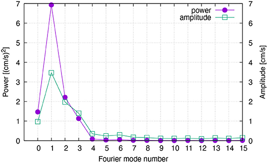
Figure 8. Power and amplitude spectra of longshore velocity averaged over the x_c strip (see section 2.2.2), 10°S^r–20°S^r, and 150–200 m. This region roughly coincides with the region where the seasonal undercurrent is strong (Figure 6). The amplitude of mode 0 is the absolute value of the temporal average, the latter of which is negative (not shown). The maximum Fourier mode number is 36 because there are 73 pentads in the 5-day climatology, but only the modes up to 15 is plotted. The remaining modes (not shown) are as weak as modes 4–15. The definitions of the spectra are standard but see section S1.2 in Supplementary Material S2, for the precise definitions.

Figure 9 shows the amplitude of longshore velocity for the n = 1–3 modes. South of 9°S^r (12.8°S) and below the surface maximum, there is a band of high amplitude that corresponds to the seasonal undercurrent shown in Figure 6. The amplitudes of higher harmonics are generally smaller and the cores shift to shallower depths south of 9°S^r. The phase field for the annual mode (Figure 9D) shows relatively smooth upward and southwestward propagation south of 9°S^r. At ~300 m, phase θ~0 (indicated by a thick contour line) and θ increases upwward past 90° (thin solid line) and then past 180° (thick line), which is the same as −180°, and keeps increasing from −180° past −90° (thin dashed line). In contrast, there is a sharp jump in phase across 9°S^r. The other two modes show a similar vertical propagation south of 9°S^r.

FIGURE 9

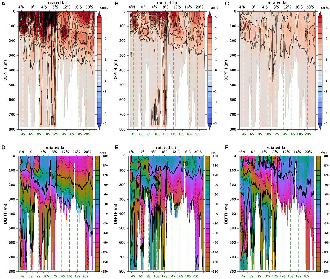
Figure 9. Amplitudes (A–C) and phases (D–F) of Fourier modes (A,D) n = 1 (annual) and (B,E) n = 2 (1/2-annual), and (D,F) n = 3 (1/3-annual) of longshore velocity. The phase angle uses the “phase” colormap in the cmocean collection (Thyng et al., 2016); the colormap is designed to be circular in such a way that −180° and 180° use an identical color. To guide the eye, thick contours are added at 0° and ±180°, thin solid contours at 90°, and thin dashed contours at −90°. The amplitude is averaged over the x_c strip whereas the phase is a slice at $x_{\mathrm{\text{c}}}(y^{\mathrm{\text{r}}})-0.35^{°}$. Phase values inevitably include artificial jumps, in the above case, across ±180°; an average of positive and negative values close to ±180° results in a value close to zero, which is totally wrong as an average of phase. For this reason we avoid averaging phase. The location of the slice is chosen so that the slice reaches at least 300 m at most places and at the same time avoids offshore shallow sea mounts (not shown) as much as possible.

This propagation is further visualized using Hovmöller diagrams (Figure 10). The vertical propagation (Figures 10A–C) in the undercurrent range (below ~150 m) is clear. The annual component propagates slower than the other two modes. The nodal depth (where the variability is minimal) shifts somewhat upwards for higher frequencies. Above the nodal depth, the propagation is still upwards for the annual mode, whereas it is downward for the 1/2-annual, and it is not clear for the 1/3-annual.

FIGURE 10

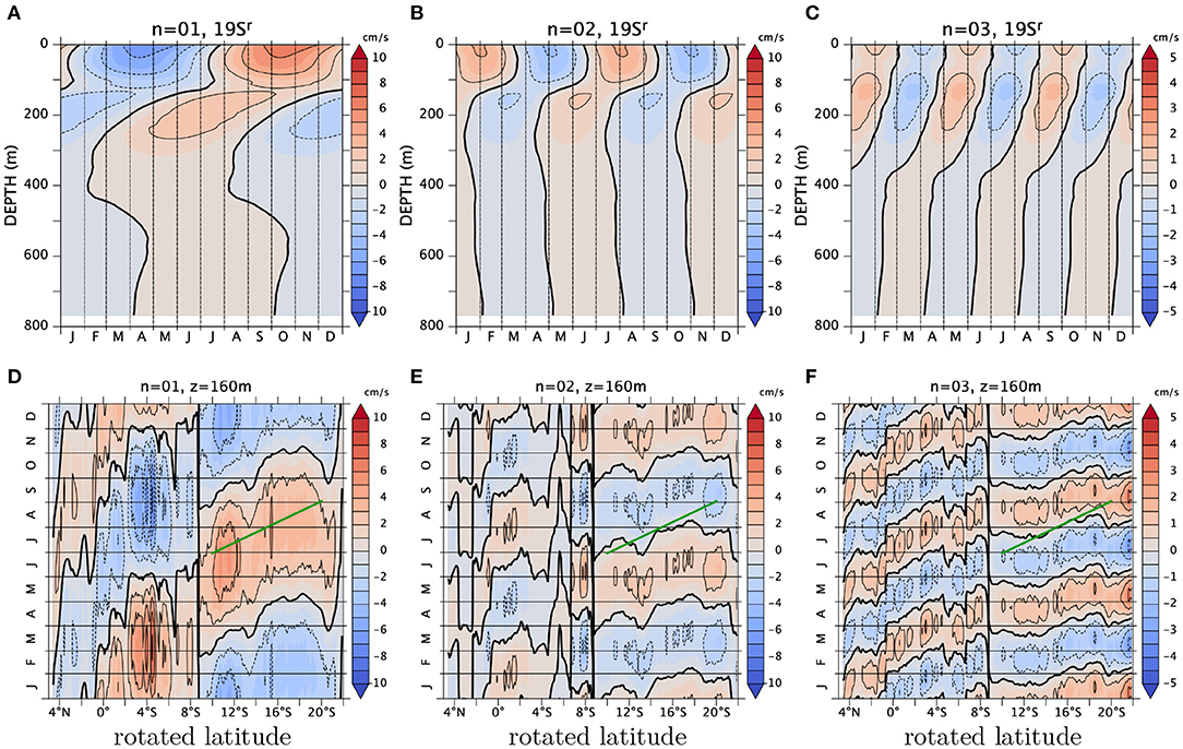
Figure 10. (A–C) z-t Hovmöller diagrams at 19°S^r and (D–F) y-t Hovmöller diagrams at 160 m for the annual (A,D), the 1/2-annual (B,E), and the 1/3-annual (C,F) harmonics of longshore velocity averaged over the x_c strip. The green lines indicate a phase speed of c_y = −0.2m/s.

The annual component shows a southwestward propagation (Figure 10D) at a speed of about −0.2m/s from 9°S^r to 20°S^r. The speed again appears to be smaller than those of the other two modes (Figures 10E,F) although the propagation speeds and directions are somewhat less regular for the higher modes than for the annual.

These three Fourier modes add up to create the (northeastward-flowing) undercurrent during April–May in the total field (Figure 7C). The negative phase (blue) in the annual harmonic during October–March (Figure 10D) is canceled during December–January and reinforced during February–March by the positive phases of the other two modes (Figures 10E,F). This is how the negative peak in the total field (Figure 7C) is constructed. This conclusion is supported by the fact that the actual superposition of the three Fourier modes (Supplementary Figure S5A) is almost indistinguishable from the original field (Figure 7C) southwest of 9°S^r.

Figure 11 shows the y-z structure of the three harmonics when the positive signal is strongest (Figure 6). The vertical extent of the undercurrent of each harmonic somewhat increases southwestward. In addition to that, the core of the undercurrent for higher modes is located at shallower depths. Both trends contribute to the vertical spreading of the positive anomaly in the total field (Figure 6). This conclusion is supported by the fact that the superposition of the three modes (Supplementary Figure S6A) is very similar to the original field southwest of 9°S^r (Figure 6 and Supplementary Figure S6B). Even though the phase discontinuity at 9°S^r (12.8°S) is not very clear in the total field, it is clearer in each Fourier mode (Figure 11). It is interesting that the contribution from higher Fourier modes is significant northeast of 9°S^r, that is, the difference between the superposition of the lowest three modes and the original field is significant northeast of 9°S^r (Supplementary Figure S6).

FIGURE 11

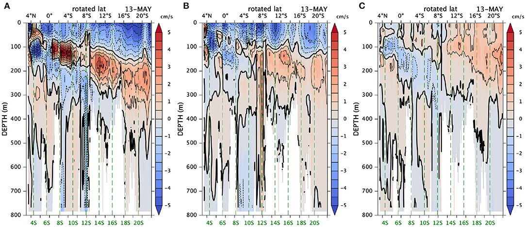
Figure 11. Same as Figure 6 but for the (A) annual, (B) 1/2-annual, and (C) 1/3-annual harmonics (n = 1, 2, 3).

3.5. Similarity to Coastal Trapped Waves

The southward and upward propagation of phase is reminiscent of coastal Kelvin waves (e.g., Romea and Allen, 1983). The x-z structure of the flow (Figure 5), however, suggests that the signal we have seen is a coastal trapped wave (CTW; e.g., Clarke, 1977; Brink, 1982b; Church et al., 1986a). At the frequencies we are interested in, however, our latitude range (5°S–22°S) of interest is well equatorward of the critical latitudes if c < 1.5m/s and c < 2.9m/s for the annual and semi-annual frequencies, respectively, for a 45° slanted coast line (see Introduction). It is not clear, however, whether CTWs completely propagate away as planetary Rossby waves (see Introduction). We here show an inviscid solution to a CTW model on an f plane in the hope that such a solution at least qualitatively captures some aspects of the true solution. The solution is outlined in section 2.3 and and details are provided in Appendix A. The appendix also discusses some salient properties of the solution which are not directly relevant to this comparison with the OGCM.

A periodic zonally-uniform meridional wind forces the ocean in the region 0 < y < L at the annual frequency. We set L= 500 km without any particular reason; this arbitrariness, however, does not affect our discussion because as Appendix Equation (A.3) indicates, the amplitude of the solution south of y is proportional to L but that is the only dependency on L. The solution takes the form of a “beam,” that is, the variability is limited to a narrow band which extends from the forcing region (Figure 12A). The amplitude of the wind stress is 0.1Pa (1 dyn/cm^2), to which velocity is proportional. The amplitude of the solution (larger than 30 cm/s; Figure 12A) is obviously much larger than that of the undercurrent in OFES2.

FIGURE 12

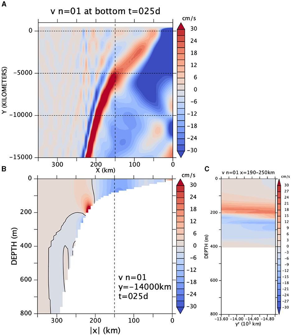
Figure 12. v from the CTW model (A) along the bottom, (B) at y = −14,000 km, and (C) averaged over x = 190–250 km at an arbitrary time for the annual frequency. The y-range for (C) is the southern-most 1,400 km of (A).

As high-order CTW modes are bottom trapped (Figure A2 in Appendix), the CTW beam is clearest along the bottom (Figure 12A). The beam propagates southward and gradually migrates down the slope and eventually emerges on to the continental slope to form an “undercurrent” (Figure 12B). An obvious problem is that the beam emerges on the continental slope only around y ~ −10,000 km, very far downstream (southward) from the forcing region (y > 0). This result suggests that the actual undercurrent in OFES2 is forced very near the continental slope, likely at the offshore protrusion at around 13°S (9°S^r) of the shelf break, where the shelf break rapidly changes its direction (Figure 1) and where the clear discontinuity occurs in phase (Figure 9).

Note that the idealized solution is constructed as a superposition of the lowest 24 modes (section 2.3 and Appendix A). This is not quite sufficient for this beam in that the summation is not well converged, and as a result, ripples remain outside the beam (Figure 12A) and the vertical propagation does not appear smooth (Figure 12C).

Figure 12B shows a crossshore section at y = −14,000 km where the “undercurrent” is seen between 100 and 200 m. There is a weaker counterflow further down the slope. This section is chosen so that the “undercurrent” comes down to a depth range similar to that of the undercurrent in Figure 5. Although the counterflow (blue) below the undercurrent is not visible in the total v^r field in Figure 5, it is visible in the annual harmonic from OFES2 (Figure 11). The 9°S^r–21°S^r portion of this latter OFES2 plot qualitatively resembles the y-z structure of the idealized model flow (Figure 12C), in that the beam gradually descends the slope. The descent is very slow at a few tens of meters over the y range of 1,400 km. The angle of descent is deeper for the annual harmonic velocity core in OFES2 (Figure 11A): 180 m at 10°S^r to 230 m at 20°S^r, the horizontal distance corresponding to about 1,100 km.

The Hovmöller diagrams Figure 13 are qualitatively similar to those from the model (Figure 7); the phase speed is somewhat faster (~0.3m/s) in the CTW solution than in OFES2 (Figures 7, 10D).

FIGURE 13

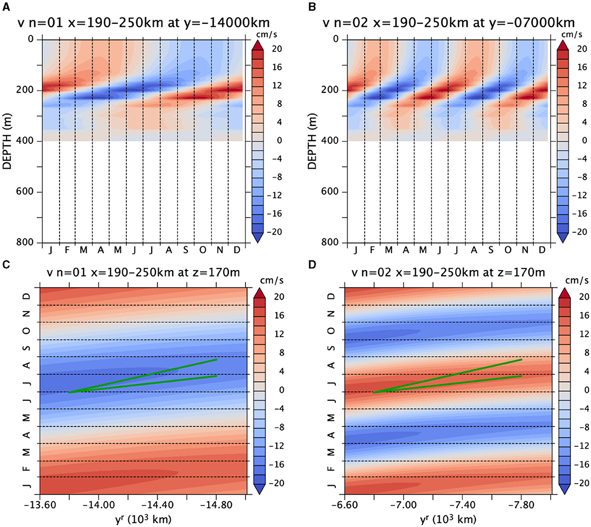
Figure 13. v from the CTW model averaged over x = 190–250 m (A) at y = −14,000 km and (B) at y = −7,000 km; and (C,D) at z = −170 m (A,C) for the annual frequency and (B,D) for the semi-annual frequency. The green line segments indicate speeds of 0.2m/s and 0.4m/s. Note that the latitudinal ranges are different between the annual (A,C) and semi-annual (B,D) frequencies because the beam emerges to the continental slope earlier for the semi-annual frequency. Note also that the range of coloring is narrower (±20 cm/s) here than in Figure 12 because the zonal average weakens the values.

The upward phase propagation is slower for the annual (Figure 13A) than for the semi-annual frequency (Figure 13B), consistent with the OGCM result (Figure 7). The difference in the meridional phase propagation (Figures 13C,D) is not very clear.

Some of the discrepancies may be due to the lack of dissipation in the present CTW model. This point will be taken up in section 4.3 below.

4. Summary and Discussion

A 5-day climatology is constructed from the output of an eddy-resolving oceanic general circulation model (OGCM) for the north and northwest regions of Australia. A seasonal northeastward-flowing undercurrent is found on the upper continental slope of the North West Shelf region during the climatological April–May (Figures 3B, 4A, 5, 6). An undercurrent with the opposite sign (southwestward) appears during February–March whose spatial structure is similar to that of the positive undercurrent. During its annual cycle, the phase of the undercurrent tends to propagate southwestward and upward (Figure 7).

The annual frequency dominates followed by the semi-annual and 1/3-annual frequencies (Figure 8), resulting in the northeastward peak during April–May and the southwestward peak during February–March (Figures 7C, 10D–F). The three Fourier components share the property that the phase tends to propagate southwestward and upward (Figures 9D–F, 10). The vertical structure of the current is predominantly that of the annual frequency (Figures 6, 11A) while the other two components contribute to spread the undercurrent upward (Figures 11B,C).

We then construct an idealized coastal trapped wave (CTW) solution driven by an idealized harmonic meridional winds at the annual and semi-annual frequencies. The solution takes the form of a beam originating from the forcing region at the coast and propagating offshore and southward (Figure 12A). When it emerges on to the continental slope, it takes the form of an undercurrent (Figure 12B). Like the OGCM counterpart (Figure 6), the undercurrent in the CTW model gradually deepens southwestward (Figure 12C). The upward and southward phase propagation of the undercurrent (Figure 13) is qualitatively consistent with that in the OGCM.

These pieces of evidence, however, are hardly sufficient to claim that the hypothesis—that the undercurrent is a beam of CTW—is proven. As discussed below, there are a number of discrepancies between the idealized model and the OGCM. Moreover, other mechanisms such as topographic rectification of fast variabilities (like tides) into slower variability or mean current (e.g., Brink, 2011) may also generate an undercurrent like the one we have found. We hope that the present study will inspire further exploration into the dynamics of the current in the future.

4.1. Critique of the Idealized CTW Model

In the idealized CTW model, the wind-forced beam emerges on to the continental slope far further downstream from the wind forcing (Figure 12B). This distance (~10,000 km) is totally unrealistic. If there were a place where the continental shelf is very narrow, the response could reach the continental slope sooner but the shelf is wide throughout the upstream region (Figure 1). This suggests that the beam is not directly generated by winds. See below.

Another interesting discrepancy between the CTW model and the OGCM is that the structure of the flow above the shelf-break depth is not consistent between the CTW model and OGCM. In particular the annual cycle of density anomaly above the shelf-break depth (Figure 7B) is not explained by the beam. The near-surface density structure is strongly affected by the winter cooling and summer warming and may not be strongly controlled by CTW dynamics.

As shown in Figure 3A, the surface current (Holloway Current) does not necessarily follow the shelf break, but when it does, it appears to form a “baroclinic pair” with the undercurrent (Figure 5), with a narrow surface current flowing in the opposite direction accompanying the undercurrent. The idealized beam solution does not have this property. This interesting feature may be due to a subsurface generation of CTW beams, as discussed in the next subsection.

Samelson's (2017) solution is appealing in that it produces both the undercurrent and the surface counterflow. For our case, the latter would be (a branch of) the Holloway Current. We are not sure what makes this difference between Samelson (2017) and the CTW model here. Samelson (2017) uses an inviscid, unstratified, f-plane, long-wave solution of coastal trapped waves on the continental shelf (the region where the bottom is shallower than 150 m), uses the solution as an eastern boundary condition for the stratified, β-plane quasi-geostrophic model on the continental slope, and obtains a steady solution to a zonally-uniform wind patch that exists only within a limited latitude band. The problem he solves is almost the same as we do, except that he considers the steady state, includes the β effect west of the shelf, and ignores stratification on the shelf. He also makes a different set of approximations. Some of these differences must be the cause. We leave this issue for a future study.

4.2. Generation

The undercurrent signal appears to originate from 13°S (9°S^r), as suggested by the discontinuity in phase (Figure 9). We have examined (not shown) the climatological (1991–2017) wind stress during May from J-OFURO3 version 1.1 (Tomita et al., 2019)³ but did not find any particular features there. As the 200-m isobath shows (Figure 1), the shelf break protrudes offshore and creates a feature like a submarine ridge at around 13°S (9°S^r). This sudden change in the topography is likely the cause of the discontinuity in phase.

It is possible that the wave is generated further northeast and keeps propagating along the shelf break across the submarine protrusion and the discontinuity in phase may be an artifact of the way we calculate the “zonal” (in x^r) average along $x_{\mathrm{\text{c}}}(y^{\mathrm{\text{r}}})$ (red line in Figure 1). Because following the actual 200-m isobath would not yield a single-valued function $x_{\mathrm{\text{c}}}(y^{\mathrm{\text{r}}})$, we simply connect the two end points of the part of the isobath extending in the northwestward direction. If we followed the actual 200-m isobath in some way, the discontinuity might disappear.

On the other hand, it is also possible that some coastal-trapped wave (CTW) originating from further northeast morphs into the high-order-mode CTW we have been examining. One potential mechanism is that of Dhage (2019). He explored how a submarine ridge protruding offshore from the continental slope scatters an incoming Kelvin wave or CTW into two beams, one propagating upward and the other downward from the top of the ridge. The downward propagating beam would fit the description of the beam in section 3. If this is really the case, the phase discontinuity at 13°S indicates the actual site of generation of the beam.

But, do we then see the upward-propagating beam above the depth of the shelf-break (top of the protrusion)? This is an interesting question. The upward beam would soon encounter the mixed layer and then it is not clear what happens to it. This process might be the cause of the surface counter flow associated with the undercurrent (Figure 5).

The generation of the current would be an interesting and important subject for future studies. In particular, this study has not explored potential link between the undercurrent and the variability upstream (northeast) of the submarine ridge at 13°S. Calculation of energy flux (Clarke, 1987) from OGCM data, for example, may be a good first step toward solving the problem.

4.3. Resolution and Friction

Figure 5 suggests that the undercurrent we have been examining is moderately well resolved by the model grid (1/10°). High-order CTW modes, however, should not be well resolved because of their small cross-shore scales (Figure A2).

Bottom friction or lateral viscosity or both is probably helping the OGCM to dissipate high-order CTWs. The bottom drag coefficient the OGCM uses (2.5 × 10⁻³) is comparable with the value in the CTWs by Brink (1982a) (although our OGCM does not prescribe RMS velocity to include unresolved high-frequency near-bottom flow). The continental slope is also a lateral boundary in OGCM so that the model's horizontal viscosity and diffusion (which are biharmonic) may also contribute to the dissipation.

Without dissipation, the idealized CTW beam remains narrow (Figure 12C). The downstream spread of the beam in OFES2 (Figure 6) may be due to the damping of high-order CTWs by friction. To test this idea, we modify the idealized CTW model to include an ad-hoc dissipation which is larger for higher-order modes, inspired by the formulation of internal vertical mixing in a similar model but with a flat bottom of McCreary (1981a) (Appendix A.3). With this modification, the beam spreads vertically (Supplementary Figure S7), with the bottom of the undercurrent deepening from 200 m at y = −13,600 km to 300 m at y = −15,000 km, this deepening comparable to that of the undercurrent in the OGCM between 9°S^r and 22°S^r (Figures 6, 11A).

For more quantitative analyses, bottom friction and other dissipation must be treated more carefully. If higher-order modes significantly contribute to the flow in reality, OGCMs would need more horizontal and vertical resolution to resolve the higher-order modes and the bottom boundary layer would need to be more carefully modeled in order to produce a quantitatively realistic undercurrent. If, on the other hand, high-order modes are quickly damped by dissipation, current resolutions of ~0.1° may be sufficient.

4.4. Leeuwin Undercurrent

It is not clear weather the undercurrent continues around the northwest corner (22°S) of Australia on to the west coast. Although it is very noisy, Figure 6 suggests that the vertical extent of the anomaly is much larger south of 22°S, where the Leeuwin Undercurrent (LUC) extends from 200 to 800 m (Furue et al., 2017). In contrast, the undercurrent along the North West Shelf is shallower and its vertical extent is much smaller (Figure 5B). It is, therefore, possible that the variability of the LUC is independent of the undercurrent along the northwest coast.

The continental slope is particularly steep around 22°S (Figure 1) and the beam might dissipate away there or our OGCM may not be able to resolve it there. This issue needs further investigation.

4.5. Offshore Branch

Figure 3B shows a broader northeastward flow offshore (northwest) of the undercurrent we have been examining. This offshore branch has a larger transport (Figure 3B) because its vertical extent is much larger (not shown). If one looks at the annual cycle of Figure 3B as animation (not shown), one notices that this branch propagates not only southwestward but also offshore. A similar tendency of westward propagation of meridional flow can be seen along the west coast of Australia (not shown). This variability might be representing a low-order Kelvin-wave-like wave.

4.6. Concluding Remarks

In conclusion, this study has described a seasonal undercurrent in an OGCM and proposed the hypothesis that it is a beam of coastal-trapped waves. It poses a number of interesting questions.

As discussed above, this study has not explored potential link of the undercurrent to variability upstream (northeast) of the submarine ridge at 13°S, nor has it explored the undercurrent's potential link to the surface flow. These issues are interesting subjects of future study. Once these problems are solved, we will know whether this undercurrent is a unique feature in the North West Shelf region or a similar flow exists everywhere.

It would be also important to explore observational data. Is it possible to tease out this signal from existing observations? CARS Aus8 is a gridded product interpolating hydrographic profiles. Analyzing raw hydrographic data may reveal the undercurrent. If the impacts of the undercurrent on the surface flow is established, it may be possible to extract undercurrent-related signal from sea-level data and the relation of the undercurrent with the Holloway Current may become clear.

We have only examined a climatological annual cycle. An implicit assumption there is that the variability is phase-locked to the annual cycle. But, if the undercurrent is indeed explained as CTWs, forcing which is not locked to the annual cycle should also be capable of driving similar undercurrent-like variabilities. Marin and Feng (2019), for example, found a variability in the surface current in the same region that is phase-locked to MJO (Madden-Julian Oscillation; Madden and Julian, 1971, 1994) events. There might be an undercurrent associated with this flow. Such signals, if any, would have been averaged out from our climatology. Examining the raw time series, therefore, will be an interesting future extension.

Data Availability Statement

The raw data supporting the conclusions of this article will be made available by the authors, without undue reservation (The monthly mean data is publicly available from https://doi.org/10.17596/0002029).

Author Contributions

RF contributed to the conception and design of the study, performed the analysis, and wrote the manuscript.

Funding

This work was partially supported by the Japan Society for the Promotion of Science through Grant KAKENHI 16K05562.

Conflict of Interest

The author declares that the research was conducted in the absence of any commercial or financial relationships that could be construed as a potential conflict of interest.

Publisher's Note

All claims expressed in this article are solely those of the authors and do not necessarily represent those of their affiliated organizations, or those of the publisher, the editors and the reviewers. Any product that may be evaluated in this article, or claim that may be made by its manufacturer, is not guaranteed or endorsed by the publisher.

Acknowledgments

This project started out as analysis of the annual cycle of the Leeuwin Current System with Tian Tian and Helen Phillips. The results of the original project is summarized in Tian's honours thesis. The OFES2 dataset (Sasaki et al., 2020) is produced and provided by Hide Sasaki. The data homepage is https://doi.org/10.17596/0002029⁴. The OFES2 integration was conducted on the Earth Simulator with the support of JAMSTEC. Ken Brink helped me with running Brink and Chapman's (1987) code. The programs are available from, and updates to them are documented in, https://www.whoi.edu/cms/files/Fortran_30425.htm (2007; accessed 2021-11-30). Discussion with Laxmikant Dhage and Ted Durland inspired the discussion of the potential mechanism of wave generation (section 4.2). Interaction with Lei Han and Jay McCreary was helpful in thinking about how to present the results of the data analysis in the present paper. Additionally Jay McCreary has provided me with insights and knowledge about linear coastal waves and planetary Rossby waves. Discussion with Ken Brink, Allan Clarke, Katsuro Katsumata, Humio Mitsudera, and Yuki Tanaka (alphabetical order) was helpful. Reviewers' comments helped substantially improve this manuscript. CARS Aus8 is available from http://www.marine.csiro.au/atlas/ (accessed 2021-10-08). J-OFURO3 is available from https://j-ofuro.isee.nagoya-u.ac.jp/en/ (accessed 2021-10-08). GOFS 3.1, 41-layer HYCOM + NCODA Global 1/12° Reanalysis is available from https://www.hycom.org/dataserver/gofs-3pt1/reanalysis (accessed 2021-11-28) and from http://apdrc.soest.hawaii.edu/ (accessed 2021-11-23). The author wishes to acknowledge use of the PyFerret program for analysis and graphics in this paper. PyFerret is a product of NOAA's Pacific Marine Environmental Laboratory (Information is available at http://ferret.pmel.noaa.gov/Ferret/).

Supplementary Material

The Supplementary Material for this article can be found online at: https://www.frontiersin.org/articles/10.3389/fmars.2021.806659/full#supplementary-material

Footnotes

1. ^https://doi.org/10.17596/0002029. The server is temporarily out of service as of this writing. The service will resume in the near future.

2. ^http://www.marine.csiro.au/atlas/

3. ^https://j-ofuro.isee.nagoya-u.ac.jp/en/

4. ^The server is temporarily out of service as of this writing. The service will resume in the near future.

References

Bahmanpour, M. H., Pattiaratchi, C., Wijeratne, E. M. S., Steinberg, C., and D'Adamo, N. (2016). Multi-year observation of Holloway Current along the shelf edge of North Western Australia. J. Coast. Res. 75, 517–521. doi: 10.2112/SI75-104.1

CrossRef Full Text | Google Scholar

Benthuysen, J., Furue, R., McCreary, J. P., Bindoff, N. L., and Phillips, H. E. (2014). Dynamics of the leeuwin current: part 2. The role of mixing and advection in a buoyancy-driven eastern boundary current over a continental shelf. Dyn. Atmos. Oceans. 65, 39–63. doi: 10.1016/j.dynatmoce.2013.10.004

CrossRef Full Text | Google Scholar

Brink, K. H.. (1982a). A comparison of long coastal trapped wave theory with observations off Peru. J. Phys. Oceanogr. 12, 897–913. doi: 10.1175/1520-0485(1982)012<0897:ACOLCT>2.0.CO;2

CrossRef Full Text | Google Scholar

Brink, K. H.. (1982b). The effect of bottom friction on low-frequency coastal trapped Waves. J. Phys. Oceanogr., 12, 127–133. doi: 10.1175/1520-0485(1982)012<0127:TEOBFO>2.0.CO;2

CrossRef Full Text | Google Scholar

Brink, K. H.. (1989). Energy conservation in coastal-trapped wave calculations. J. Phys. Oceanogr. 19, 1011–1016. doi: 10.1175/1520-0485(1989)019<1011:ECICTW>2.0.CO;2

CrossRef Full Text | Google Scholar

Brink, K. H.. (1991). Coastal-trapped waves and wind-driven currents over the continental shelf. Annu. Rev. Fluid Mech. 23, 389–412. doi: 10.1146/annurev.fl.23.010191.002133

CrossRef Full Text | Google Scholar

Brink, K. H.. (2011). Topographic rectification in a stratified ocean. J. Mar. Res. 69, 483–499. doi: 10.1357/002224011799849354

CrossRef Full Text | Google Scholar

Brink, K. H., and Allen, J. S. (1978). On the effect of bottom friction on barotropic motion over the continental shelf. J. Phys. Oceanogr. 8, 919–922. doi: 10.1175/1520-0485(1978)008<0919:OTEOBF>2.0.CO;2

CrossRef Full Text | Google Scholar

Brink, K. H., Bahr, F., and Shearman, R. K. (2007). Alongshore currents and mesoscale variability near the shelf edge off northwestern Australia. J. Geophys. Res. Oceans 112:C05013. doi: 10.1029/2006JC003725

CrossRef Full Text | Google Scholar

Brink, K. H., and Chapman, D. C. (1987). Programs for computing properties of coastal-trapped waves and wind-driven motions over the continental shelf and slope. Technical Report WHOI-87-24, Woods Hole Oceanographic Institution. Available online at: https://www.whoi.edu/cms/files/Fortran_30425.htm

Google Scholar

Cessi, P., and Wolfe, C. L. (2013). Adiabatic eastern boundary currents. J. Phys. Oceanogr. 43, 1127–1149. doi: 10.1175/JPO-D-12-0211.1

CrossRef Full Text | Google Scholar

Chelton, D. B., deSzoeke, R. A., Schlax, M. G., El Naggar, K., and Siwertz, N. (1998). Geographical variability of the first baroclinic Rossby radius of deformation. J. Phys. Oceanogr. 28, 433–460. doi: 10.1175/1520-0485(1998)028<0433:GVOTFB>2.0.CO;2

CrossRef Full Text | Google Scholar

Church, J. A., Freeland, H. J., and Smith, R. L. (1986a). Coastal-trapped waves on the East Australian continental shelf part I: propagation of modes. J. Phys. Oceanogr. 16, 1929–1943. doi: 10.1175/1520-0485(1986)016<1929:CTWOTE>2.0.CO;2

CrossRef Full Text | Google Scholar

Church, J. A., White, N. J., Clarke, A. J., Freeland, H. J., and Smith, R. L. (1986b). Coastal-trapped waves on the East Australian continental shelf part II: Model verification. J. Phys. Oceanogr. 16, 1945–1957. doi: 10.1175/1520-0485(1986)016<1945:CTWOTE>2.0.CO;2

CrossRef Full Text | Google Scholar

Clarke, A. J.. (1977). Observational and numerical evidence for wind-forced coastal trapped long waves. J. Phys. Oceanogr. 7, 231–247. doi: 10.1175/1520-0485(1977)007<0231:OANEFW>2.0.CO;2

CrossRef Full Text | Google Scholar

Clarke, A. J.. (1987). Origin of the coastally trapped waves observed during the australian coastal experiment. J. Phys. Oceanogr. 17, 1847–1859. doi: 10.1175/1520-0485(1987)017<1847:OOTCTW>2.0.CO;2

CrossRef Full Text | Google Scholar

Clarke, A. J., and Brink, K. H. (1985). The response of stratified, frictional flow of shelf and slope waters to fluctuating large-scale, low-frequency wind forcing. J. Phys. Oceanogr. 15, 439–453. doi: 10.1175/1520-0485(1985)015<0439:TROSFF>2.0.CO;2

CrossRef Full Text | Google Scholar

Clarke, A. J., and Gorder, S. V. (1994). On ENSO coastal currents and sea levels. J. Phys. Oceanogr. 24, 661–680. doi: 10.1175/1520-0485(1994)024<0661:OECCAS>2.0.CO;2

CrossRef Full Text | Google Scholar

Clarke, A. J., and Shi, C. (1991). Critical frequencies at ocean boundaries. J. Geophys. Res. Oceans 96:10731–10738. doi: 10.1029/91JC00933

CrossRef Full Text | Google Scholar

Cummings, J. A., and Smedstad, O. M. (2013). “Variational data assimilation for the global ocean,” in Data Assimilation for Atmospheric, Oceanic and Hydrologic Applications (Vol. II), eds S. K. Park and L. Xu (Berlin; Heidelberg: Springer), 303–343.

Google Scholar

D'Adamo, N., Fandry, C., Buchan, S., and Domingues, C. (2009). Northern sources of the Leeuwin Current and the “Holloway Current” on the North West Shelf. J. R. Soc. West. Aust. 92, 53–66.

Google Scholar

Dhage, L.. (2019). Vertical Coastal Trapped Wave Propagation Produced by a Subsurface Ridge (Ph.D. thesis). Oregon State University.

Google Scholar

Dunn, J. R., and Ridgway, K. R. (2002). Mapping ocean properties in regions of complex topography. Deep Sea Res. I 49, 591–604. doi: 10.1016/S0967-0637(01)00069-3

CrossRef Full Text | Google Scholar

Duran, E. R.. (2015). An investigation of the Leeuwin Undercurrent source waters and pathways (Honours thesis). University of Tasmania.

Duran, E. R., Phillips, H. E., Furue, R., Spence, P., and Bindoff, N. L. (2020). Southern Australia Current System based on a gridded hydrography and a high-resolution model. Prog. Oceanogr. 181:102254. doi: 10.1016/j.pocean.2019.102254

CrossRef Full Text | Google Scholar

Early, J. J., Lelong, M. P., and Smith, K. S. (2020). Fast and accurate computation of vertical modes. J. Adv. Model. Earth Syst. 12:e2019MS001939. doi: 10.1029/2019MS001939

CrossRef Full Text | Google Scholar

Freeland, H. J., Boland, F. M., Church, J. A., Clarke, A. J., Forbes, A. M. G., Huyer, A., et al. (1986). The Australian coastal experiment: a search for coastal-trapped waves. J. Phys. Oceanogr. 16, 1230–1249. doi: 10.1175/1520-0485(1986)016<1230:TACEAS>2.0.CO;2

CrossRef Full Text | Google Scholar

Furue, R., Guerreiro, K., Phillips, H. E., McCreary, J. P., and Bindoff, N. L. (2017). On the leeuwin current system and its linkage to zonal flows in the south indian ocean as inferred from a gridded hydrography. J. Phys. Oceanogr. 47, 583–602. doi: 10.1175/JPO-D-16-0170.1

CrossRef Full Text | Google Scholar

Furue, R., McCreary, J. P., Benthuysen, J., Phillips, H. E., and Bindoff, N. L. (2013). Dynamics of the Leeuwin Current: Part 1. Coastal flows in an inviscid, variable-density, layer model. Dyn. Atmos. Oceans. 63, 24–59. doi: 10.1016/j.dynatmoce.2013.03.003

CrossRef Full Text | Google Scholar

Gill, A. E.. (1982). Atmosphere-Ocean Dynamics. San Diego, CA: Academic Press.

Godfrey, J. S., and Ridgway, K. R. (1985). The large-scale environment of the poleward-flowing Leeuwin Current, Western Australia: longshore steric height gradients, wind stresses and geostrophic flow. J. Phys. Oceanogr. 15, 481–495. doi: 10.1175/1520-0485(1985)015<0481:TLSEOT>2.0.CO;2

CrossRef Full Text | Google Scholar

Helber, R. W., Townsend, T. L., Barron, C. N., Dastugue, J. M., and Carnes, M. R. (2013). Validation Test Report for the Improved Synthetic Ocean Profile (ISOP) System, Part I: Synthetic Profile Methods and Algorithm. Technical report, Oceanography Division, Naval Research Laboratory (Stennis Detachment), Stennis Space Center, Mississippi.

Google Scholar

Hughes, C. W., Fukumori, I., Griffies, S. M., Huthnance, J. M., Minobe, S., Spence, P., et al. (2019). Sea level and the role of coastal trapped waves in mediating the influence of the open ocean on the coast. Surv. Geophys. 40, 1467–1492. doi: 10.1007/s10712-019-09535-x

CrossRef Full Text | Google Scholar

Large, W., and Yeager, S. (2004). Diurnal to decadal global forcing for ocean and sea-ice models: The data sets and flux climatologies. Technical report, UCAR/NCAR.

Google Scholar

Levitus, S., Boyer, T. P., García, H. E., Locarnini, R. A., Zweng, M. M., Mishonov, A. V., et al. (2015). World Ocean Atlas 2013 (NCEI Accession 0114815).

Madden, R. A., and Julian, P. R. (1971). Detection of a 40–50 Day Oscillation in the Zonal Wind in the Tropical Pacific. J. Atmospheric Sci. 28, 702–708. doi: 10.1175/1520-0469(1971)028<0702:DOADOI>2.0.CO;2

CrossRef Full Text | Google Scholar

Madden, R. A., and Julian, P. R. (1994). Observations of the 40–50-Day tropical oscillation–a review. Mon. Weather Rev. 122, 814–837. doi: 10.1175/1520-0493(1994)122<0814:OOTDTO>2.0.CO;2

CrossRef Full Text | Google Scholar

Maiwa, K., Masumoto, Y., and Yamagata, T. (2010). Characteristics of coastal trapped waves along the southern and eastern coasts of Australia. J. Oceanogr. 66, 243–258. doi: 10.1007/s10872-010-0022-z

CrossRef Full Text | Google Scholar

Marin, M., and Feng, M. (2019). Intra-annual variability of the North West Shelf of Australia and its impact on the Holloway Current: excitement and propagation of coastally trapped waves. Cont. Shelf Res. 186, 88–103. doi: 10.1016/j.csr.2019.08.001

CrossRef Full Text | Google Scholar

Masumoto, Y., Sasaki, H., Kagimoto, T., Komori, N., Ishida, A., Sasai, Y., et al. (2004). A fifty-year eddy-resolving simulation of the world ocean: Preliminary outcomes of OFES (OGCM for the Earth Simulator). J. Earth Simulator 1, 35–56. doi: 10.32131/jes.1.35

CrossRef Full Text | Google Scholar

McCreary, J. P.. (1981a). A linear stratified ocean model of the coastal undercurrent. Philos. Trans. R. Soc. Lond. A 302, 385–413. doi: 10.1098/rsta.1981.0176

CrossRef Full Text | Google Scholar

McCreary, J. P.. (1981b). A linear stratified ocean model of the equatorial undercurrent. Philos. Trans. R. Soc. Lond. A 298, 603–635. doi: 10.1098/rsta.1981.0002

CrossRef Full Text | Google Scholar

McCreary, J. P.. (1984). Equatorial beams. J. Mar. Res. 42, 395–430. doi: 10.1357/002224084788502792

CrossRef Full Text | Google Scholar

McDougall, T. J., and Barker, P. M. (2011). Getting Started With TEOS-10 and the Gibbs Seawater (GSW) Oceanographic Toolbox. Battery Point, TAS: Trevor J McDougall.

Google Scholar

Merrifield, M. A., and Middleton, J. H. (1994). The influence of strongly varying topography on coastal-trapped waves at the southern Great Barrier Reef. J. Geophys. Res. Oceans 99, 10193–10205. doi: 10.1029/94JC00361

CrossRef Full Text | Google Scholar

Miyama, T., McCreary, J. P., Sengupta, D., and Senan, R. (2006). Dynamics of biweekly oscillations in the equatorial Indian Ocean. J. Phys. Oceanogr. 36, 827–846. doi: 10.1175/JPO2897.1

CrossRef Full Text | Google Scholar

Nethery, D., and Shankar, D. (2007). Vertical propagation of baroclinic Kelvin waves along the west coast of India. J. Earth Syst. Sci. 116, 331–339. doi: 10.1007/s12040-007-0030-6

CrossRef Full Text | Google Scholar

Noh, Y., and Kim, H. J. (1999). Simulations of temperature and turbulence structure of the oceanic boundary layer with the improved near-surface process. J. Geophys. Res. Oceans 104, 15621–15634. doi: 10.1029/1999JC900068

CrossRef Full Text | Google Scholar

Pacanowski, R. C., and Griffies, S. M. (2000). MOM 3.0 Manual. Princeton, NJ: Geophys. Fluid Dyn. Lab., NOAA.

Google Scholar

Phillips, H. E., Tandon, A., Furue, R., Hood, R., Ummenhofer, C., Benthuysen, J., et al. (2021). Progress in understanding of Indian Ocean circulation, variability, air-sea exchange and impacts on biogeochemistry. Ocean Sci. Discuss. 17, 1677–1751. doi: 10.5194/os-17-1677-2021

CrossRef Full Text | Google Scholar

Ridgway, K. R., Dunn, J. R., and Wilkin, J. L. (2002). Ocean interpolation by four-dimensional weighted least squares–application to the waters around Australia. J. Atmospheric Ocean. Technol. 19, 1357–1375. doi: 10.1175/1520-0426(2002)019<1357:OIBFDW>2.0.CO;2

CrossRef Full Text | Google Scholar

Ridgway, K. R., and Godfrey, J. (2015). The source of the Leeuwin Current seasonality. J. Geophys. Res. 120, 6843–6864. doi: 10.1002/2015JC011049

PubMed Abstract | CrossRef Full Text | Google Scholar

Romea, R. D., and Allen, J. S. (1983). On vertically propagating coastal Kelvin waves at low latitudes. J. Phys. Oceanogr. 13, 1241–1254. doi: 10.1175/1520-0485(1983)013<1241:OVPCKW>2.0.CO;2

CrossRef Full Text | Google Scholar

Samelson, R. M.. (2017). Time-dependent linear theory for the generation of poleward undercurrents on eastern boundaries. J. Phys. Oceanogr. 47, 3037–3059. doi: 10.1175/JPO-D-17-0077.1

CrossRef Full Text | Google Scholar

Sasaki, H., Kida, S., Furue, R., Aiki, H., Komori, N., Masumoto, Y., et al. (2020). A global eddying hindcast ocean simulation with OFES2. Geosci. Model Dev. 13, 3319–3336. doi: 10.5194/gmd-13-3319-2020

CrossRef Full Text | Google Scholar

Schloesser, F.. (2014). A dynamical model for the leeuwin undercurrent. J. Phys. Oceanogr. 44, 1798–1810. doi: 10.1175/JPO-D-13-0226.1

CrossRef Full Text | Google Scholar

Smith, R. D., Maltrud, M. E., Bryan, F. O., and Hecht, M. W. (2000). Numerical simulation of the North Atlantic Ocean at 1/10°. J. Phys. Oceanogr. 30, 1532–1561. doi: 10.1175/1520-0485(2000)030<1532:NSOTNA>2.0.CO;2

CrossRef Full Text | Google Scholar

St. Laurent, L. C., Simmons, H. L., and Jayne, S. R. (2002). Estimates of tidally driven enhanced mixing in the deep ocean. Geophys. Res. Lett. 29:2106. doi: 10.1029/2002GL015633

CrossRef Full Text | Google Scholar

Thompson, R. O. R. Y.. (1984). Observations of the Leeuwin Current off Western Australia. J. Phys. Oceanogr. 14, 623–628. doi: 10.1175/1520-0485(1984)014<0623:OOTLCO>2.0.CO;2

PubMed Abstract | CrossRef Full Text | Google Scholar

Thompson, R. O. R. Y.. (1987). Continental-shelf-scale model of the Leeuwin Current. J. Mar. Res. 45, 813–827. doi: 10.1357/002224087788327190

CrossRef Full Text | Google Scholar

Thyng, K., Greene, C., Hetland, R., Zimmerle, H., and DiMarco, S. (2016). True colors of oceanography: guidelines for effective and accurate colormap selection. Oceanography 29, 9–13. doi: 10.5670/oceanog.2016.66

CrossRef Full Text | Google Scholar

Tomita, H., Hihara, T., Kako, S., Kubota, M., and Kutsuwada, K. (2019). An introduction to J-OFURO3, a third-generation Japanese ocean flux data set using remote-sensing observations. J. Oceanogr. 75, 171–194. doi: 10.1007/s10872-018-0493-x

CrossRef Full Text | Google Scholar

Tsujino, H., Urakawa, S., Nakano, H., Small, R. J., Kim, W. M., Yeager, S. G., et al. (2018). JRA-55 based surface dataset for driving ocean–sea-ice models (JRA55-do). Ocean Model. 130, 79–139. doi: 10.1016/j.ocemod.2018.07.002

CrossRef Full Text | Google Scholar

Wang, D.-P., and Mooers, C. N. K. (1976). Coastal-trapped waves in a continuously stratified ocean. J. Phys. Oceanogr. 6, 853–863. doi: 10.1175/1520-0485(1976)006<0853:CTWIAC>2.0.CO;2

CrossRef Full Text | Google Scholar

Whitham, G. B.. (1974). Linear and Nonlinear Waves. New York, NY: John Wiley & Sons.

Google Scholar

Appendix

A. Coastal Trapped Waves

In this appendix, we show an idealized, simple solution of a coastal-trapped-wave (CTW) beam, which is referred to in the main text. Before doing so, however, we show a corresponding Kelvin-wave solution because the latter solution is instructive in order to understand a few salient aspects of the CTW solution. The Kelvin-wave solution we present here is essentially the same as those of Nethery and Shankar (2007).

A.1. Kelvin-Wave and Coastal-Trapped-Wave Modes

Let us assume a horizontally-uniform background stratification, linearize the primitive equations around a state of no motion with that stratification, and ignore viscosity or diffusion. We also assume a constant Coriolis parameter. The set of equations sustain waves trapped to a lateral boundary. We further make the “long-wave” assumption (that the longshore scales are much larger than the crossshore scales, etc.; see Brink, 1982a for details). For simplicity, assume that the only forcing is a curl-free longshore wind.

Let x and y be the crossshore and longshore coordinates. Then, a wave solution takes the form of

$\begin{array}{ll}p=\sum F_j(x,z){\varphi }_j(y,t),& (\mathrm{A1})\end{array}$

where ϕ_j is the solution to

$\begin{array}{ll}\left[-(1/c_j){\partial }_t+{\partial }_y\right]{\varphi }_j=b_j{\tau }^y(y,t).& (\mathrm{A2})\end{array}$

The solution to the latter equation is a wave that is forced by bτ and propagates in the negative y direction at a speed of c_j > 0. The “coupling coefficient” b_j, determined by the shape of the “mode” F_j(x, y), represents how strongly the wind forces mode j. The “modes” F_j are the solutions to an eigenvalue problem and c_j are the corresponding eigenvalues.

When the eastern boundary is a vertical wall, the eigenvalue problem is separable in x and z and the modes take the form of

$\begin{array}{ll}{F}_j(x,z)={\text{e}}^{x/(-c_j/f)}{\psi }_j(z),& (\mathrm{A3})\end{array}$

where ψ_j(z), in turn, are the solutions to the eigenvalue problem

$\begin{array}{ll}{\partial }_z[({\partial }_z{\psi }_j)/N^2]+{\psi }_j/c_j^2=0,{\partial }_z{\psi }_j{|}_{z=0,-h}=0,& (\mathrm{A4})\end{array}$

and c_j are the corresponding eigenvalues (e.g., McCreary, 1981a; Gill, 1982). This eigenvalue problem depends only on the given background stratification and can be solved numerically. (Note that because f < 0 for our case, the above eigenfunction decays westward x < 0 from the eastern boundary x = 0.) Together with Equations (2), (3), and (4), summation (1) gives the complete solution of the Kelvin wave response to the given meridional winds.

When the coastal bottom topography is taken into account, the eigenvalue problem for F(x, z) is no longer separable and the two-dimensional partial differential equation has to be solved numerically (e.g., Brink, 1982a; Church et al., 1986a). See below. In this paper, we call waves with the vertical wall “Kelvin waves” and waves with a sloping bottom “coastal trapped waves” or “CTWs”.

A.2. Kelvin-Wave and CTW Beams

We consider a solution forced by a simple periodic wind confined to the region 0 < y < L, of the form

$\begin{array}{l}{\tau }^y(y,t)=\{\begin{array}{ll}{G}_{\text{o}}(sin\alpha y){\text{e}}^{\iota \omega t}& 0\le y\le L,\\ 0& \text{otherwise,}\end{array}\end{array}$

where α ≡ π/L.

We further assume that there is no other forcing and therefore ϕ = 0 at y = L. We further ignore transients (free waves) and retain only the forced part of the solution, which is

$\begin{array}{ll}{\varphi }_j(y,t)=\{\begin{array}{ll}\frac{-\alpha G_{\text{o}}}{{\alpha }^2-l^2}[-\iota (l_j/\alpha )sin\alpha y+cos\alpha y+{\text{e}}^{-\iota l_j(y-L)}]{\text{e}}^{\iota \omega t}& 0<y<L\\ \frac{-\alpha G_{\text{o}}}{{\alpha }^2-l_j^2}(1+{\text{e}}^{\iota l_{j}L}){\text{e}}^{\iota l_{j}y}{\text{e}}^{\iota \omega t}& y<0,\end{array}& (\mathrm{A5})\end{array}$

where l_j ≡ −ω/c_j < 0 is the longshore wavenumber. The negative sign of l_j indicates that the wave propagates in the negative y direction.

For the basic density stratification, we use the annual mean salinity and temperature fields from the World Ocean Atlas 2013 (Levitus et al., 2015) as the OFES2 data below 800 m has not been processed and is not easily accessed and because for this theoretical, idealized calculation, the precision of the background stratification should not matter much. We select the deep ocean that satisfies

$112^{°}<\text{lon}<120^{°},-20^{°}<\text{lat}<-12^{°},\text{lat}-\text{lon}\ge -134.5^{°}.$

The last condition is to exclude the shelf region. We first horizontally average salinity and temperature within the above region; we then calculate potential density referred to the sea surface and calculate the Brunt-Väisälä frequency (BVF) from potential density on WOA's vertical grid, using the Gibbs Sea Water Oceanographic Toolbox (McDougall and Barker, 2011); we then remove negative BVF values and finally interpolate onto a new grid which is uniform in the “stretched coordinate” (e.g., Early et al., 2020). The last treatment is necessary to avoid unphysical modal shapes at high-order modes.

A.2.1. Kelvin-Wave Beam

When the bottom is flat, we numerically solve Equation (4) for the vertical modes using the background stratification and the maximum depth is set to 5,000m. Figure A1 shows the top 300 m of a few lowest-order modes and the j = 100 mode. Note that the local vertical wavelength of each mode is smallest where N is largest and even there the 100th mode is well resolved.

FIGURE A1

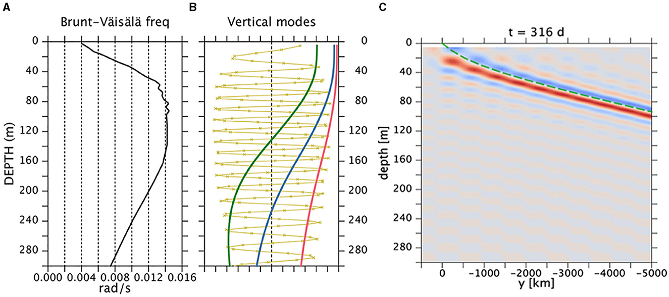
Figure A1. (A) Mean Brunt-Väisälä frequency N(z) based on WOA13 and (B) vertical modes 1, 2, 3, and 100 (red, blue, green, and yellow). The dots on the j = 100 mode indicate the gridpoints for the numerical calculation of Equation (4). (C) Meridional velocity (snapshot at an arbitrary time and at x = 0, eastern boundary) of coastal Kelvin wave on an f plane forced by an annual wind. The velocity field is constructed as a sum of 100 modes [ j = 1–100 in formula (1). The total depth is 5,000 m; only the upper 300 m is shown. The green dashed curve is a WKB ray starting from the southern edge of the forcing region (y > 0). See text for details.

The Kelvin-wave solution is then Equation (1) with Equation (3) and shown in Figure A1C. As is well-known (e.g., McCreary, 1984), the phase propagates upward and southward (not shown) and the wave solution takes the form of a “beam”, that is, the amplitude of the wave is large only in a narrow band. The beam extends from the forcing region (y > 0) at the surface downward and southward. The angle of the beam becomes deeper (steeper) as the frequency increases (not shown, but see Nethery and Shankar, 2007).

If the summation of the modes is extended to infinity, the variability is confined all within the narrow beam, but with only the 100 modes, weak stripes remain above and below the beam. The plot therefore indicates that even 100 modes are not quite sufficient.

The trajectory of the beam (“ray”) can be calculated as follows. A derivation of the ray equation is provided in McCreary (1984) for various equatorial waves. The following derivation is for the coastal Kelvin wave but is the same as McCreary's (1984) one for the equatorial Kelvin wave. We apply the WKB approximation to Equation (4); that is, we assume that ψ ∝ e^−ιmz, which gives

$\begin{array}{l}-(m^2/N^2)\psi +\psi /c^2=0\\ \Rightarrow c=N/\left|m\right|\end{array}$

and therefore the dispersion relation becomes ω = −lc = −Nl/|m|. The ray path is then

$\frac{\partial y}{\partial z}=\frac{\partial \omega /\partial l}{\partial \omega /\partial m}=-\frac{m}{l}=\frac{N}{\omega }sign(m)$

(e.g. Whitham, 1974). For a solution with upward-propagating phase (m > 0), the ray path slopes down southward (in the negative-y direction) according to

$\begin{array}{l}y(z)=y_o-\frac{1}{\omega }{\displaystyle {\int }_z^{z_o}}d{z}^{\prime }N(z^{\prime }).\end{array}$

The group velocity of the ray is downward and southward whereas the phase propagates upward and southward. This WKB ray is indicated by the green curve in Figure A1 with (y_o, z_o) = (0, 0).

A.2.2. Coastal Trapped Wave Beam

We carry out the same exercise for CTWs. The F(x, z) modes and corresponding wave speeds c are numerically calculated using Brink and Chapman's (1987) Fortran program, for the background stratification described above. The bottom profile is an average of OFES2's bottom profile in x^r over 19°S^r–12°S^r, where the bottom topography is relatively smooth but still varies considerably in the longshore (y^r) direction. Because of this averaging, the resultant profile does not have as clear a shelf break as the individual profiles (Figure 5). We finally weakly smooth the profile in the x direction using polynomial fitting (Figure A2) and truncate it at 2,000 m, which we set to be the maximum depth for the CTW mode calculation.

FIGURE A2

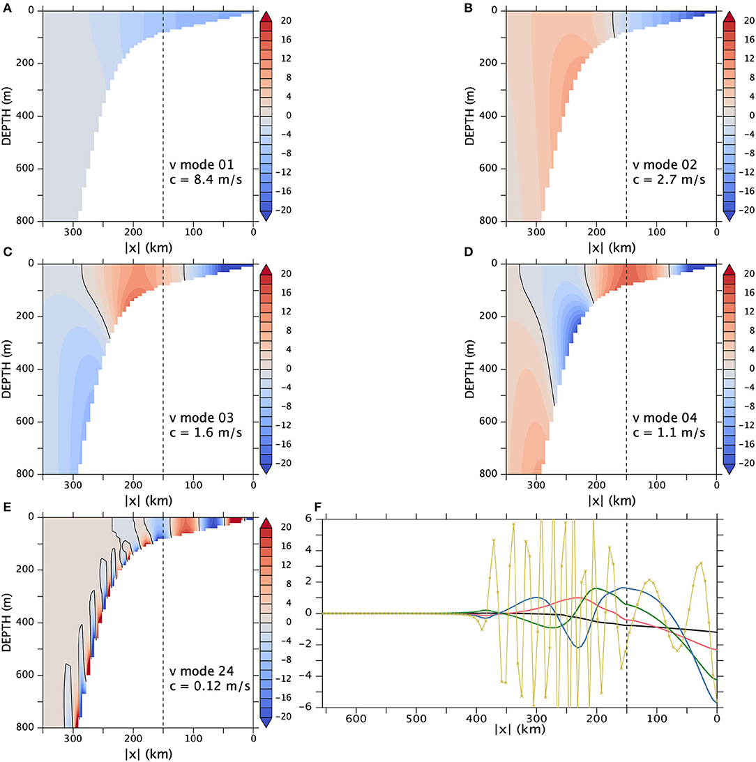
Figure A2. CTW modes j = 1–4 and 24 for v. (A–E) x-z structure; (F) x profiles along the bottom, where the gridpoints are marked for the j = 24 mode to show that the horizontal resolution is marginal for this mode. A dashed line is plotted at x = −150 km to roughly mark the transition from the continental shelf to the continental slope.

We have been able to obtain up to 24 modes, among which modes 1–4 and 24 are shown in Figure A2. We have confirmed that the number of zero-crossings is the same as the mode number of each mode (Brink and Chapman, 1987). This consideration, however, is still not sufficient. High-order modes have amplitudes trapped to the bottom slope, and the x profile of a mode along the bottom has short wavelengths where the bottom slope is steep (Figure A2). If the gridspacing in the x direction is not small enough to resolve these wavelengths at the steepest slope, the modes come out as totally unphysical profiles (not shown) even thought they have the right number of zero-crossings. We have examined all 24 modes to confirm that the wavelengths are resolved even at the steepest slope. We had to stop at 24 modes because the horizontal resolution is marginal at j = 24 on the continental slope (Figure A2). Beyond this mode, the eigenfunctions jump to unphysical profiles. We have also confirmed that the profiles of the modes only gradually change as the mode number increases.

We then sum up the wave response (A5) over the 24 modes as (A2) to obtain the total 4-dimensional (x, y, z, t) solution forced by the idealized wind patch. The v response is similarly obtained by replacing F_j's with the corresponding modes for v (Brink and Chapman, 1987).

As the Kelvin wave packet forms a beam in the y-z plane (Figure A1), the CTW solution forms a “beam”, but this time, the feature is most clear along the bottom in the x-y map (Figure 12A). This is because the higher-order CTW waves are trapped to the bottom (Figure A2). Twenty-four modes are not sufficient to obtain a clean beam: there are ripples down the continental slope (Figure 12A), where wave energy should not have reached.

As the spatial scales of the mode become closer to the grid spacing as for the j = 24 mode (Figure A2F), the numerical solution F_j and its eigenvalue c_j tend to become less accurate compared to the true (continuous) solution. Exact impacts of this problem will be clarified only when we reduce the grid spacing, but they are not likely critical for our problem because the main effect high-order modes have in the solution is to tighten the beam and the overall properties of the beam is determined by low-order modes. This hypothesis is supported by the solution with strong damping of high-order modes discussed in Appendix A3, where the largest impact of friction is to broaden the beam.

It is possible to construct a “fake” or “empirical” ray along the bottom. Let us consider a Sturm-Liouville eigenvalue problem analogous to Equation (4)

${\partial }_x[({\partial }_x{\psi }_j)/M]+{\psi }_j/c_j^2=0$

with suitable boundary conditions. We set M in such a way that M is positive and small on the continental shelf, M is positive and large on the continental slope, and M < 0 in the deep flat-bottom region. The local wavelength of ψ_j(x) is then large on the shelf and small on the slope; and ψ_j(x) exponentially decays in the flat-bottom region. In this way, we obtain a set of eigenfunctions that qualitatively resemble the x profiles of the actual modes along the bottom (Figure A2F) and corresponding eigenvalues c_j, which are in order-of-magnitude agreement with the actual eigenvalues of F_j. Using the same WKB approximation as used for the Kelvin waves, then, a ray path is obtained for a given frequency; this ray roughly follows the beam in Figure 12A.

A.3. Friction

McCreary (1981a) considered the same continuously-stratified linear model as we have been discussing in a flat-bottom ocean, where he included a parameterization of vertical mixing in the form of ν = κ = A/N², where A is an empirical constant and N is the background Brunt-Väisälä frequency. This parameterization leads to an additional linear-damping term of the form −r_ju_j, −r_jv_j, or −r_jp_j in the momentum or thickness equation for each vertical mode, where $r_j=A/c_j^2$. As a result, the y-t wave equation (A2) is modified to

$\begin{array}{ll}[-(1/c_j)({\partial }_t+r_j)+{\partial }_y]{\varphi }_j=b_j{\tau }^y(y,t)& (\mathrm{A6})\end{array}$

and the solution is identical to (A5) except that −ιl_j of (A5) is replaced with −ιl_j + (r_j/c_j) in the present solution. The solution decays in the negative y direction and the decay scale strongly depends on c_j with stronger damping associated with smaller c_j (i.e., larger mode number j).

For simplicity, we borrow this damping instead of solving again for CTW modes with bottom friction (Appendix A.4) even though McCreary (1981b) formalism is designed to represent internal diapycnal mixing, not bottom friction. We set A= 10-8 m²/s³ (which would give a vertical diffusivity of κ = A/N² ~ 10-4 m²/s in the main pycnocline, where N ~ 10-2 rad/s). The result is shown in Supplementary Figure S7: in this case, the beam spreads vertically, qualitatively similarly to the undercurrent in OFES2 (Figure 6) and the amplitude of the flow becomes much smaller.

A.4. Discussion

The original formalism and Brink and Chapman's (1987) code allow for bottom drag and variation in f in the crossshore direction, but we neglect these effects in the present paper. It is also possible to take into account slow longshore variations of model parameters, solve the eigenvalue problem for F and c at each y, solve (2) with the y-dependent c, and obtain the final solution (1) (Brink, 1989). For our simple calculation, however, we also ignore this possibility and use just one bottom profile z = −h(x) and one density stratification N(z).

If the background stratification has a sharp jump, as at the bottom of the surface mixed layer, the Kelvin-wave beam generated at the sea surface is partially reflected. [This property is shown for Yanai-wave beams in Miyama et al. (2006).] The sum of the modes (1) automatically produces this type of solution (Miyama et al., 2006). Figure A1 does not include such a reflection because the stratification is presumably smooth enough.

On the other hand, the CTW beam along the bottom seems to show this type of reflection: In Figure 12A, the blue region first extends southwest, is reflected back eastward around x= -100 km, hits the eastern boundary at y= -12,000 km, and is reflected back westward. This property is probably due to the rapid change in the bottom slope between x= -100 km and -200 km.

It is also interesting that the part of the beam that emerges onto the continental slope (red) is intensified at x= -150 km. As indicated in Figures 12B, A2, the WTC modes are bottom trapped on the continental slope whereas they are less so on the shelf. This property implies that the energy of the beam is spread over the water column on the shelf but is focused toward the bottom when the beam emerges on the continental slope. There must be, therefore, downward propagation of energy when the beam is on the shelf.