 Laurence V. Madden1*
 Peter S. Ojiambo2
- 1Department of Plant Pathology, The Ohio State University, Wooster, OH, United States
- 2Center for Integrated Fungal Research, Department of Entomology and Plant Pathology, North Carolina State University, Raleigh, NC, United States
Modern data analysis typically involves the fitting of a statistical model to data, which includes estimating the model parameters and their precision (standard errors) and testing hypotheses based on the parameter estimates. Linear mixed models (LMMs) fitted through likelihood methods have been the foundation for data analysis for well over a quarter of a century. These models allow the researcher to simultaneously consider fixed (e.g., treatment) and random (e.g., block and location) effects on the response variables and account for the correlation of observations, when it is assumed that the response variable has a normal distribution. Analysis of variance (ANOVA), which was developed about a century ago, can be considered a special case of the use of an LMM. A wide diversity of experimental and treatment designs, as well as correlations of the response variable, can be handled using these types of models. Many response variables are not normally distributed, of course, such as discrete variables that may or may not be expressed as a percentage (e.g., counts of insects or diseased plants) and continuous variables with asymmetrical distributions (e.g., survival time). As expansions of LMMs, generalized linear mixed models (GLMMs) can be used to analyze the data arising from several non-normal statistical distributions, including the discrete binomial, Poisson, and negative binomial, as well as the continuous gamma and beta. A GLMM allows the data analyst to better match the model to the data rather than to force the data to match a specific model. The increase in computer memory and processing speed, together with the development of user-friendly software and the progress in statistical theory and methodology, has made it practical for non-statisticians to use GLMMs since the late 2000s. The switch from LMMs to GLMMs is deceptive, however, as there are several major issues that must be thought about or judged when using a GLMM, which are mostly resolved for routine analyses with LMMs. These include the consideration of conditional versus marginal distributions and means, overdispersion (for discrete data), the model-fitting method [e.g., maximum likelihood (integral approximation), restricted pseudo-likelihood, and quasi-likelihood], and the choice of link function to relate the mean to the fixed and random effects. The issues are explained conceptually with different model formulations and subsequently with an example involving the percentage of diseased plants in a field study with wheat, as well as with simulated data, starting with a LMM and transitioning to a GLMM. A brief synopsis of the published GLMM-based analyses in the plant agricultural literature is presented to give readers a sense of the range of applications of this approach to data analysis.
1 Introduction
Whether one is conducting a planned experiment with replication, blocking, and randomization or collecting observational data such as from a survey, data analysis needs to be carried out in order to reach conclusions (Schabenberger and Pierce, 2002). We take it as axiomatic that appropriate statistical methods are required to interpret the collected data from any study. Of course, “appropriate” can mean many different things, depending on the situation and context of interest. Generalized linear mixed models (GLMMs) are becoming quite popular for data analysis in agriculture and other disciplines (Gbur et al., 2012; Ruíz et al., 2023); however, there is a lot of uncertainty about which GLMM to use, how to fit GLMMs to data, and how to interpret the obtained results. Our objectives here were to provide some background on the statistical modeling of data, particularly for data collected in the agricultural or the plant sciences, to explain GLMMs with examples, and to discuss several important issues when using GLMMs that may be initially not appreciated by the data analyst.
Several other references are valuable for learning more about GLMMs and for conducting analyses of a wide range of datasets from different experimental designs (Littell et al., 2006; Bolker et al., 2009; Zuur et al., 2009; Gbur et al., 2012; Stroup, 2013; Brown and Prescott, 2015; Stroup et al., 2018; Gianinetti, 2020; Li et al., 2023; Ruíz et al., 2015, 2023). For those who wish to learn more theory, as well as applications, Stroup (2013) is an indispensable reference. Molenberghs and Verbeke (2010) and McCulloch and Searle (2001) provided considerably more theory about mixed models, but may be of less value to the reader of this article. This article is heavily influenced by Stroup (2013, 2015) and the material in Chapters 11–13 in Stroup et al. (2018). We focus on an example involving the percentage of plants infected by a particular disease in a field study, although the methods can be applied to any discrete data where percentages can be calculated. Gianinetti (2020) and Li et al. (2023) are other excellent references for the GLMM-based analysis of data expressed as percentages. Readers should refer to Gbur et al. (2012); Stroup (2013), and Ruíz et al. (2023) for details on the analysis of continuous data using GLMMs. For those interested in broader issues related to statistical analysis in horticulture, including commonly made errors, we recommend Kramer et al. (2016).
Below, we start with some historical background on data analysis, followed by a discussion on non-normal statistical distributions and then presentations on models for data with normal and non-normal distributions. Model expansions and alternatives are given for select experimental designs. We place an emphasis on the different methods of model fitting and the interpretation of the estimated parameters for GLMMs, demonstrated with an example dataset. Some major challenges in the use of GLMMs are presented. Before the conclusions, a list of cases in the literature where GLMMs were used is given.
2 Background: from ANOVA to GLMMs
Analysis of variance (ANOVA), including the special case of t-tests, and linear regression have been the foundations for data analysis in agriculture and other disciplines for over a century (Fisher, 1918, 1935; Cochran and Cox, 1957; Steel and Torrie, 1960). The pioneering statistical works of Fisher, Yates, Cochran, and Snedecor, among others, coupled with the advances in statistical software and the increased speed and memory of computers, have given researchers a large toolbox of methods to describe data, predict outcomes, and make inferences about hypotheses of interest (Schabenberger and Pierce, 2002; Gbur et al., 2012).
ANOVA can be considered a special case of multiple linear regression (Speed, 2010), where several predictor or explanatory variables (X1, X2, etc.) are binary (0, 1). This allows data analysis to be couched in terms of linear modeling of the response variables as functions of predictor variables, an approach that still dominates today. An explanatory variable can be discrete, generally known as a classification or class variable, or simply a factor, and consists of two or more distinct levels (e.g., cultivar 1 and cultivar 2 or treatment A and treatment B). Otherwise, the explanatory variable can be continuous (e.g., temperature), often called a covariate or a covariable. Continuous variables can be treated as discrete variables in a statistical model, depending on the objective and the manner in which the experiment was conducted.
Models consist of fixed-effects and/or random-effects variables (Schabenberger and Pierce, 2002). For the fixed-effects variables, the levels (categories or groups) in the study represent all possible levels of the factor or all the levels of interest by the investigator (i.e., they were selected for study because they are of specific interest). Examples would be fungicide treatment, biocontrol treatment, pathogen inoculum dose, temperature, cultivar, or the nitrogen level in a fertilizer. For the random-effects variables, the levels in the study represent only a random sample of a larger set of levels (i.e., a sample from a distribution of effects). Examples could include the location (environment), a block, or a plot in a field study. A given variable could be considered fixed or random, depending on the circumstances. For instance, plant genotype could be considered a random-effects variable if a sample of a population of genotypes was randomly selected for study, with the goal of characterizing the mean (expected value) and the variability of the response variable (e.g., yield); on the other hand, genotype could be considered as a fixed-effects variable if the investigator was strictly interested in the responses of those particular genotypes. Similar arguments can be made about location–year (“environment”) as being fixed or random (see Chapter 6 in Littell et al., 2006).
The term mixed model is used when there are both fixed- and random-effects variables in the model. More specifically, these are known as linear mixed models (LMMs) when the response variable (e.g., yield, biomass, or disease severity) is considered to be normally distributed and the mean (expected value) is modeled directly as a function of the fixed- and random-effects terms (Stroup, 2013). This is explained in the next section, which includes a more technical description of LMMs. A special case of a LMM is the linear model (LM), in which there are no random effects except for the residual; another special case is the random-effects model, in which there are no fixed-effects variables. The concept of random effects goes back to Fisher (1918, 1935), possibly earlier (but less formally), with subsequent important early contributions by Yates (1940) and Eisenhart (1947), as well as many others.
For many years, the standard approach to handling random effects in standard software (or by brute force work on a calculator in the very early days) was to fit a LM to the data using ordinary least squares as if all effects were fixed and then perform post-model-fitting calculations to estimate the mean squares and variances for the random-effects variables (Steel and Torrie, 1960; Littell et al., 2006). The latter are used (automatically) to estimate the standard errors (SEs) of the least squares means and the mean differences for the fixed-effects terms and also to test for factor effects. This approach works fine for many special cases (e.g., balanced randomized complete block designs); however, even for a design such as the popular split plot or split plot with blocks, certain SEs cannot be calculated correctly (Littell et al., 2006). For incomplete block designs (i.e., where each block does not contain all the treatments), recovering all of the available information in a study (e.g., treatment effects within and between blocks) requires some tedious post-model-fitting calculations when all factors (including blocks) are considered fixed in the model (Yates, 1940). Many other situations often cannot be analyzed satisfactorily with the mean square, post-model-fitting adjustment approach, at least not without major approximations. Examples include repeated measures in time and space or any situation when complex correlations of data need to be specified or estimated.
The methodology of treating random effects fully as random in the model-fitting process was developed by Henderson in a series of papers (e.g., Henderson, 1950, 1953, 1984), with extensive theory by Harville (1977) and others, especially Laird and Ware (1982). The model-fitting approach is likelihood-based (rather than least squares/mean square-based), with an assumed normal distribution for the response variable conditional on the random effects (see below). Except for special (simple) cases, model fitting is iterative, facilitated by fast computers with large memories to carry out the multiple iterations in a rapid manner. It was not until the mid-1990s that (relatively) easy-to-use software was developed to fit LMMs to data based on the likelihood principle. The MIXED procedure in SAS is especially important here (Littell et al., 2006). Presently, several R packages, such as “lme4” and “nlme,” can be used (Galecki and Burzykowski, 2013; Bolker et al., 2022). GenStat (VSN International, Hemel Hempstead, UK) has been able to fit LMMs using the likelihood methodology for many years. These programs have opened up a great diversity of applications in data analysis across all disciplines that go far beyond what was possible with the traditional ANOVA approach in the older software (Brown and Prescott, 2015). Nevertheless, the older approach is still used extensively.
It has been well understood for decades that the distributions of many response variables are not normal. Many are discrete (such as the counts of fruit or the percentages of diseased plants), while others are continuous but not symmetrical (possibly including the severity of disease symptoms or the time to an event, such as time to seed germination). The gamma and beta distributions are possible alternatives to the normal distribution for asymmetrical continuous distributions (Gbur et al., 2012; Ruíz et al., 2023). Counts with no (definable) upper bound (e.g., the number of insects on plants or the number of spores in a spore trap) may be described using the Poisson distribution, while counts with an upper bound [e.g., the number of plants with disease symptoms out of n plants observed (disease incidence) or the number of seeds germinating out of n seeds observed] may be described using a binomial distribution (Madden and Hughes, 1995; Madden et al., 2007; Gianinetti, 2020). In the binomial case, proportions can be defined as y/n, where y is the count. In the Poisson case, proportions do not exist as n is not defined. In practice, there is always a finite upper bound n for a count in biology; however, if n is very much larger than y, then it is reasonable to assume that there is no upper bound. An alternative for Poisson is the negative binomial (NB) distribution, while an alternative for the binomial is the beta-binomial distribution (Madden and Hughes, 1995). Both of these alternatives represent situations with higher variances than defined by the Poisson and the binomial.
A typical property of non-normal distributions is that the variance is a function of the mean (Stroup, 2013). However, the standard assumption of a (normality-based) LM or LMM is that the (residual) variance is constant across all of the factor levels (i.e., the variance is independent of the mean). Linear or linear mixed modeling approaches can be (and routinely have been) used for non-normal data, as an approximation, by transforming the response variable so that the residual variance is roughly constant across the different means (e.g., for different treatments, cultivars, etc.). Examples include using the angular transformation (arcsine square root transformation) for proportions when the response variable has a binomial distribution and the square root transformation for unbounded counts when the response variable has a Poisson distribution (Piepho, 2003, 2009). Although this has been a popular and practical approach for decades, there are some disadvantages, as explained by Stroup (2015) and Gbur et al. (2012), among others. Essentially, this entails forcing the data to agree with a model (linear or LMM) rather than choosing a model that matches the stochastic process that generates the data (i.e., choosing a model that corresponds to the distribution of the data). Among other things, the estimated treatment “means” of the transformed values, or their back transformation to the original data scale, do not necessarily mean what users might think they mean. Additional issues are discussed further below.
The analysis of non-normal data has been possible for decades using methods that are actually based on non-normal distributions, especially for data with binary, binomial, and Poisson distributions (McCullagh and Nelder, 1989; Schabenberger and Pierce, 2002). Typical analyses include probit or logistic modeling of bioassay (binary dead or alive) data or count data. This was primarily for models with only fixed effects, with the models known as generalized linear models (GLMs), usually when the distribution belonged to the so-called exponential family of distributions. The addition of random effects to these GLMs to form GLMMs has posed some considerable statistical challenges, but research was in full force by the early 1990s (Breslow and Clayton, 1993; Wolfinger and O’Connell, 1993), although it would take another decade or more before relatively easy-to-use software became broadly available. The GLIMMIX procedure of SAS is especially important here, as is the lme4 package in R. GenStat also has methods for fitting GLMMs. One can consider LMs, LMMs, and GLMs as special cases of GLMMs. Readers should consult Littell et al. (2006); Gbur et al. (2012); Stroup (2013), and Ruíz et al. (2023) for more details on GLMMs, as well as on LMMs and GLMs.
There are many reasons to use GLMMs in the agricultural and plant sciences (Gbur et al., 2012) because one can account for both random and fixed effects with several different realistic statistical distributions for the data. Nevertheless, there are also many issues that investigators need to be aware of when using GLMMs. These are described below after a more formal introduction of LMMs and GLMMs in the context of an example dataset.
3 Non-normal distributions
3.1 Example
We consider a simple example to demonstrate several concepts and methods for the analysis of non-normal data. This is a subset of a much larger dataset analyzed in Paul et al. (2019) regarding, in part, the effect of fungicide treatments on Fusarium head blight in wheat (caused by the fungus Fusarium graminearum), mycotoxin contamination of the grain, and crop yield. This example is from one location–year (environment), a subset of the full dataset consisting of 29 environments (conducted by different researchers) with two factors evaluated at each environment, fungicide treatment, and cultivar resistance. We only consider the susceptible plant cultivar here, so that we are left with just one fixed-effects factor in a randomized complete block design (RCBD). If all the treatments were not in all of the blocks, we would have an incomplete block design. We are using this subset merely for demonstration purposes, not as a way of analyzing the full multi-environment dataset with two factors.
The example experiment in this environment was laid out in four blocks (j = 1, ..., 4), with the six treatments (i = 1, ..., 6) randomized within each block. There were n = 100 wheat spikes randomly chosen and visually assessed for disease symptoms in each experimental unit (plot: a block–treatment combination identified by the ij index), and each spike was categorized as either diseased or healthy, giving a total of yij diseased spikes per plot, with a proportion given by propij = yij/n. This proportion is known as disease incidence (Madden et al., 2007), a measure of the fraction of individuals that are infected. With this design, there is a single response for each experimental unit (yij or propij), even though this is the sum of several (n) binary observations. There is no requirement that n be constant as it could vary with plot (nij). Here, we consider block to be a random effect and treatment to be a fixed effect. Note that, in Paul et al. (2019), more emphasis was placed on the analysis of the severity of disease on spikes (known as an “index” in the head blight literature) instead of the disease incidence. Severity is a continuous response variable representing the area of spikes with symptoms, expressed on a proportion or a percentage scale.
The research questions are: Does treatment affect (mean) disease incidence? If so, which treatments are different from each other? Once we consider GLMMs for these data, we can ask better questions; for example, does treatment affect the probability of a wheat spike being infected (π) and which treatments differ from others in terms of π? To save space, the only difference we show is between the last and first treatments.
3.2 Distribution for disease incidence
Since disease incidence is discrete with an upper bound of n, it is reasonable to consider the y in each plot to have a binomial distribution (Madden and Hughes, 1995), at least as a starting point. Generically, without reference to a particular treatment or block (i.e., no subscripts), we can write this as y ~ Bin(π,n), where π is a location parameter representing the probability of a trait or characteristic. For instance, π is the probability that a plant is infected or diseased; a moment estimate of π is the mean of the proportions for a given plot. The mean y for the binomial distribution is nπ and its variance is nπ(1 − π). Converting to proportions, the mean prop is π and its variance is π(1 − π)/n for the binomial. It is well known that the binomial can be well approximated using a normal distribution if n is large enough (Schabenberger and Pierce, 2002). To exemplify, following Stroup (2013, 2015), we simulated 100,000 observations from a binomial distribution with π = 0.1, with three different values of n (Figure 1). With n = 10, the binomial distribution is fairly skewed and poorly approximated by the normal (smooth curve); with n = 30, the binomial is much less skewed; and with n = 100, the binomial is very close to a normal distribution. With values of π closer to 0.5, the binomial is much closer to being symmetric (and is exactly symmetrical at π = 0.5), and approximation to normality is achieved with a smaller n. At very small or large π (i.e., very close to 0 or 1, respectively), a very large n may be needed to approximate normality.
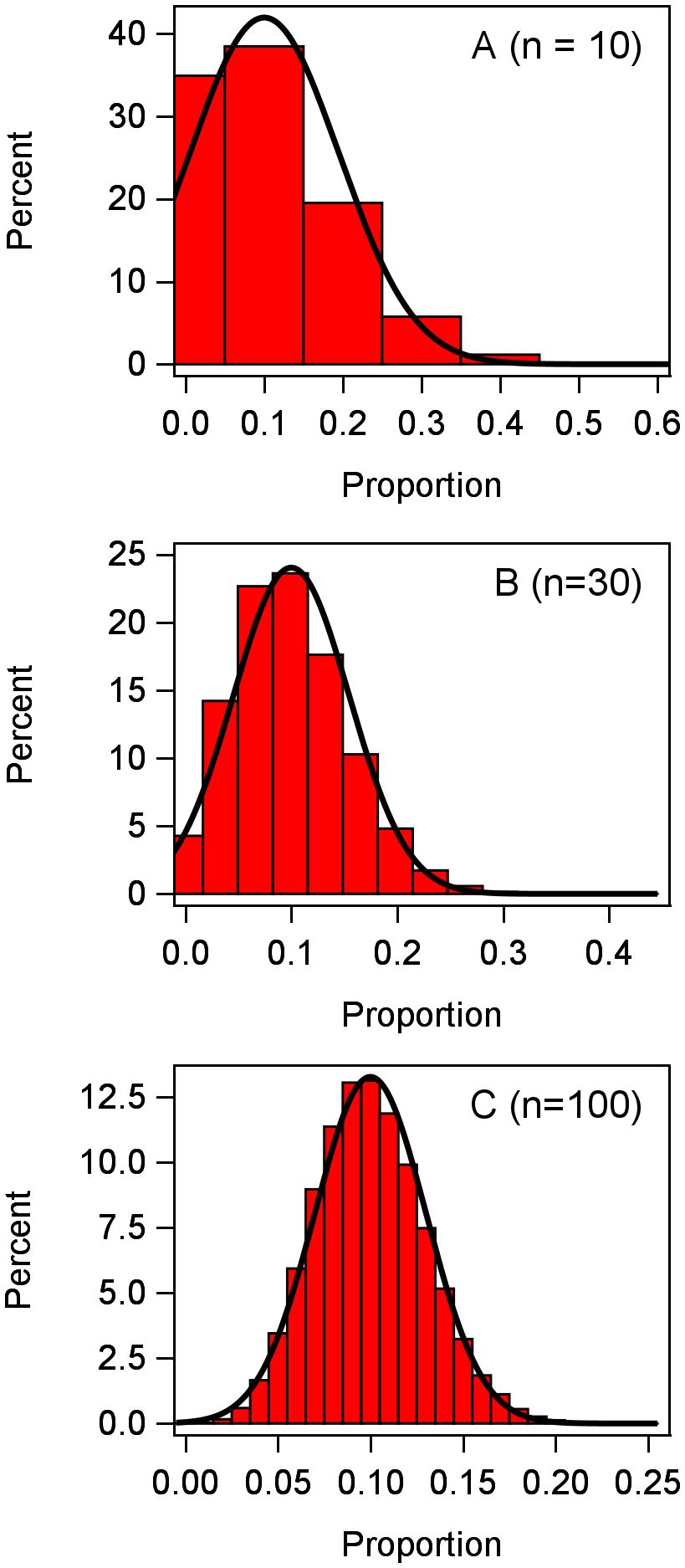
Figure 1 Frequency distribution of 100,000 observations of the response variable y generated from a binomial distribution with n = 10, 30, 100 individuals per observation. Proportions were calculated as y/n for each observation.
LMMs are not too sensitive to some departure from normality (Littell et al., 2006), and there are some LMM-fitting methods that do not require normality, e.g., MIVQUE0 (Rao, 1972), although calculations of confidence intervals and inference generally assume normality. However, even when it is reasonable to assume normality as an approximation for the binomial, the problem is that the variance of y (or of prop) will vary with the mean. The well-known angular (i.e., arcsine square root) transformation of prop does approximately stabilize variances, where prop* = sin−1(√prop) (Schabenberger and Pierce, 2002). Other variance-stabilizing transformations may be more successful when π is very close to 0 or 1 (Piepho, 2003). These may work well with LMMs (i.e., for assumed normal data), although it becomes non-trivial to interpret the exact meaning of the estimated angular means for each treatment relative to the underlying distribution of the counts (or corresponding proportions). This is especially true when there are random effects (see details and example below). There are also other challenges with the transformation-based LMM analysis. For instance, one transformation may be appropriate to stabilize variances, but a different transformation may be needed to obtain a linear (straight line) relation between y and a continuous explanatory variable (for a regression problem). Another transformation may be needed to obtain a symmetrical distribution. Thus, there are some big advantages to moving away from transformation-based analyses.
The binomial is a member of the exponential family of distributions (McCullagh and Nelder, 1989; Gbur et al., 2012; Ruíz et al., 2023). There are several other distributions of the exponential family, or have statistical properties that are very similar to those of the members of the family. These include the Poisson, NB, gamma, and beta distributions (Stroup, 2013). The binomial, Poisson, and NB are for discrete data, whereas the gamma and beta are for continuous data. GLMs and GLMMs were developed to fit data from these distributions. The normal distribution, also known as the Gaussian, is a (symmetric) member of the exponential family, so LMM can be thought of as a special case of a GLMM. We focus on the normal and binomial distributions in this paper, which are applied to discrete data. Readers should consult Stroup (2013); Ruíz et al. (2023), and Gbur et al. (2012) for details on the other distributions.
4 Models and analysis
4.1 Linear mixed model
Generically, we use y in the models as the response variable, with subscripts depending on the experimental and treatment design. For specific cases, we can use another symbol for the response. The classic LMM for a RCBD with one observation per experimental unit (ij combination) is:
where θ is a constant (intercept), τi is the effect of the i-th treatment (fixed), bj is the effect of the j-th block (random), and eij is the residual (random), the latter representing variability in the response variable not accounted for by the other terms in the model. The residual essentially gives the unique effect of each experimental unit on the response variable (after accounting for the treatment and block main effects) and is equivalent to an interaction of the treatment and block effects (when there is one observation for each ij combination, as here). The random effects for this RCBD model are assumed to be normally distributed, with means of 0 and with variances and :
Thus, Equations 1 and 2 are needed to jointly define the model for a RCBD with a random block effect. The (total) variance of yij is . In some circumstances, block could be considered as a fixed effect (Dixon, 2016), but we do not consider this here.
Equation 1 (with the distributions in Equation 2) is defined as a mixed model because beyond the fixed effect(s), it has at least one random effect in addition to the residual (Stroup et al., 2018). It is linear (in terms of the parameters and response variable y) because the terms on the right-hand side of Equation 1 are actually shorthand expressions for a sum of parameters (factor effects) multiplied by binary indicator variables that identify treatments and blocks (Milliken and Johnson, 2009) and because the left-hand side does not involve any transformation of y. Note that the fixed effects are constants (to be estimated) and the random effects are (latent) random variables to be predicted (Stroup, 2013). Many statistical programs may refer to the random effect predictions as estimates and not predictions in the output. The non-residual random effects such as blocks do not need to be normally distributed (Lee and Nelder, 1996), but this is, by far, the most common assumption. Statistical research has shown that the results often are not very sensitive to this normality assumption for the random effects (McCulloch and Neuhaus, 2011; Schielzeth et al., 2020). It is a standard assumption of LMMs that the residuals have a normal distribution. The concept of a residual substantially changes when we transition to GLMMs.
For a segue to GLMMs, Equation 1 can be rewritten in terms of expected values (means). That is, determining the expected value, E(·), of the left- and right-hand sides of Equation 1 conditional on the block random effect (more generally, conditional on all random effects other than the residual) leads to:
where μij is the so-called conditional expected value or the mean of the response for treatment i and block j. It is “conditional” because its value is for the specific level(s) of the random effect (the j-th block for this simple RCBD). From Equation 3 and the normality assumptions, the distribution of the response variable yij conditional on the random effect, yij|bj, is defined as:
Note that the mean for this conditional distribution of yij is μij and that the variance of this conditional distribution for a given block (or a given level of the random effects) is (which was given as the residual variance in Equation 2). In other words, after accounting for the fixed and random effects, the only other variability of y is captured by the variance of the conditional distribution (i.e., the unexplained variability). Readers should note that the μij in Equations 3 and 4 may be written as μij|bj in order to make the conditioning explicit (we avoid this additional notation here). Putting it all together, the alternative to Equations 1 and 2 is:
In this manner of writing the LMM, the residual term “disappears”; is now seen as the variance of the conditional normal distribution for y (after accounting for other effects). Equation 5 can actually be generalized further in a way that will help to understand GLMMs for non-normal response variables. The right-hand side of Equation 3 for the conditional mean is known as the linear predictor (LP), which is typically written with the η symbol (ηij for the RCBD here). The LP specifies all the fixed and random effects in a controlled experiment or with observational data that can affect either the conditional mean of a response variable (or a function of the conditional mean). For a LMM (i.e., normal conditional distribution), the mean simply equals the LP; that is, we link the LP to the mean with . We can then rewrite the set of equations for a RCBD as:
The LMM is rarely seen written this way, and the inclusion of the explicit LP component is excessive for this LM with conditional normal distribution; however, it does nicely allow for a transition to the non-normal conditional distributions of GLMMs. This formulation is also very useful for Bayesian model fitting because it defines the two statistical distributions in the model: the distribution of the block random effect and the conditional distribution of the response variable.
Equations 1 and 2, or Equation 6 (with the four sub-equations), can be expanded for any number of fixed and random effects, as well as the interactions of random and fixed effects (Littell et al., 2006; Stroup, 2013). Both formulations are conditional models, with the same results when fitted to data; it is just a matter of preference in how one writes the LMM. From Equations 5 or 6, the expected mean for the i-th level of the fixed effect (the i-th treatment) can be determined. The random effects are integrated out to obtain μi (instead of μij). Because the expected value of the normally distributed bj is 0, the result for a LMM is simply:
This is generally of most interest to the investigator. The estimates of μi and the differences of μi between treatments (μi − μi′, where i and i′ are any two treatments), as well as their SEs (a function of the variances in Equation 6), are derived from statistical theory and are automatically calculated with LMM software (with the right statements or options). Details are in mixed-model textbooks (e.g., Littell et al., 2006; Galecki and Burzykowski, 2013; Stroup et al., 2018).
There is yet another way to write a LMM. The two random-effects terms (including the residual) in Equation 1 can be taken and combined into one term as: hij = bj + eij. The LMM can then be written as:
This LMM is known as a marginal model for a RCBD experiment (Stroup, 2013). Both block and residual effects are still present, just expressed differently. The variability component(s) now has to be written with more complexity to express both random sources. The approach is to define a vector of random effects for each level of the random effect (the j-th block here), designated hj. In order to save space, we assume here that there are just three treatments, so we can write:
where each element of the vector corresponds to a different treatment. This leads to the derivation of the variance–covariance matrix (P) for yij:
The diagonal elements of the matrix are the (total) variances of yij (; the same for each treatment), while the off-diagonal elements () are the covariances of the response variables. This formulation helps to make clear that, with a random block, observations that are from the same block are correlated. The correlations within a block can be determined from the covariances and variances (Littell et al., 2006). This structure is known as compound symmetry (CS). The conditional model (Equations 1 and 2, or Equations 5 or 6) and the marginal model (Equations 8 and 10) are equivalent for LMMs. Fitting either version will give the same result when fitted to data if is 0 or positive. Although the conditional model in Equations 5 or 6 does not explicitly show a covariance, the covariances between treatments are still there, derivable from the terms of the conditional model. For the RCBD, the correlation of yij within the same block (say, j = 1), known as the intra-class correlation, is:
The reader can find more details in Stroup (2013) and Gbur et al. (2012).
The most common method to fit LMMs is through the use of restricted maximum likelihood (REML), also known as residual maximum likelihood. This can be considered the gold standard. REML produces unbiased parameter estimates (such as with a RCBD) or less biased estimates than those produced with maximum likelihood (ML). Bayesian methods can also be used (Wolfinger and Kass, 2000; Stroup, 2021), as well as some alternative frequentist approaches (Littell et al., 2006). It is important to note that, whether the data analyst uses the conditional (Equation 6) or the marginal (Equations 8-10) form of the LMM, the actual (observed) data correspond to the marginal distribution (Gbur et al., 2012). In essence, the conditional and marginal models are just two different ways of generating data from a marginal distribution (Stroup, 2013). The random effects in a conditional LMM are random latent variables that are not directly measured or observed; rather, they are predicted through the model-fitting procedure. What one observes (measures) and then analyzes are data arising from the marginal distribution, no matter how that marginal distribution is derived or generated.
4.2 Example data analyzed with LMMs
Using the GLIMMIX procedure in SAS with REML estimation, the conditional LMM in Equation 6 (equivalent to Equations 1 and 2) was fitted to the example data with the proportion of diseased wheat spikes as the response variable (propij for yij). This is not normally done as the variance is not independent of the mean for binomial data (or discrete data, in general). Estimates of the treatment means (e.g., ) and the SEs are given in Table 1, together with one pairwise difference of means. The exact same results are obtained if the marginal model (Equations 7–10) is fitted for this LMM (results not shown). The SEs are functions of the block and residual variances (details in Gbur et al., 2012; Stroup, 2013). Interestingly, despite the problems in directly analyzing proportions, the estimated mean proportions from the fitted LMM are unbiased estimates of the true proportions for each treatment across all the blocks (i.e., across all the levels of the random effects; the marginal means) (Stroup, 2013, 2015). However, the estimated SEs across all treatments (0.0590) are meaningless because the LMM assumes a constant variance (). Since the estimates of variability are wrong, the estimates of confidence intervals and the tests of significance are thus wrong.
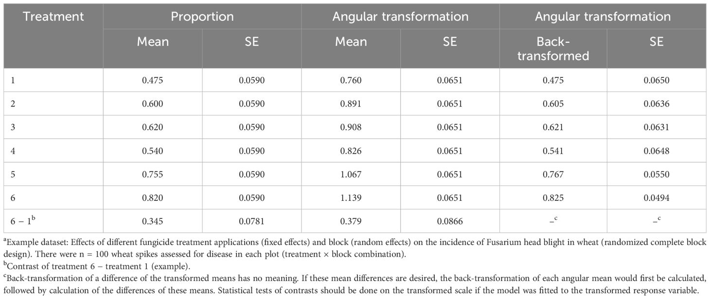
Table 1 Estimated means and standard errors (SEs) when fitting a linear mixed model (LMM; Equation 6) to the proportion of diseased wheat spikesa with an incorrect assumption that the residual variance is constant (i.e., independent of the mean proportion) and when fitting the LMM to the angular transformation of the proportions where it is reasonable to assume the transformed values have constant residual variance, together with the back-transformation of the estimated angular means to obtain proportions (where the SE of the back-transformation is based on the delta method).
The LMM of Equation 6 can be generalized to allow for a separate residual for each level of the fixed effect (). This is easily done using REML algorithms such as in the MIXED procedure in SAS. Fitting such a model can be more challenging, especially with the small sample sizes typically found in agricultural field studies. With the number of blocks in this example being four, attempting to estimate each treatment-specific residual variance is thus not a good strategy.
The results of fitting the LMM to the transformed angular data are also shown in Table 1. The estimated SEs were constant across the treatments (0.0651), which is expected since one assumes that the angular-transformed data have variances independent of the mean. Comparisons of the treatments and tests of significance can be done on these mean transformed values, and back-transformation of the means can be performed to obtain a type of “mean proportion” for each treatment, as shown in the table. However, it is not intuitive what these back-transformed means represent exactly. They are not estimates of the means of the distributions of the actual proportions, but are related to those means.
In symbols and suppressing subscripts here, using g(y) as a transformation (function) of y [such as a log and angular (arcsine square root), among others], the expected value (i.e., mean) of g(y), E(g(y)), is not equal to the transformation of the expected value (mean) of y, g(E(y)) (Schabenberger and Pierce, 2002). These two types of means are related, but are not the same. The situation becomes even more complicated with multiple random effects. For the example (Table 1), the back-transformed values give a type of “central” (but not truly central) value of the marginal distribution of the data. Nevertheless, analytical approaches based on transformations still have value, as long as the investigators understand the limitations.
5 Generalized linear mixed models
5.1 Conditional non-normal distributions
With GLMMs, investigators have the opportunity to better match the model used for data analysis with a plausible model for stochastic generation of the data (Stroup, 2013, 2015). Consider the disease incidence data in the example, where it is reasonable to assume a binomial distribution for y in a given plot (experimental unit), at least as a starting point. Suppressing subscripts temporarily, we can write generically, y|plot ~ Bin(π,n), for the conditional distribution of the number of diseased wheat spikes (this could also be for the number of germinated seeds in a pot in a greenhouse, etc.). The probability of disease (or the probability of some trait), π, could be influenced by the pathogen inoculum density, the favorability of the environment for infection, and so on. It is quite plausible that π represents a parameter that has direct mechanistic interpretation. We continue with our hypothetical example from Figure 1 and consider π = 0.1 (following closely, once again, the method in Stroup, 2013).
Consider the impact of random effects, such as blocks. If there is only one treatment (e.g., control), then the plot and the block are synonymous. With random effects, π is randomly perturbed by the block, so that π is higher than 0.1 in some blocks (plots) and is lower than 0.1 in other blocks. The response y in each block (for any single treatment) would depend on the realized value of π for that block. On average, the perturbation is 0, at least on one possible scale. Ultimately, we want to specify the marginal distribution of y [across the population of plots (blocks)] based on the data-generating process in each plot (block) and the distribution of perturbations across the plots. A linear additive scale for the perturbation of the random block effects (i.e., adding bj directly to π) would not work in a realistic model, in general, because a random permutation could give a probability nonsensically above 1 or below 0 in a given plot when π is relatively close to 1 or 0. A linear perturbation could work on a function of π, if the right function was used, so that π remains bounded by 0 and 1. This is the approach taken in the usual GLMM.
Being more explicit and referring back to the conditional distribution form of a LMM (Equation 6), we can write the LP for a RCBD as . This is exactly the same for a normal or a non-normal conditional distribution. Likewise, the random block effect can be assumed to have a normal distribution, as with LMMs. The question is how to link the ηij LP to the location parameter. This is done through the link function, g(πij), or, more generally, as g(μij), where a link function is a transformation of a parameter (not a transformation of the observations). Thus, we can write g(πij) = ηij. The location parameter is obtained by the inverse link function, written as πij = g−1(ηij) = h(ηij). For conditional binomial data, the logit is the most common link function; that is, g(πij) = logit(πij) = ln(πij/(1 − πij)). There are other possibilities for the link function based on specific applications or theory (Collett, 2003). The term “identity link” or “identity link function” is used when there is no transformation of μ or π.
For a RCBD (one fixed-effects factor and random block effect factor), we can now write the conditional model form of the GLMM generically as:
where “Dist” is generic for some conditional distribution. This equation is almost the same as that for the LMM (see Equation 6). For conditional binomial data (with π = μ), in particular, we write:
Recall that the mean of the binomial is nπ for y; the mean of y/n is π. Thus, the location parameter π with the binomial plays the role of μ in the general distribution (Equation 12). Unlike with a LMM, it is important to note that there is no variance to estimate for the conditional binomial distribution (i.e., no unknown residual variance as the variance of the binomial is fully defined based on n and π). The variance of the conditional binomial is nπ(1 − π). See GLMM expansions and extensions below (Section 6) for the implications of this. One can reduce Equation 13 to three components by directly writing as the first sub-equation. It is important to note that, although the g(·) link function is a transformation, a GLMM is not a model for a function or transformation of data (i.e., not a model for the transformed response variable). Put another way, a GLMM is not a model for the mean of transformed observations; rather, it is a model for a function (transformation) of the mean (μ, π, etc.) of the actual (non-transformed) observations. This subtle difference is extremely important. The LP of the GLMM in Equation 13 estimates a function of the probability of disease for a particular treatment and block. The inverse link to obtain π for a logit link function is given by:
5.2 Marginal distribution
Integrating over the random effects of the conditional LMM (Equation 6) results in the marginal distribution for y (Littell et al., 2006; Stroup, 2013; Brown and Prescott, 2015). With normality for the random effects and the conditional distribution in a LMM, the marginal distribution is determined analytically. The expected values of the fixed effects of this marginal distribution (e.g., ) are the same as those obtained simply by inserting 0 (the expected value of the normally distributed random effects; see Equation 2) for the random effects in the conditional LMM (Equation 3).
The situation is different with GLMMs. The marginal distribution cannot be determined analytically, requiring numerical integration; for the binomial conditional distribution, as an example, is not the logit of the mean proportion of diseased individuals over all the blocks (i.e., over all the levels of the random effects). This is because the inverse link is a nonlinear equation (Equation 14) and the conditional distribution is not normal. This is an extremely important concept because, as discussed above, one observes the marginal distribution (more technically, a sample from the marginal distribution), not the conditional distribution. Numerical integration over the random effects can give an estimate of the marginal distribution (required for model fitting), including estimates of the marginal mean (the marginal mean proportion of diseased plants here over all the blocks) and its variability. This is explained by Stroup (2013) on pages 102–107 for a similar situation. Sometimes, this marginal distribution, which is made up of the mixture of the binomial and normal distributions, is called the logistic–normal–binomial (LNB) distribution when used to characterize the spatial variability in fields (Hughes et al., 1998).
The marginal distribution from Equation 13 can also be obtained by simulation for known parameters for the conditional distribution and the random-effects distributions. Following Stroup (2013) closely, we estimated the marginal distribution of the diseased proportion (y/n) across levels of the random effects by simulating 100,000 observations from Equation 13, with π = 0.1 and n = 30 for the conditional binomial distribution, and three levels of the block effect standard deviation [ = 0.5, 1.0, and 1.5 ( = 0.25, 1.0, and 2.25)]. With simple random sampling (i.e., no random effect distributions), the binomial distribution is not very skewed with n = 30 (Figure 1). However, in a mixed-model setting with symmetric (normal) random effects, the marginal distribution of the proportion can be very skewed depending on the value of the block variance. As seen in the left-hand column of Figure 2, the marginal distribution becomes more and more skewed with increasing block variance. A general rule of thumb is that marginal distributions are not symmetrical for GLMMs, with the skewness dependent on the skewness of the conditional distribution (e.g., binomial) and the magnitude of the variances of all the random effects in a LP.
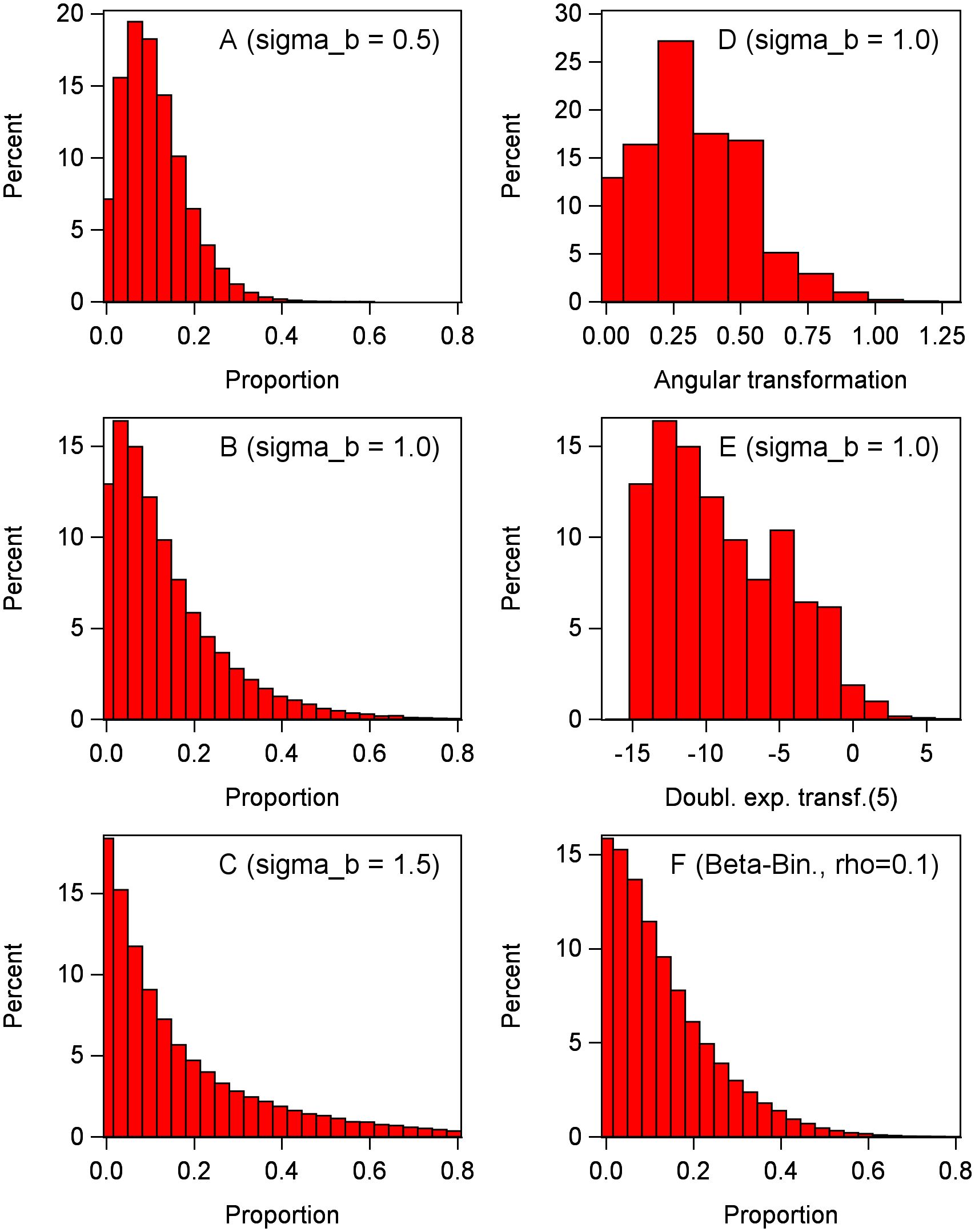
Figure 2 Marginal distributions determined by generating 100,000 observations of the response variable y with a conditional binomial distribution (with π = 0.1 and n = 30 individuals per observation), plus a random effect for each observation (which had, for most graphs, a normal distribution with variance of or standard deviation of ). Inverse link is used to obtain y from logit(π). Proportion is calculated as y/n. Left-hand column: (A–C) Data generated with Equation 13 (without τ because there is only one treatment, with bj now as a plot effect), with standard deviations of bj effect of 0.5 (A), 1.0 (B), and 1.5 (C). Right-hand column: (D) Data generated as in (B) (standard deviation of 1), but the proportions transformed with angular transformation. (E) Data generated as in (B) (standard deviation of 1), but the proportions transformed with Piepho (2003) function (with δ = 5). (F) Unlike other graphs, y is generated with beta-binomial distribution with overdispersion parameter of = 0.1 and no bj effect, approximately giving the same variance of y/n as in (B) (with a standard deviation of 1).
In the simulation example in Figure 2, the mean proportions of the marginal distributions are estimated as 0.109, 0.134, 0.169 for block variances of 0.25, 1.0, and 2.25, respectively, all with π = 0.1 (displayed in Figures 2A–C, respectively). That is, the mean proportions increase with increasing random effect variances even though the underlying location parameter for the conditional distribution (i.e., for the generation of observations in each experimental unit) is fixed at π. Broadly, the mean proportion will not correspond to the inverse link of θ + τi for treatment i (or just θ when there is just one treatment). When π is less than 0.5, the marginal mean proportion will be greater than π, with the degree of difference being dependent on the random effect variability. When π is greater than 0.5, the marginal mean proportion will be less than π. The variances of the marginal distributions also increase in the same manner. Using the angular transformation of the observations in a LMM does not lead to a symmetric marginal distribution, as seen in Figure 2D for an example block variance of 1.0. The new variance-stabilizing transformation of Piepho (2003),
with a stabilizing parameter of δ = 5 also does not lead to a symmetric distribution when the block variance is 1.0 in this example (Figure 2E). We estimated δ using the ML methodology in Piepho (2003) (results not shown). Other tested values of δ did not result in a symmetric distribution. As discussed by Piepho (2003), the new variance-stabilizing transformation to be used in LMMs is very effective in stabilizing variances (among treatments), but is less effective in producing a symmetrical distribution of the transformed data (especially when the original distribution of y is very skewed).
There are other ways to derive a marginal distribution than the typical method here of mixing a normal random effect distribution with conditional binomial on the link scale. For example, it is well known that the beta-binomial provides an excellent representation of the distribution of disease incidence when there is overdispersion (i.e., higher variability than for the binomial alone, sometimes called extra-binomial variation) (Madden and Hughes, 1995; Turechek and Madden, 1999; Madden et al., 2007). In general, the beta-binomial is utilized to characterize the spatial variability (clustering) of incidence within fields, where each sampling location in a field is a separate observation of disease incidence (based on n observed units for each sample) (Turechek and Madden, 1999), but the concept is easily extended to variability among blocks in planned experiments. In the context of a RCBD, the beta-binomial is derived by, once again, assuming that π is randomly perturbed in each plot (block, etc.). However, the random block effect is not additive on the link scale of the binomial [e.g., not adding bj to the equation for logit(πj)] as it is for the derived GLMM of Equation 13. Instead, the random block effect is assumed to have a beta distribution and is multiplicative with π (i.e., working directly on the scale of π) (Madden and Hughes, 1995). The plot effect is characterized by a correlation parameter (instead of ). An example of simulated observations from a beta-binomial distribution is shown in Figure 2F, where was chosen to roughly have the same effect as = 1 with the normal random effect (Figure 2B). As with the other scenarios in Figure 2, the marginal distribution is very skewed here.
There are many uses of the beta-binomial and the related binary power law (Hughes and Madden, 1995; Madden et al., 2018), but the beta-binomial is not commonly used for routine data analysis with GLMMs (e.g., determining treatment effects). Since the random effect is considered non-normal, the beta-binomial is a special case of what is often called doubly (or double) generalized linear mixed models (DGLMMs) (Lee et al., 2006). We consider this in some more detail below.
The key question in a GLMM is the measure of the “location” (and associated SE) one wants to estimate. In agreement with Stroup (2013, 2015) and Stroup et al. (2018), we argue that for conditional binomial data, one wants to estimate logit(πi) = θ + τi for treatment i and the conditional probability πi using the inverse link function (location parameter of the conditional binomial) (Equation 14). That is, one is interested in the parameter from the conditional distribution, the probability of disease when the random effects are exactly at their means (0). This is considered a conditional mean. This location parameter is not affected by the distribution of the random effects [although the random effect variances do affect parameter estimation and the precision (SE) of parameter estimates]. It turns out that the πi from the conditional binomial (for treatment i) is the median of the marginal distribution of proportions for this treatment (Stroup, 2013). Most importantly, when the GLMM of Equation 13 is fitted to RCBD data, estimates of logit(πi) for each treatment (θ + τi), and therefore πi through the inverse link (Equation 14), can be directly obtained.
5.3 Example
The estimates of the logit of the probability of disease and the corresponding conditional probabilities (inverse links), together with their estimated SEs, from the fit of Equation 13 are given in Table 2 (listed as model A). This is based on restricted pseudo-likelihood (RSPL) model fitting, discussed below. As expected, the SEs are not equal for the different treatments, being a function of the variance of the conditional binomial and the block variance. The block variance estimate was small in this example ( = 0.073), and the proportions are not very close to 0 or 1, meaning that the of the conditional binomial (based on the inverse link) is close to the mean proportion of the marginal distribution obtained with the fit of the LMM to the proportion data (Table 1). However, the SEs vary greatly between the LMM and GLMM approaches [e.g., 0.042 for treatment 1 with the GLMM (model A in Table 2) versus 0.059 for the same treatment with the LMM (Table 1)], reflecting that the GLMM properly accounted for the variance of a binomial distribution and estimated a conditional distribution parameter.
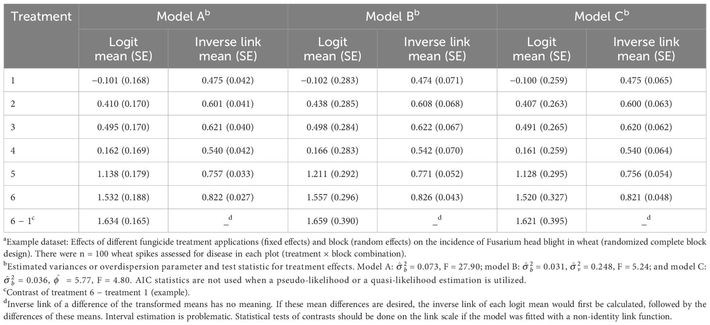
Table 2 Estimated means and standard errors (SEs, in parentheses) both on the linear predictor scale [logit(mean)] and the data scale (inverse link; with SEs based on the delta method) when fitting three generalized linear mixed models (GLMMs) using restricted pseudo-likelihood (models A and B) or restricted pseudo-likelihood with a quasi-binomial conditional likelihood (model C) to the number of diseased wheat spikesa: naive Equation 13 (model A); Equation 16, which includes an additive random effect for the individual experiment unit (plot; model B); and Equation 17, which includes a multiplicative overdispersion parameter instead of an additive experimental unit effect (model C).
6 GLMM expansions and alternatives
6.1 Link functions
Although it is very common to use the logit link with a conditional binomial distribution in a GLMM, there are other choices, such as the probit (inverse standard normal function) and complementary log–log (CLL) [ln(−ln(1 − π))]. There may be theoretical reasons to choose a different link for some applications (Collett, 2003), or selection may be based on the goodness of fit of the model (Malik et al., 2020). For instance, Kriss et al. (2012) used the CLL link in a hierarchical GLMM for surveys of clustered plant disease incidence data, where the choice of link was based on previous theoretical and empirical work on the relationship between disease incidence and severity (a continuous variable) and the relationship between incidence at two (or more) scales in a spatial hierarchy (Turechek and Madden, 2003; Hughes et al., 2004; Paul et al., 2005). Many other possible link functions have been proposed, and Malik et al. (2020) described several of them, with a proposed approach for deciding on an appropriate link to use.
The reason for the logit being the default link has to do with the form of the binomial distribution. One method of writing the log of the binomial distribution (derived after a little algebraic manipulation of the function typically given in introductory statistics courses) is:
Equation 15 is in the form for a member of the exponential family of distributions (Collett, 2003; Gbur et al., 2012). A key property of this family of distributions is that there is a term that involves the product of the response variable (y) and a so-called canonical parameter, which is either the mean (expected value, μ) or the location parameter, or a function of the mean for the distribution. Here, the canonical parameter is the logit of π, ln(π/(1 − π)), the typical link function for the binomial. For the Poisson, for instance, the canonical parameter is ln(μ), which is the typical default link function for count data. The work by Gbur et al. (2012) and many of the major reference books for GLMMs give the ln[f(y)] forms for other distributions or density functions in the exponential family. All the relevant properties of these distributions (such as the variance, among others) follow directly from the form of the ln[f(y)]. When the default canonical link is not selected, the main software programs, such as GLIMMIX in SAS, handle the necessary extra calculations in the background to fit models and calculate statistics.
6.2 Realistic modifications of the GLMM
The GLMM with a binomial conditional distribution (Equation 13) is the obvious natural extension of the LMM (Equation 6) for a RCBD; however, there is a very good chance that the use of the simple GLMM with agricultural (or other) experiments will give incorrect results! In particular, the SEs of the estimated location parameters (μ and π) for treatments (on the link scale of the model or for the inverse link scale of the data) may be too small. Likewise, tests of significance are likely to be wrong or misleading, where the test statistics are too large and the p-values for significance too small (Stroup, 2015). This is an important warning, as elaborated below. To understand this, note that the conditional normal distribution in Equation 6 has a variance () that is estimated, but there is no variance to estimate with the conditional binomial. The variance of y for a conditional binomial distribution is fully defined by π and n; that is, var(yij|bj) = nπij(1 − πij) for the RCBD with random block effect. However, as discussed elsewhere, count data are very commonly overdispersed (Madden et al., 2007, 2018); that is, y has a higher variance at the experimental unit (plot) level than nπij(1 − πij). Similarly, for counts without an upper bound, y has a higher variance at the plot level than the theoretical variance for a Poisson distribution (μ) (Madden and Hughes, 1995; Madden et al., 2018). As an aside, the concept of overdispersion as used here does not exist for the (conditional) normal distribution because the residual variance is independent of the mean; can take on any value to account for the variability not accounted for by the other terms in the model (in other words, the residual variance is estimated from the data). For plant diseases, there are numerous causes for overdispersion at the experimental unit (plot in this case) level, especially the clustering of diseased individuals in plots or fields (Hughes and Madden, 1995; Madden et al., 2007). More broadly, any non-uniformity within the experimental units or nonrandom sampling of the units, or misspecification of the LP (right-hand side of the equation for η), or misspecification of the conditional distribution in the model can result in overdispersion in a given data analysis. Put another way, overdispersion can occur “when the model fails to adequately account for all the sources of variability” (Stroup et al., 2018, p. 391).
There are multiple ways to deal with overdispersion when analyzing discrete data. The primary approaches for our purposes in this article are: 1) to expand the LP to include an additional random-effects term (or terms); 2) to use a quasi-likelihood for the conditional distribution; or 3) to use a different conditional distribution that allows for higher variability than for the binomial (or Poisson for unbounded counts) (Stroup, 2013). There are important implications for all of these model expansions in terms of model fitting (estimation). We defer the discussion on estimation until later.
6.3 Adding terms to the linear predictor
The first of these approaches is the expansion of the GLMM. For the RCBD conditional model of Equation 13, we add a term for the interaction of block and treatment, (bτ)ij, which we can write as vij, to the right-hand side of the LP:
The distribution of vij is assumed to be normal, . Now, the conditional distribution of y given the random effects is written as:
Conceptually, we assume that π is randomly perturbed not only by the block but also by the individual plot. Recall that the residual term in Equation 1 for a normality-based LMM is equivalent to the interaction of block and treatment, where the residual term accounts for the variability not accounted for by the other terms in the model. Therefore, the expansion of the LP for the conditionally binomial data is in the same spirit, taking into account the experimental design [for experiments without blocks, the bj term would not be present, but the vij term would still be used here for the random effect of the experimental unit (plot)]. For the RCBD with conditional binomial data, Equation 13 is now written as:
The same general approach is used for any conditional GLMM that is based on a conditional binomial or a conditional Poisson distribution (with any number of fixed and random effects), i.e., to add a residual-like random effect to the LP equation of the model. This may be a three-way or a higher-order interaction, generally a crossing of all the terms in the LP. Equation 16 is considered a conditional model, and the πij represents the probabilities of disease for the individual plots (combination of treatment and block), the same as with Equation 13. Interest still remains on the estimation of logit(πi) (= ) and, hence, πi.
6.3.1 Example
Fitting Equation 16 using RSPL (see below for a discussion on model fitting), which we label as model B, resulted in estimates of = 0.031 for block (compared with 0.073 for model A) and = 0.248 for the block × treatment interaction [plot random effect (“residual”)] (Table 2). Although the block variance is smaller than that of the naive GLMM above (no vij term), there is now a nonzero plot variance that was not previously considered. The estimates of the LP (logit) and the inverse link for each treatment are shown in Table 2. Here, the estimated SEs are larger than that for the fit of the simpler Equation 13 (e.g., 0.283 for treatment 1 logit for Equation 16 versus 0.168 for Equation 13). This, together with the nonzero estimated variance for vij, is an indicator of the overdispersion that needed to be accounted for. The F statistic for treatment significance is now 5.24, smaller than that for the simpler (and inadequate) Equation 13 that did not account for the extra variability (F = 27.9). The means (on the link or data scale) are similar to the results found using the simpler model. However, these means will, in general, not be the same.
6.4 Quasi-likelihood
When there is greater variability than is possible with a binomial distribution (i.e., with overdispersion or extra-binomial variation), instead of adding a random effect term as the LP, the conditional variance can be defined as a constant times the binomial variance. For a RCBD, this is var(yij|bj) = ϕnπij(1 − πij), where ϕ is an overdispersion scale parameter. It plays the role of the index of dispersion (D) in spatial pattern analysis (Madden et al., 2018). By allowing ϕ to take on any positive value, the conditional variance can always be expressed as a multiple of the binomial. For unbounded counts, one would write var(yij|bj) = ϕμij, where μij is the variance (and the mean) of the Poisson distribution. With ϕ not equal to 1, the conditional distribution is no longer binomial; in fact, there is no longer an actual true conditional statistical distribution that could stochastically generate the data. Thus, one has a so-called quasi-likelihood, and a method suitable for quasi-likelihood is used to fit the model (Gbur et al., 2012; Stroup, 2013). See below for a discussion on estimation.
The quasi-likelihood-based model for the RCBD is given as a slight modification of Equation 13:
where is an arbitrary expression that represents a conditional quasi-likelihood (which is not for the actual distribution of the data). Note that the LP (ηij) is the same as the naive GLMM in Equation 13 (i.e., no addition of a vij term). It would be incorrect to add the vij term (block × treatment interaction) in a model where the ϕ is also added as this would be overparameterization; that is, two terms ( and ) would be “competing” to explain the overdispersion.
6.4.1 Example
Table 2 displays the estimated means and SEs (model-scale logits and data-scale inverse link means) for the fit of Equation 17 based on the conditional quasi-binomial likelihood (model C). This was done with RSPL (see below). The estimated means are extremely close to those obtained for the fit of naive Equation 13 (model A), but the SEs are much larger, reflecting an estimated scale parameter of = 5.77 (i.e., the conditional variance is nearly six times larger than that obtainable with the binomial). The SEs are all larger than those for the fit of the naive Equation 13, but more similar to the SEs for the expanded LP model of Equation 16 (model B). The test of treatment effect is now F = 4.80, similar to that obtained with Equation 16 and much smaller than the F for the naive Equation 13 (model A).
The use of quasi-likelihood for model fitting is very straightforward and can be applied to many modeling situations. It is often considered a simple fix for overdispersion in GLMs or GLMMs (McCullagh and Nelder, 1989). Nevertheless, (Stroup 2013, pp. 347–348) was somewhat critical of the approach because an actual likelihood function is not used in the estimation as there is no true conditional distribution. That is, there is no model for the direct stochastic generation of the data. There are alternative approaches, such as the use of Equation 16 (model B), which may be consistent with the experimental design (i.e., random block and plot effects in this example). Model B (Equation 16) can be thought of as characterizing one possible data generation process for the given experimental design (e.g., the random effects of blocks and experimental units such as plots) and model C (Equation 17) as characterizing a consequence of the random effects affecting π (or μ in general) that are not in the model. Piepho (1999) and Madden et al. (2002) compared these and other GLMMs for the analysis of plant disease incidence data. Piepho (1999) should also be consulted for a more thorough discussion of data generation processes that would lead to model B or C.
6.5 Different distributions with overdispersion
For unbounded count data, Poisson is commonly replaced by the NB to account for overdispersion at the experimental unit level (or for the clustering of individual observations, in general) (Madden et al., 2007). The conditional Poisson would be replaced with the conditional NB in Equation 13. Because the NB has its own overdispersion parameter k that is estimated, then a vij term would not be added and a ϕ not specified for a quasi-distribution. This substitution of the NB for the Poisson is easy to do with the GLIMMIX procedure in SAS. For overdispersed binomial-type data (when there is an upper bound of n for y), such as in our example, the beta-binomial distribution (“Betabin”) can replace the binomial. This distribution is not in the exponential family and is much less used for mixed-model analysis, although it has had more use with GLMs with only fixed effects (Hughes and Madden, 1995; Morel and Neerchal, 2010) and for quantifying aspects of the spatial heterogeneity of plant diseases (Madden et al., 2007, 2018). To use this model, the in Equation 13 would be replaced with , where is one formulation of the overdispersion parameter for this distribution (at = 0, the Betabin reduces to the binomial; as increases, overdispersion increases). The LP would contain only the treatment and block effect (as in Equation 13). This can be considered one type of DGLMM (Lee et al., 2006).
The beta-binomial distribution is not available in the GLIMMIX procedure, but can be fitted using ML (not the REML) with the NLMIXED procedure when there are random effects (such as block effects). Considerably more coding is required to achieve this for the beta-binomial. An alternative to fitting the beta-binomial is to utilize the h-likelihood (see below).
The results for the example with the beta-binomial as the conditional distribution (model D) are given in Table 3 based on ML estimation. Although the means are similar, the SEs are larger than those for model A (Equation 13) as the extra-binomial variability is taken into account, but smaller than those for models B and C (which take into account the extra-binomial variability in different ways). The smaller SEs for the beta-binomial are due, in part, to ML rather than REML being used in the estimation.
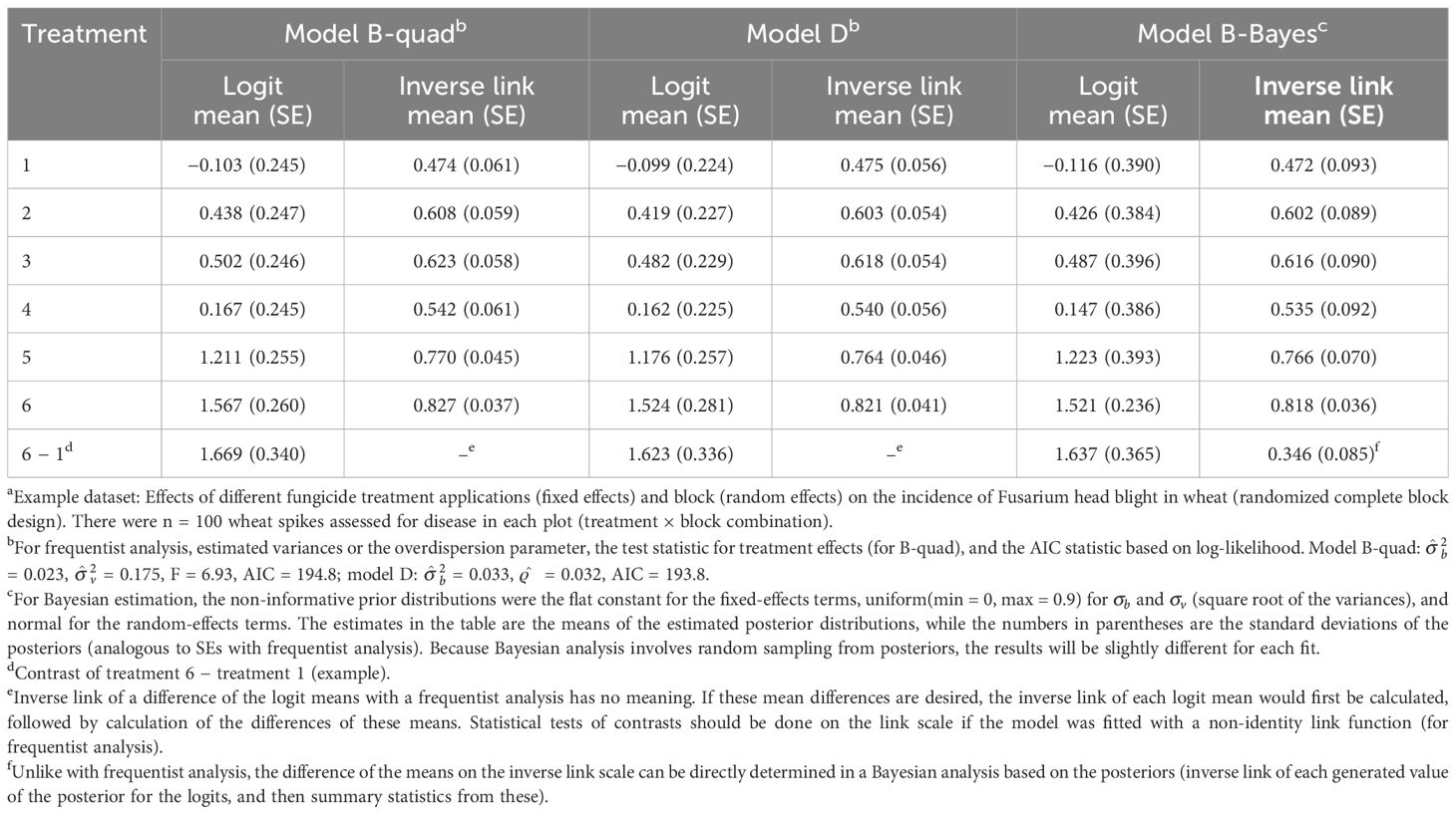
Table 3 Estimated means and standard errors (SEs, in parentheses) both on the linear predictor scale [logit(mean)] and the data scale (inverse link; with SEs based on the delta method) when generalized linear mixed models (GLMMs) were fitted to the number of diseased wheat spikesa using maximum likelihood with the quadrature method for integral approximation for Equation 16 (model B-quad), for Equation 13 but with the beta-binomial for the conditional distribution of y instead of the binomial (model D), and when using Bayesian estimation with Equation 16 (model B-Bayes).
7 Fitting GLMMs to data
Unlike with normality-based LMMs, the method for fitting GLMMs to data (i.e., parameter estimation and random effects prediction) is controversial (Stroup, 2013; Stroup and Claassen, 2020). Even the labels for the model-fitting methods are confusing and are used differently by different researchers, with the labels even evolving over time. For LMMs, REML is the generally preferred (and noncontroversial) method of model fitting, partly because it produces unbiased estimates (fixed effects and their SEs) or less biased estimates than ML (McCulloch and Searle, 2001; Galecki and Burzykowski, 2013; Stroup et al., 2018). For simple cases, REML duplicates the results for the mean square (and moment)-based methods that predate the contemporary likelihood-based methods for LMMs. Regular ML can also be used for LMMs. However, it is well known that this produces biased estimates; in particular, the variance estimates and the SEs will be too small for ML estimation, resulting in the test statistics being too large. The latter is an issue when the number of independent observations is small. REML and ML are both iterative methods, although simple situations can result in convergence in a single iteration.
Recall that, for any experiment or survey, the observed data are a manifestation of the marginal distribution. Thus, the estimation requires integration over all the random effects in a conditional model to approximate the marginal distribution. However, there is no analytical solution (i.e., mathematical expression) for this integration with GLMMs; only approximations are possible, which is one of the complexities of working with this class of models. In fact, practical use of GLMMs only became possible with the availability of fast computers with large memory (and excellent programming). Despite the many labels in the literature, two broad frequentist methods can be used: model approximation (linearization) and integral approximation. There are also some more specialized methods.
7.1 Linearization
Linearization involves a first-order Taylor series expansion of the inverse link function of the LP equation [πij = g−1(ηij) = h(ηij)], generally centered on the current (or initial) estimates of the fixed and random effects (Breslow and Clayton, 1993; Wolfinger and O’Connell, 1993). A so-called pseudo-variable (y*) is formed based on this expansion, which is a function of the current parameter estimates (and random effect predictions) and the first derivative of the inverse link with respect to the LP. The expected value of y* is modeled as a function of the fixed and random effects (the right-hand side of the LP). The variance of y* conditional on the random effects is a complex function of the first derivatives and the variance function for the conditional distribution [e.g., nπ(1 − π) for binomial and μ for Poisson].
Wolfinger and O’Connell (1993) developed a pseudo-likelihood (PL) method based on linearization. The PL method makes the (approximating) assumption that the conditional distribution of y* (but not y), given the random effects, is normal with a complicated variance (Stroup, 2013; Xie and Madden, 2014). As a consequence, the marginal distribution is also normal. Thus, one can use the machinery of normality-based LMMs to fit GLMMs and then (automatically) recover the relevant statistics for the actual distribution of y after convergence of the PL algorithm. The PL fitting algorithm is doubly iterative in that the fitting of the y* pseudo-variable is iterative (as is any LMM), and then the y* is updated at the end of each LMM fit based on the LMM results, with the LMM fitting being repeated with the updated y*. The double iterations continue until convergence (defined in different ways). With PL, one ultimately is basing the analysis on the actual distributions specified in the model for y (the normality assumptions for y* is only for the intermediate computational work). Restricted PL is the default in the GLIMMIX procedure in SAS (called RSPL in SAS), which uses REML-based model fitting for the pseudo-variable. As an option, the ML version of PL (ML-based PL; known as MSPL in GLIMMIX) can be performed. An overdispersion term, ϕ, can also be added as an option (see Equation 17) with the PL method (either RSPL or MSPL), which then becomes a quasi-likelihood approach (no longer a true statistical distribution for the conditional distribution of y). We are not aware of any R packages for PL estimation.
Breslow and Clayton (1993) took a quasi-likelihood approach, which only assumes that the objective function to maximize in the iterative estimation process has the general form of a member of the exponential family of conditional distributions (defined through a mean and variance, but with a multiplicative overdispersion parameter). This approach is often labeled as penalized quasi-likelihood (PQL) or marginal quasi-likelihood (MQL). Implementation in R can be done with the “glmmPQL” function in the MASS package. In this program, the overdispersion parameter ϕ is always estimated (cannot be restricted to 1); therefore, the results do not correspond to a (conditional) distribution for y, but to a quasi-likelihood. The PL approach taken to fit model C in the example (Table 2) has analogy with the PQL method of Breslow and Clayton (1993).
The PL method is extremely flexible, allowing not only true distributions but also quasi-likelihoods and can easily handle correlated observations, such as in temporal or spatial repeated measures (Stroup, 2013). The RSPL method was therefore used to fit models A, B, and C to the example data discussed so far.
7.2 Integral approximation
Instead of approximating the model to obtain a marginal distribution of a pseudo-variable, the integration over the random effects (of the original model) can be approximated to obtain an estimated marginal distribution of y. Generally, the best method to use is the Gauss–Hermit quadrature (quadrature for short), although it is computationally demanding and can be extremely (or painfully) slow for moderate to large data problems, sometimes requiring many hours if there are several factors and interactions. The Laplace approximation, a special case of quadrature, is another integral approximation method that works well for many datasets and often gives estimates very similar to those obtained with the more accurate quadrature (Joe, 2008; Stroup, 2013; Ruíz et al., 2023). Laplace can be very fast and works when quadrature is not possible or practical. Both Laplace and quadrature are available as options in GLIMMIX of SAS, and quadrature with one quadrature point (which reduces to one way of expressing the Laplace approximation) is the default in the lme4 package of R when fitting GLMMs. Linearization methods are not done with the “lme4” package.
There are two important points worth noting with this approach: 1) Integral approximations are ML-based; that is, there is no restricted/residual (REML-like) version that reduces bias. The problems that come with the use of ML instead of REML with normality-based models carry over to GLMMs (bias of parameter estimates and SEs, test statistics, etc.). 2) Integral approximations require a true likelihood; therefore, quasi-likelihood-based models (e.g., ϕ > 1 with quasi-binomial likelihood) cannot be fitted. In particular, model C for overdispersion with the binomial data cannot be fitted using these approaches.
7.2.1 Example with integral approximation
The results from model B (Equation 16, with a random vij for plot effects) using quadrature are given in Table 3 (model B-quad). The results for the means are similar in this example to those obtained with RSPL (see Table 2), although the SEs are slightly smaller with the integral approximation methods (e.g., SEs of 0.245 versus 0.283 for the logit mean of treatment 1). The variance estimates are a little smaller here (0.175 versus 0.248 for ), and the F statistic is a little larger for quadrature compared with that of RSPL. The smaller variances and SEs are a consequence of the use of ML- rather than REML-based methods. If the MSPL method in GLIMMIX was used, the results would be more similar between PL and integral approximations (both being ML-based). The linearization and integral approximation (quadrature) methods, however, will never give identical results.
7.3 Comparison of linearization and integral approximations
Early on after the linearization methods were proposed, it was accepted as common knowledge that integral approximations are more accurate (less biased) than linearization when fitting GLMMs to data (Stroup, 2013). However, this conclusion was mostly based on assessments under extreme conditions [such as when there was only one individual (diseased or healthy) in an experimental unit]. The “common knowledge” has not held up based on more recent assessments, at least not as a generality (Couton and Stroup, 2013; Claassen, 2014; Piepho et al., 2018; Stroup and Claassen, 2020). Estimation performance has been recently assessed in detail by Stroup and Claassen (2020) (see also their online supplements) with extensive simulations, and the overall results showed that there is no overall best method for fitting GLMMs.
The best method depends, in part, on how well the conditional distribution (such as binomial or Poisson) can be approximated by a normal distribution (see Figure 1). For conditional binomial data, this partly depends on n (the number of individual observations that gives a proportion y/n) for an individual experimental unit, such as a plot (block × treatment combination for a RCBD). When n is much less than 30, the conditional binomial may be quite skewed (especially when π is close to 0 or 1), and the linearization methods may give biased results. A small n per experimental unit coupled with a large number of experimental units (e.g., blocks in a RCBD) would be a situation where the likelihood approximation works best as the conditional distribution need not be normal-like. Integral approximations may also be desirable when π is very close to 0 or 1 at moderate values of n. On the other hand, the linearization methods, particularly the RSPL, are very accurate when n is 40 or higher in each experimental unit and may produce considerably less biased estimates of the means and SEs than the integral approximations, especially with the small number of experimental units (blocks) that are common in agricultural sciences. There are circumstances when all estimation methods are less than satisfactory (e.g., small n combined with a small number of replicates).
Since integral approximations are strictly ML-based and not REML-based, they suffer from small-sample bias (small number of replicates, such as blocks in the RCBD case). Thus, with the typical number of four to six blocks in field experiments, integral approximations will typically lead to estimates of variances that are too small, leading to the SEs for means being too small and the test statistics for the significance of factor effects (overall or individual contrasts) being too large. These all result in a large type I error rate (rejecting the null hypothesis when the null hypothesis is true). The RSPL linearization method (with the same model) performs much better in these situations. The exception is when the n is very small, in which no method may be acceptable. However, the MSPL linearization method (or quasi-likelihood) would also suffer from the small-sample bias because it is ML- and not REML-based. A much more detailed investigation is given in Stroup and Claassen (2020).
There are other advantages of the linearization methods. We have found when analyzing multiple datasets that the linearization methods more readily converge under a wide range of situations. Since these methods use normal distributions (as intermediate approximations), some methods strictly for LMMs are available. One is the use of the Kenward–Roger method to obtain more appropriate estimates of the SEs of the parameter estimates and adjustments for the denominator degrees of freedom for small samples (Stroup, 2013). Another advantage is that the algorithm does not “blow up” when one or more variance estimates are 0. Negative variances can even be obtained with the linearization methods as long as the variance of the marginal distribution is positive (Stroup et al., 2018). This allows for better control of type 1 errors in some circumstances. In contrast, with integral approximations, an estimate of 0 for a variance leads to nonsensical SEs (and other results). For the latter, the terms in the GLMM with a 0 variance must be removed and the model refitted.
Based on Claassen (2014) and Stroup and Claassen (2020), one can make the following general recommendations for fitting GLMMs to conditional binomial data:
● For large n and small number of replicates (e.g., blocks): Use RSPL.
● For large n and large number of replicates: Use either approach as both have similar performance.
● For small n and small number of replicates: No method has shown great performance. RSPL may converge more easily.
● For small n and large number of replicates: Use integral approximation approaches.
● When using integral approximation, quadrature may be theoretically better than the Laplace approximation, but the Laplace approach gives similar results under many circumstances. Quadrature may not be computationally feasible in some situations, especially with several variances in the GLMM.
● If one wants to simply inflate the variance of the conditional distribution (ϕ > 1) to account for the overdispersion (extra-binomial variation due to not explicitly accounting for some sources of variation in the model), the binomial can be replaced with a quasi-likelihood (analogous to PL with the ϕ allowed to take any value). With a small number of replicates (blocks), this should be done with restricted PL (REML-based, such as RSPL in GLIMMIX).
Similar recommendations can be made for conditional Poisson data (Stroup and Claassen, 2020). That is, if the number of replicates is small (as in many field studies), RSPL linearization outperforms, or strongly outperforms, the quadrature and Laplace integral approximation methods. The superior performance of RSPL may be less pronounced when the conditional distribution is highly skewed (typically when μ is very close to 0), but it still performs well. Integral approximations perform well primarily when there are many replicates.
7.4 Goodness of fit
Even when linearization may be advantageous based on the bias of the parameter and variance estimates, among others, there are some other reasons to use integral approximations. In particular, the goodness of fit of models, including evaluation of the model assumptions, cannot easily or directly be done using linearization methods. This is because one is dealing with the (restricted) log-likelihood for the pseudo-variable (with RSPL or MSPL), not the (restricted) log-likelihood for the original observations. The goodness of fit of the model for the pseudo-variable, although done, is not a reliable metric to assess the GLMM (Littell et al., 2006). For instance, with the example in Table 2, adding the vij block × treatment interaction to the GLMM (Equation 16) resulted in a point estimate of greater than 0, with larger SEs for the means and smaller F statistic for significance compared with those of the model without this term (Equation 13). This suggests that the added random effect term was necessary. The results between the two models would be about the same (e.g., no increase in SEs) if the vij term was not needed. However, this conclusion is only informal.
The vij term (or any random-effects terms) can be formally tested if the (restricted) log-likelihood for the data is available, which is obtained with the integral approximation. A likelihood-based confidence interval can be constructed for , and a chi-squared test of significance (null hypothesis of = 0) is straightforward with the GLIMMIX procedure. A simpler approach with integral approximation approaches is to compare the AIC statistics for the model fits with and without the vij term. With the example above, the AIC is 194.8 with the vij term (model B-quad), while it is 229.7 with the simpler model [model A-quad (results not shown for A-quad)]. The lower AIC is an indication that there is a random plot effect that needs to be accounted for.
Likelihood-based methods are especially appropriate for studying the magnitude of estimated variances when the focus is on random effects rather than on fixed effects. For instance, Kriss et al. (2012) used a hierarchical GLMM to investigate the variability of the incidence of Fusarium head blight among counties, fields within counties, and sampling sites within fields. Using a so-called small-area sampling approach, the authors demonstrated the use of likelihood-based confidence intervals for the variances in which the spatial scales had the greatest (and lowest) heterogeneity of disease. Presently, there are new computational methods for incorporating survey weights in the random effects of GLMMs to account for unequal sampling probabilities when analyzing survey data (Diaz-Ramirez et al., 2020).
Recent research by Piepho (2019, 2023) has shown how to estimate a coefficient of determination (R2) for the fit of LMMs and GLMMs. An advantage of this new approach is that linearization or integral approximation methods can be used to fit the GLMM. Interested readers should consult these papers for a discussion of other proposals for R2 calculations with mixed models. Using the algorithm in Piepho (2023), R2 = 0.507 for the fit of Equation 16 (model B) to the example data. In our view, the calculation of relative measures of goodness of fit such as R2 is most desirable when fitting LMMs or GLMMs with continuous explanatory variables, when trying to compare mixed models with different explanatory variables or number of explanatory variables, or when analyzing observational data rather than data from randomized trials. An example would be a random coefficient model for crop yield in relation to disease intensity measurement, with location–year as a random effect (Madden and Paul, 2009).
In principle, graphical methods can be used to assess the goodness of fit, as well as select the most reasonable model, as they commonly are for normality-based LMMs (Littell et al., 2006; Stroup, 2013; Stroup et al., 2018). This includes assessment of different types of residual plots. There are many possible choices in viewing residuals for GLMMs, such as those determined on the model (i.e., linear predictor) or the data (i.e., inverse link) scale, or the type of scaling (standardization) to use for the residuals (e.g., raw, Pearson, or studentized). A useful presentation on this can be found in Stroup et al. (2018) and Stroup (2013). We agree with the authors of the former that more research is needed to fully evaluate the fit of GLMMs, especially when trying to decide on the most appropriate model to use.
7.5 The h-likelihood
As an alternative to the linearization and integral methods described above, the so-called h-likelihood method is also possible (Lee and Nelder, 1996; Lee et al., 2006). Instead of estimating a marginal likelihood (either on a pseudo-variable scale or the original data scale), a joint likelihood is defined for both fixed and random effects. This approach is especially useful when one wants to specify that the random effects have non-normal distributions. An example would be a beta-distribution for the random block effect. Thus, the h-likelihood method is well suited for DGLMMs, such as when the beta-binomial distribution is used; however, in principle, h-likelihood can be applied to a wide range of problems. Although there is an R package (“hglm”), the methodology has still not been broadly adopted in statistics for routine data analysis with GLMMs, and some view the approach with skepticism (Meng, 2009). For normally distributed random effects, we have found that the h-likelihood estimation performs very similarly to RSPL in terms of fixed-effects parameter estimates, SEs, and other statistics when the data have a conditional binomial distribution (Piepho et al., 2018).
7.6 Bayesian estimation
Although we emphasize frequentist methods in this paper, a Bayesian approach can be taken to fit a GLMM if one has an assumed true conditional distribution (binomial or Poisson, for instance) (Piepho and Madden, 2022). Thus, the Bayesian approach follows directly from the integral approximation methods in the sense that the model is not approximated and true distributions are used. Bayesian analysis is a different philosophy, but is becoming quite popular in many fields. Prior distributions (indicating the degree of certainty or uncertainty before the experiment) on all the parameters (e.g., τi), random effects (e.g., bj), and the variance and covariance parameters (e.g., ) need to be specified in order to ultimately estimate the marginal posterior distributions and credible intervals for the parameters and the differences of parameters (such as the means and the differences of means). Most Bayesian approaches (but not all) require a considerable amount of coding to implement, and is computationally expensive, where sampling of distributions is done, usually with the Markov chain Monte Carlo (MCMC) algorithm, until convergence is reached (although it is not always reached). The approach is much more challenging for a non-statistician. There are a range of R packages for Bayesian analysis (rstan), and the release of the BGLIMM procedure in SAS greatly facilitates Bayesian analysis with GLMMs as the syntax is very close to that of GLIMMIX. For those interested, Section 2.3 of Brown and Prescott (2015) is a good place to start, at least in terms of mixed models. The online tutorial by Stroup (2021) is extremely informative for the fitting of GLMMs using the BGLIMM procedure. Piepho and Madden (2022) further demonstrated the use of this Bayesian procedure for conducting a meta-analysis of conditional binomial data.
7.6.1 Example
When fitting Equation 16 to the example data (model B-Bayes) with non-informative prior distributions, the treatment means were similar to those found with the frequentist analysis (Table 3). As is typical, the means were not the same, however. The standard deviations of the posterior distributions (analogous to the SEs in the frequentist analysis) were larger than those for the fit of the same model with quadrature (compare models B, B-quad, and B-Bayes). This is expected because Bayesian analysis takes into account the uncertainty of the variance estimates.
8 Overview of some additional GLMMs and general guidance for analysis
8.1 Marginal model
Although one would normally be interested in the conditional means when fitting a GLMM to discrete data (Stroup, 2013), such as πi, there may be situations when marginal means are desired. This type of GLMM can be fitted by expanding on the concepts explained above for marginal LMMs (Equations 7-11). The approach uses the quasi-likelihood and expands on the common method used with GLMs (no random effects) for repeated measures (Liang and Zeger, 1986), generally called generalized estimating equations (GEEs). As with LMMs, the LP for a RCBD consists only of the fixed effects, . The effects of block and plot are accounted for through a so-called working correlation or covariance matrix for the vector of the response variable for the j-th block, yj (the response vector would have six elements with six treatments). The working covariance matrix is not a true covariance matrix, but behaves like one. Details are given in Stroup (2015) and Stroup (2013).
Fitting a marginal GLMM (with RSPL) to the example disease incidence data would produce the same mean proportions (after applying the inverse link function to the estimated logits), as found in the first column of results in Table 1 for a normality-based LMM fitted directly to the proportion data (Stroup, 2013). This is not unexpected because the marginal means and conditional means are the same with LMMs, as discussed above. The SEs of the estimated means with marginal GLMM do vary with the mean, as required, due to the dependency of variances on the means for non-normal data. Although similar here, the means from a marginal GLMM generally will not agree with the means from a conditional GLMM. Since we feel that researchers are mostly interested in conditional means (see above discussion), we do not give any more details on the marginal approach.
8.2 GLMMs for two expansions of the RCBD
It is instructive to see how the GLMM for a RCBD is expanded for two different scenarios.
8.2.1 Sampling
With field studies, it is common to collect multiple samples within each experimental unit. For instance, Madden et al. (2002) analyzed several datasets with a GLMM for the effects of fungicide treatment on the incidence of Phomopsis leaf blight in strawberry. Within each experimental unit (plot), there were either three or five samples, each consisting of n = 15 leaflets. Although the values from the clusters could be pooled to obtain a single y and n for each plot, sampling within plots can also be explicitly accounted for. The LMM linear predictor would be:
where μijk = ηijk, in which the ijk subscript represents the i-th treatment, the j-th block, and the k-th sampling unit within the plot (block × treatment combination), respectively, and vij is the random plot effect (equivalent to the block × treatment interaction). The residual for the LMM (i.e., the variance of the conditional normal distribution, ) represents the effect of the k-th sampling unit within the ij-th plot (block × treatment × sampling unit interaction).
For a GLMM with a conditional binomial distribution, the simple use of Equation 18A, where logit(πijk) = ηijk, would fail to account for the effects of the sampling units within plots. This approach would be a generalization of model A (Equation 13). A quasi-likelihood approach could be taken using Equation 18A with the overdispersion parameter ϕ, producing a generalization of model C (Equation 17; quasi-conditional binomial likelihood). Alternatively, the conditional model could be expanded to:
where wijk is the random effect of the k-th sampling unit within the ij-th plot (analogous to the residual in a LMM, now a three-way interaction of block, treatment, and sampling unit). Now, one has a conditional binomial for yijk:
Both vij and wijk are assumed to have normal distributions with variances and , respectively, when using Equation 18B. This would be an expansion of model B (Equation 16). Based on previous work by Piepho (1999), Madden et al. (2002) compared these and some other more complex GLMMs for the analysis of five strawberry datasets for disease incidence. Additional levels in the sampling hierarchy for disease incidence were analyzed for another crop/disease system by Piepho (1999) using data initially analyzed by Hughes and Madden (1995) using GLMs (all fixed effects). Only the RSPL (without or with a ϕ overdispersion term) was used by Piepho (1999) and Madden et al. (2002). Recall from above that the use of the ϕ parameter with PL is actually a form of quasi-likelihood.
8.2.2 Split plots
A split plot with blocking is a very common design for field experiments in agriculture, involving two or more fixed-effects factors (Steel and Torrie, 1960; Schabenberger and Pierce, 2002). Here, one has three sizes of experimental units: blocks, whole plots (one of the fixed-effects factors, where the factor levels are randomized within each block), and sub-plots (another fixed-effects factor, where the factor levels are randomized within each whole plot). For instance, Moraes et al. (2022) studied the effect of cultivar resistance level and fungicide treatment on disease incidence for Fusarium head blight, as well as for other response variables assumed to have distributions in the exponential family. For a single year, cultivar was the whole plot (large experimental units), randomized within blocks, and fungicide treatment was the sub-plot (small experimental units), randomized within each whole plot factor level within blocks. With random blocks and a split-plot design, the LP for a normality-based LMM is:
where μijk = ηijk, in which γi is the effect of the i-th whole-plot factor, τj is the effect of the j-th sub-plot factor, (γτ)ij is the interaction of the whole-plot and sub-plot factors, bk is the random effect of the k-th block, and vik is the random effect of the ik-th whole plot (equivalent to the interaction of block and the whole-plot effect). The variance of the conditional normal distribution represents the variability among sub-plots within whole plots (equivalent to the interaction of block, whole-plot, and sub-plot effects).
For a GLMM for disease incidence (conditional binomial), with logit(πijk) = ηijk, direct use of Equation 19A [an expansion of model A (Equation 13) for RCBD] would not account for the variability of the sub-plots. The extra-binomial variability due to a sub-plot effect could be accounted for by using quasi-likelihood for the binomial, i.e., using Equation 19B, but with a quasi-binomial likelihood with a ϕ parameter [expansion of model C (Equation 17)]. Alternatively, reflecting the random effects of sub-plots within whole plots and blocks, the LP can be expanded to:
where wijk is the random effect of the j-th sub-plot within the ik-th whole plot (equivalent to the interaction of block, whole plot, and sub-plot). This would be an expansion of model B (Equation 16) for a conditional binomial. Both vij and wijk are assumed to have normal distributions with variances and , respectively. Equation 19B is the basis for the model used in Moraes et al. (2022), although the authors expanded it to account for an analysis of the split plot over years (where year and interactions with year were also random effects in the model).
8.3 Overall guidance for GLMMs with different designs
GLMMs can be expanded in numerous ways to account for different treatment and experimental designs. Readers should consult Gbur et al. (2012); Stroup (2013); Stroup et al. (2018), and Ruíz et al. (2023) for examples. For those who are used to analyzing data with LMMs, here is the basic rule of thumb:
● Start with the LP equation that would be appropriate for a normality-based LMM analysis (there are many textbooks with this).
● For GLMMs involving either the binomial or Poisson conditional distribution, either:
o Add a random-effects term to the LP that would be analogous to the residual term of a LMM, which can then be fitted with a linearization or an integral approximation method (see above for guidance) or
o Keep the LP of the LMM and use a quasi-likelihood (with the ϕ parameter) instead of a true conditional distribution.
As described above, there are other approaches as well, such as the use of marginal models or the switch to other conditional distributions for overdispersed binomial-type data (e.g., beta-binomial). For repeated measures, or more generally when there is a variance–covariance matrix, the use of GLMM methods is more challenging, but can be done with a working covariance matrix (a GEE-type quasi-likelihood approach). See Stroup et al. (2018) and Stroup (2013) for discussion and examples.
When the conditional distribution is not Poisson or binomial, such as the gamma or beta for (assumed) non-normal continuous random variables, there is actually a variance or scale parameter for the conditional distribution that is estimated from the data (Gbur et al., 2012). Thus, one might not need to consider adding a random effect term to the LP or use a quasi-likelihood approach. There may still be additional variability to account for, however, and readers should refer to Gbur et al. (2012).
8.4 The overall guidance applied to the example
Several GLMMs and model-fitting methods were useful in analyzing the example dataset that exhibited the typical situation of higher variability than can be represented by the naive model A, the model that transfers directly from an LMM-based analysis. The use of model A would give a false sense of treatment effects with artificially low SEs. The addition of an experimental unit random-effects term (analogous to the residual in an LMM) was consistent with the experimental design and led to more realistic SEs and tests of significance. Due to the small number of blocks (typical for field studies in the plant sciences) and the relatively large number of observations within plots, the RSPL (model B), a linearization approach, was preferable to the quadrature (model B-quad), an integral approximation. Quasi-likelihood methods could also be used to account for the overdispersion exhibited by the data (model C), although one no longer has a true conditional statistical distribution in the model. A more complicated approach of changing the conditional distribution from binomial to beta-binomial was also effective in accounting for the overdispersion (model D), although this method will probably not be for routine analysis by non-statisticians. Except for model A, the differences in the results (i.e., the means and SEs) were not large, reflecting the fact that the estimated π values for the different treatments were not too close to 0 or 1.
9 Challenges
9.1 All zeros or all ones
Although it remains popular to fit LMMs to transformed proportion data (for conditional binomial), care must be taken regarding the selected transformation. Transformations of observations such as logs or logits fail (i.e., are undefined) when the proportion is 0 or 1, and the log transformation fails when the proportion is 0 (Piepho, 2003) (the angular transformation is defined for these proportions). A major advantage of GLMMs for conditional binomial data is that the observed individual zeros or ones for proportions do not pose any difficulty; no ad hoc methods (adjustments for zeros and ones) are needed to accommodate the extreme values of the response variable. Nevertheless, there remains a potential problem with GLMMs fitted to data with a conditional binomial (or Poisson) distribution. For a RCBD and conditional binomial data, as an example, model fitting fails if all the y observations for a given treatment are equal to 0 or n (so that the proportions are 0 and 1 for all observations) (Gianinetti, 2020). Statistically, the problem is known as quasi-complete separation (Albert and Anderson, 1984; Clark et al., 2023). Since this is typically found with a very effective treatment for controlling disease, so that all y values are 0, this is sometimes called the all-zero problem, but it all applies to the situation where all the y values are equal to n.
When one tries to use a likelihood-based model-fitting method with these data, the iterative procedure will never converge, or apparent convergence may be obtained, but for nonsensical or meaningless estimates of some means and absurdly large (and meaningless) values of some SEs (Albert and Anderson, 1984). Essentially, this is because with quasi-complete separation, mathematically, the ML estimates of one or more parameters are infinite (Heinze and Schemper, 2002). That is, some parameter estimates do not exist as real numbers when fitting a model using ML. Gianinetti (2020) and Claassen (2014) discussed the problem in more detail. One solution is to remove the treatments with all zeros (or all ns) and then refit the model. The problem is that the treatment resulting in all zeros often is of most interest, such as a new or a very effective pesticide. The treatment with all ns may be the control treatment that the investigator wishes to compare with others. The ad hoc approach is to add a small constant, c, to y (y′ = y + c) and add 2c to n (n′ = n + 2c). This gives values of prop′ (=y′/n′) that may be very close to 0 and 1, but never equal to these limits. The y′ data can then be analyzed. Of course, the choice of c will affect the results. A common choice for c is 0.5. Still, there are questions. In particular, should one modify all observations in this manner (all treatments and blocks) or just for the “problem” treatments? In fact, the modification is only needed for a single observation, and not all replicates, to avoid the problem (one of the blocks for the problem treatment).
For GLMs (i.e., all fixed effects), models can be fitted to data of this type using a penalized likelihood method (Firth, 1993; Heinze and Schemper, 2002). For a RCBD, this would mean treating block as a fixed effect. This is straightforward with the LOGISTIC procedure in SAS and with some R packages. Although this may be reasonable for this balanced simple case, expansions to split plots and other designs (such as repeated measures and cluster sampling, among others) are not possible as random effects are required to account for aspects of the experimental designs. It turns out that Firth’s penalized likelihood method is related to the ad hoc approach of fitting a model to the modified y′ data (Firth, 1993). Firth (1993) also showed the link between his penalized likelihood approach and Bayesian analysis with certain types of prior distributions. Claassen (2014) has made important contributions by expanding on the approach in Firth (1993) for GLMMs for some situations. As far as we are aware, this generalization is not available in standard GLMM software.
Overall, there is no best approach to recommend at this point for data with a conditional binomial (or Poisson) distribution, and a lot more research is needed. For the practicing data analyst, the ad hoc y′/n′ approach will be the easiest to implement in the GLMM context, by far. Alternatively, analyzing the proportion data (suitably transformed) using a normality-based LMM might be the most practical when there are multiple treatments with all zeros or all ns.
The situation is different for continuous non-normal variables in the exponential family. For instance, with the commonly used gamma distribution (Gbur et al., 2012), the response variable is a non-zero positive value (0 is not allowed). With the beta distribution for continuous proportions, the response variable is between 0 and 1 (where 0 and 1 are not allowed). When using these as the conditional distribution in a GLMM, any individual observations outside the permitted range become missing values (just like any 0 becomes a missing value when logs are used in a LMM). An adjusted y (y′) would need to be used to keep the response variable within the required range, although the form of the adjustment will affect the results. There are also generalizations of the gamma and beta distributions that allow for zeros (or zeros and ones) (e.g., Basak and Balakrishnan, 2012), but these are outside the usual realm of GLMMs with exponential family distributions. More research is needed to deal with this problem when using GLMMs.
9.2 Too many zeros
Misspecification of the conditional distribution is one of the causes of overdispersion for discrete data. Sometimes, there too many zeros in the dataset compared with what is possible to represent with a binomial distribution (or a beta-binomial). There could also be too many observations with all n individuals with disease (or whatever the trait of interest). For plant disease in the field, suppose, as a simple example, that there is no pathogen inoculum present in some plots (e.g., certain sections of a field), but there is inoculum in the other plots (e.g., fungal spores in soil); the presence or absence of inoculum is unknown to the investigator. This can be considered a consequence of the spatial heterogeneity of the unknown inoculum levels. Where inoculum is present, the conditional binomial may be appropriate for any given treatment and block (where y could be from 0 to n), but without the inoculum, there can be no infection (where y must be 0).
For the conditional distribution, one then has a mixture of two distributions or two processes. One distribution would be binomial and the other would be a degenerate discrete distribution, where Prob(y = 0) = 1. This is known as the zero-inflated process, which is usually manifested by a relatively large frequency of zeros in a histogram compared with the rest of the frequency distribution at a given π (Cohen, 1960; Lambert, 1992). In Equation 13, as an example, all sub-equations are the same, except that we write , where “Mixture” is an arbitrary notation for the mixture distribution and ω is a so-called mixture probability parameter. The estimate of ω represents the proportion of the mixture that is of the binomial type, and 1 − ω represents the proportion that is the type with all zeros. Detection of zero inflation will typically be done only when there are many observations, such as when a dataset consists of multiple cluster samples within each experimental unit (plot). Failure to account for this situation will lead to biased estimates of the πi probabilities for treatments. There would typically be insufficient data in a simple RCBD, with one observation per combination of treatment and block, to identify and model zero inflation as a mixture distribution.
There are excellent methods for fitting zero-inflated models with GLMs (all fixed effects), such as in GENMOD and FMM in SAS. It is much more challenging to fit zero-inflated GLMMs. In SAS, one would need to utilize nonlinear mixed-model software and write the code in NLMIXED. “glmmTMB” is an R package for zero-inflated discrete data, while “NBZIMM” is a mixed-model package for zero-inflated NB data (recall that NB is a generalization of the Poisson for overdispersed count data). Bayesian approaches may be very beneficial (Zuur et al., 2012). Readers should be on the lookout for new procedures and packages for fitting these types of GLMMs.
10 Example GLMMs in the plant sciences in agriculture
We have assembled a list of papers where GLMMs for non-normal data (or data assumed to be non-normal) have been used in plant pathology, agronomy, and horticulture (Table 4). We also included papers when normal (Gaussian) data were analyzed together with non-normal data (for different response variables). This list is based on a search in Google Scholar and Web of Science. The list is only intended to give a sense of the range of applications of GLMMs and related data analyses and is not meant to be an exhaustive compilation. The response variables analyzed in these experiments can be placed in the following categories: i) continuous symmetric or asymmetric data (e.g., amount of mycotoxins, insect body length, seed weight, sucrose concentration, yield, disease severity, leaf damage, or beetle survival time); ii) discrete proportion data (e.g., number of leaves infected, germinated seeds, pigmented flowers, or hatched eggs out of a total of n individuals); and iii) count (discrete) data without a definable upper limit (e.g., number of insects, aphids, female eggs, or tubers). These studies were conducted to assess either the efficacy of fungicides or insecticides on disease and insect control or the effect of environmental or host factors on disease severity, mycotoxin accumulation, plant density, seed germination, seed weight, etc. A handful of studies are focused on a theoretical evaluation of the different elements of GLMMs using existing datasets (e.g., Piepho, 2019).
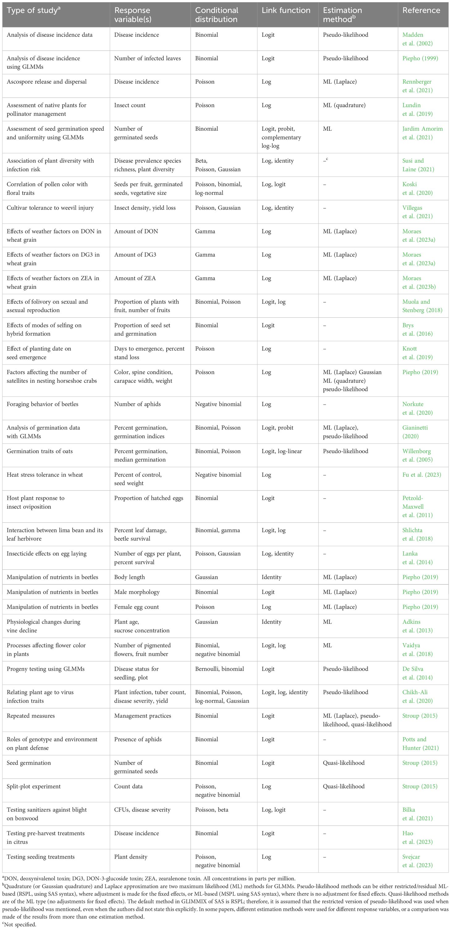
Table 4 Summary of some applications of generalized linear mixed models in the analysis of data from designed experiments in agricultural and horticultural systems.
Binomial, NB, gamma, and Poisson were the most commonly used conditional distributions in these studies, while beta (Bilka et al., 2021; Susi and Laine, 2021) and Bernoulli (a special case of binomial with n = 1) (De Silva et al., 2014) were less frequently used. The link functions specified in the models in these studies were logit, log, probit, complementary log–log, and identity (i.e., no transformation of the mean). While several papers provided details on how model fitting was conducted and specified the estimation method [ML (quadrature or Laplace), PL, or quasi-likelihood)] used, other papers did not provide details of the estimation method used. We made no attempt to establish whether the model, the link function, or the estimation method specified in these studies was appropriately specified by the authors to match the data and the aims of individual studies. Furthermore, we did not evaluate whether the authors interpreted the results appropriately. This summary shows that the application of GLMMs in the above disciplines is diverse and is used to address hypotheses in a wide range of experimental conditions. We expect this to grow as researchers appreciate the clear argument of matching the model to the data (for a given experimental and treatment design) when using GLMMs for analysis.
11 Summary and conclusions
There are several reasons to use GLMMs for the analysis of non-normal data, some of which were discussed in this paper, with many more details in several references (Littell et al., 2006; Bolker et al., 2009; Zuur et al., 2009; Gbur et al., 2012; Stroup, 2013; Brown and Prescott, 2015; Stroup et al., 2018; Gianinetti, 2020; Li et al., 2023; Ruíz et al., 2015, 2023). Perhaps the biggest argument is that one is better off matching the model to the data with a GLMM rather than changing (i.e., transforming) the data to match the model, as with a LMM (Gbur et al., 2012; Stroup, 2013). With some contemporary software, it is deceptively easy now to switch from normality-based LMMs to non-normality-based GLMMs. For instance, this simple model statement in the GLIMMIX procedure of SAS can be used to fit a LMM to the response variable y for a RCBD (as in our example):
(Random effects, such as blocks, are given in separate statements, and the identification of explanatory variables as factors is done in a separate statement). Using the same procedure, a conditional–binomial GLMM with a logit link function can be fitted to the same data with only one minor change to the model statement:
with all other statements (not shown here) being the same. The procedure automatically identifies this as a conditional binomial with logit link when the left-hand side of the equation is given as the ratio of a response variable to the number of individuals (i.e., y/n). Of course, the distribution (dist=) and link (link=) can be explicitly specified as options with this procedure (Gbur et al., 2012; Brown and Prescott, 2015; Ruiz et al., 2023), allowing for many different conditional distributions and links. However, this simple switch would be fitting the naive model A (Equation 13) to the RCBD data (assuming the block random effect was also specified). This is because, with an LMM, a residual is always estimated to account for the plot variability (in a field study) after accounting for other sources of variability, but is not estimated with a conditional binomial (or conditional Poisson). The variance is always nπ(1 − π) for a conditional binomial and always μ for the conditional Poisson. In separate statements for random effects, the block × treatment random term (vij) would need to be added to fit model B (Equation 16), or the conditional distribution to be changed from binomial to a quasi-binomial likelihood with the ϕ overdispersion parameter to account for overdispersion (model C; Equation 17). Alternatively, a more complex conditional distribution could be used, such as the beta-binomial (but not with the GLIMMIX procedure).
The important point here is that one should never lose sight of the experimental design when analyzing data (Piepho et al., 2003; Bello et al., 2004, 2016), as well as how to account for the relevant aspects of the design (fixed effects, random effects, and correlations) in the model (e.g., right-hand side of the equation for η, plus distributions for random effects) for any selected conditional distribution, whether using LMMs or GLMMs. Readers should consult Stroup (2013, 2015) for a more thorough discussion on this topic. Adding terms to a GLMM (or modifying conditional distributions) may be needed to account for the sources of variability that are automatically accounted for with LMMs.
In this paper, we emphasized the switch from LMM to GLMM, with the assumption that the reader is more familiar with LMMs. We mostly restricted our attention to one type of response variable [discrete observations (counts) that can be represented as proportions or percentages] and one experimental design, namely, a RCBD. This approach was chosen to show the similarities and differences between LMMs and GLMMs, focusing on one small dataset. The differences in the results between LMMs and GLMMs will be greater in other datasets with larger random effect variances and when some of the πi values are closer to 0 or 1 for some treatments (Stroup, 2013). The differences between LMMs and GLMMs carry through to more complex experimental and treatment designs (Gbur et al., 2012; Ruíz et al., 2023). Issues in data analysis that are mostly well resolved for LMMs remain debatable with GLMMs. For instance, appropriate model fitting (estimation) can be controversial for GLMMs (Stroup and Claassen, 2020). In fact, some models, such as those involving a quasi-likelihood (e.g., models with an overdispersion parameter, ϕ), can only be fitted using certain estimation methods (either pseudo-likelihood or quasi-likelihood). For other models, investigators have choices for model fitting, and the best choice depends on the circumstances, as presented above. Despite earlier criticisms, linearization methods, particularly the restricted versions such as RSPL (analogous to REML for LMMs), have been shown recently to often be the best choice for model fitting, especially for discrete data and the small sample sizes typically used in field studies in agriculture (Stroup and Claassen, 2020). Integral approximations of the marginal likelihood (such as quadrature and Laplace) do have advantages when there are reasonably large numbers of replicates, especially when one is interested in comparing the goodness of fit of different models through differences in the log-likelihood or have specific interest in the variances and covariances.
A key distinction of LMMs and GLMMs is the notion of conditional versus marginal means (Stroup, 2013). Conditional and marginal means are the same for normality-based LMMs, but are different, in general, for GLMMs. The magnitude of the random effect variances has a large influence on the magnitude of the difference between the conditional and marginal means. We agree with Stroup (2013, 2015) and Stroup et al. (2018) that most researchers would find the conditional means as being more meaningful and of primary interest, thus emphasizing the importance of conditional models in a GLMM-based analysis. The use of a conditional model, however, still allows for broad or narrow inference when testing hypotheses or calculating the confidence intervals for parameters or parameter differences. Inference space (broad vs. narrow) has to do with whether inference is over the entire population of random effects (say, all possible blocks, locations, etc.) or only for the specific random effect levels in the study. Littell et al. (2006) and Stroup (2013) should be consulted for more detail on this topic.
Author contributions
LM: Conceptualization, Formal analysis, Writing – original draft, Writing – review & editing. PO: Conceptualization, Data curation, Writing – review & editing.
Funding
The author(s) declare that no financial support was received for the research, authorship, and/or publication of this article.
Conflict of interest
The authors declare that the research was conducted in the absence of any commercial or financial relationships that could be construed as a potential conflict of interest.
The author(s) declared that they were an editorial board member of Frontiers, at the time of submission. This had no impact on the peer review process and the final decision.
Publisher’s note
All claims expressed in this article are solely those of the authors and do not necessarily represent those of their affiliated organizations, or those of the publisher, the editors and the reviewers. Any product that may be evaluated in this article, or claim that may be made by its manufacturer, is not guaranteed or endorsed by the publisher.
Supplementary material
The Supplementary Material for this article can be found online at: https://www.frontiersin.org/articles/10.3389/fhort.2024.1423462/full#supplementary-material
References
Adkins S., McCollum T. G., Albano J. P., Kousik C. S., Baker C. A., Webster C. G., et al. (2013). Physiological effects of Squash vein yellowing virus infection on watermelon. Plant Dis. 97, 1137–1148. doi: 10.1094/PDIS-01-13-0075-RE
Albert A., Anderson J. A. (1984). On the existence of maximum likelihood estimates in logistic regression models. Biometrika 71, 1–10. doi: 10.1093/biomet/71.1.1
Basak I., Balakrishnan N. (2012). Estimation for the three-parameter gamma distribution based on progressively censored data. Stat. Methodol. 9, 305–319. doi: 10.1016/j.stamet.2011.08.005
Bello N. M., Kramer M., Tempelman R. J., Stroup W. W., St-Pierre N. R., Craig B. A., et al. (2016). On recognizing the proper experimental unit in animal studies in the dairy sciences. J. Dairy Sci. 99, 8871–8879. doi: 10.3168/jds.2016-11516
Bilka R., Copes W., Baysal-Gurel F. (2021). Comparative performance of sanitizers in managing plant-to-plant transfer and postharvest infection of Calonectria pseudonaviculata and Pseudonectria foliicola on boxwood. Plant Dis. 105, 2809–2821. doi: 10.1094/PDIS-03-21-0481-RE
Bolker B. M., Brooks M. E., Clark C. J., Geange S. W., Poulsen J. R., Stevens M. H., et al. (2009). Generalized linear mixed models: a practical guide for ecology and evolution. Trends Ecol. Evol. 24, 127–135. doi: 10.1016/j.tree.2008.10.008
Bolker B., Piaskowski J., Tanaka E., Alday P., Viechtbauer W. (2022) CRAN Task View: Mixed, Multilevel, and Hierarchical Models in R. Available online at: https://CRAN.R-project.org/view=MixedModels.
Breslow N. E., Clayton D. G. (1993). Approximate inference in generalized linear mixed models. J. Amer. Stat. Assoc. 88, 9–25. doi: 10.1080/01621459.1993.10594284
Brown H., Prescott R. (2015). Applied Mixed Models in Medicine (Chichester, UK: Third Edition. John Wiley & Sons).
Brys R., van Cauwenberghe J., Jacquemyn H. (2016). The importance of autonomous selfing in preventing hybridization in three closely related plant species. J. Ecol. 104, 601–610. doi: 10.1111/1365-2745.12524
Chikh-Ali M., Tran L. T., Price W. J., Karasev A. V. (2020). Effects of the age-related resistance to Potato virus Y in potato on the systemic spread of the virus, incidence of the potato tuber necrotic ringspot disease, tuber yield, and translocation rates into progeny tubers. Plant Dis. 104, 269–275. doi: 10.1094/PDIS-06-19-1201-RE
Claassen E. A. (2014). A Reduced Bias Method of Estimating Variance Components in Generalized Linear Mixed Models (Digital Commons, University of Nebraska-Lincoln). Available at: https://digitalcommons.unl.edu/statisticsdiss/13/. Ph.D. Dissertation, Lincoln, Nebraska.
Clark R. G., Blanchard W., Hui F. K. C., Tian R., Woods H. (2023). Dealing with complete separation and quasi-complete separation in logistic regression for linguistic data. Res. Methods Appl. Linguistics 2, 1000444. doi: 10.1016/j.rmal.2023.100044
Cohen A. C. Jr. (1960). Estimating the parameter in a conditional Poisson distribution. Biometrics 16, 203–211. doi: 10.2307/2527552
Couton J., Stroup W. (2013). “On the small sample behavior of generalized linear mixed models with complex experiments,” in Conference on Applied Statistics in Agriculture (Kansas State University, Manhattan, KS). doi: 10.4148/2475–7772.1012
De Silva N. H., Gea L., Lowe R. (2014). Genetic analysis of resistance to Pseudomonas syringae pv. actinidiae (Psa) in a kiwifruit progeny test: An application of generalised linear mixed models (GLMMs) Vol. 3 (SpringerPlus), 547. doi: 10.1186/2193-1801-3-547
Diaz-Ramirez L. G., Jing B., Covinsky K. E., Boscardin W. J. (2020). “Mixed-effects models and complex survey data with the GLIMMIX procedure,” in SAS Global Forum, (SAS Inc., Cary, NC) 4937–2020. Available at: https://support.sas.com/resources/papers/proceedings20/4937–2020.pdf.
Dixon P. (2016). Conference on Applied Statistics in Agriculture. Kansas State University, Manhattan, KS. doi: 10.4148/2475–7772.1474
Eisenhart C. (1947). The assumptions underlying the analysis of variance. Biometrics 3, 1–21. doi: 10.2307/3001534
Firth D. (1993). Bias reduction of maximum likelihood estimates. Biometrika 80, 27–38. doi: 10.1093/biomet/80.1.27
Fisher R. A. (1918). The correlation between relatives on the supposition of Mendelian inheritance. Trans. R. Soc Edinburgh 52, 399–433. doi: 10.1017/S0080456800012163
Fu J., Bowden R. L., Jagadish S. V. K., Prasad P. V. V. (2023). Genetic variation for terminal heat stress tolerance in winter wheat. Front. Plant Sci. 14. doi: 10.3389/fpls.2023.1132108
Gbur E. E., Stroup W. W., McCarter K. S., Durham S., Young L. J., Christman M., et al. (2012). Analysis of Generalized Linear Mixed Models in the Agricultural and Natural Resources Sciences (Madison, WI, USA: American Society of Agronomy, Soil Science Society of America, Crop Science of America, Inc). doi: 10.2134/2012.generalized-linear-mixed-models
Gianinetti A. (2020). Basic features of the analysis of germination data with generalized linear mixed models. Data 5, 1–42. doi: 10.3390/data5010006
Hao W., Förster H., Belisle R. J., Adaskaveg J. E. (2023). New preharvest treatments and strategies in managing Phytophthora brown rot of citrus in California. Plant Dis. 107, 2081–2087. doi: 10.1094/PDIS-08-22-1917-RE
Harville D. A. (1977). Maximum-likelihood approaches to variance component estimation and to related problems. J. Amer. Stat. Assoc. 72, 320–340. doi: 10.1080/01621459.1977.10480998
Heinze G., Schemper M. (2002). A solution to the problem of separation in logistic regression. Stat. Med. 21, 2409–2419. doi: 10.1002/sim.1047
Henderson C. R. (1953). Estimation of variance and covariance components. Biometrics 9, 226–252. doi: 10.2307/3001853
Henderson C. R. (1984). Applications of Linear Models in Animal Breeding (Canada: University of Guelph).
Hughes G., Madden L. V. (1995). Some methods allowing for aggregated patterns of disease incidence in the analysis of data from designed experiments. Plant Pathol. 44, 927–943. doi: 10.1111/j.1365-3059.1995.tb02651.x
Hughes G., McRoberts N., Madden L. V. (2004). Daamen’s incidence-severity relationship revisited. Eur. J. Plant Pathol. 110, 759–761. doi: 10.1023/B:EJPP.0000041550.29236.d1
Hughes G., Munkvold G. P., Samita S. (1998). Application of the logistic-normal-binomial distribution to the analysis of Eutypa dieback disease incidence. Int. J. Pest Manage. 44, 35–42. doi: 10.1080/096708798228509
Jardim Amorim D., Pereira dos Santos A. R., Nunes da Piedade G., Quelvia de Faria R., Amaral da Silva E. A., Pereira Sartori M. M. (2021). The use of the generalized linear model to assess the speed and uniformity of germination of corn and soybean seeds. Agronomy 11, 588. doi: 10.3390/agronomy11030588
Joe H. (2008). Accuracy of Laplace approximation for discrete response mixed models. Comput. Stat. Data Anal. 52, 5066–5074. doi: 10.1016/j.csda.2008.05.002
Knott C., Herbek J., James J. (2019). Early planting dates maximize soybean yield in Kentucky. Crop Forage Turfgrass Manage. 5, 180085. doi: 10.2134/cftm2018.10.0085
Koski M. H., Berardi A. E., Galloway L. F. (2020). Pollen colour morphs take different paths to fitness. J. Evol. Biol. 33, 388–400. doi: 10.1111/jeb.13599
Kramer M. H., Paparozzi E. T., Stroup W. W. (2016). Statistics in a horticultural journal: Problems and solutions. J. Amer. Soc Hortic. Sci. 141, 400–406. doi: 10.21273/JASHS03747-16
Kriss A. B., Paul P. A., Madden L. V. (2012). Characterizing heterogeneity of disease incidence in a spatial hierarchy: A case study from a decade of observations of Fusarium head blight of wheat. Phytopathology 102, 867–877. doi: 10.1094/PHYTO-11-11-0323
Laird N. M., Ware J. H. (1982). Random-effects models for longitudinal data. Biometrics 38, 963–974. doi: 10.2307/2529876
Lambert D. (1992). Zero-inflated Poisson regression, with an application to defects in manufacturing. Technometrics 34, 1–14. doi: 10.2307/1269547
Lanka S. K., Stout M. J., Beuzelin J. M., Ottea J. A. (2014). Activity of chlorantraniliprole and thiamethoxam seed treatments on life stages of the rice water weevil as affected by the distribution of insecticides in rice plants. Pest Manage. Sci. 70, 338–344. doi: 10.1002/ps.3570
Lee Y., Nelder J. A. (1996). Hierarchical generalized linear models. J. R. Stat. Soc B 58, 619–656. doi: 10.1111/j.2517-6161.1996.tb02105.x
Lee Y., Nelder J. A., Pawitan Y. (2006). Generalized Linear Models with Random Effects: Unified Analysis via H-Likelihood. 2nd ed. (Boca Raton, FL: Chapman and Hall). doi: 10.1201/9781420011340
Li H., Luo W., Back E., Thompson C. G., Lam K. H. (2023). Multilevel modeling in single-case studies with count and proportion data: A demonstration and evaluation. Psychol. Methods. doi: 10.1037/met0000607
Liang K.-Y., Zeger S. L. (1986). Longitudinal data analysis using generalized linear models. Biometrika 73, 13–22. doi: 10.1093/biomet/73.1.13
Littell R. C., Milliken G. A., Stroup W. W., Wolfinger R. D., Schabenberger O. (2006). SAS for Mixed Models. 2nd ed. (Cary, NC: SAS Press).
Lundin O., Ward K. L., Williams N. M. (2019). Identifying native plants for coordinated habitat management of arthropod pollinators, herbivores and natural enemies. J. Appl. Ecol. 56, 665–676. doi: 10.1111/1365-2664.13304
Madden L. V., Hughes G. (1995). Plant disease incidence: distributions, heterogeneity, and temporal analysis. Annu. Rev. Phytopathol. 33, 529–564. doi: 10.1146/annurev.py.33.090195.002525
Madden L. V., Hughes G., Moraes W. B., Xu X.-M., Turechek W. W. (2018). Twenty-five years of the binary power law for characterizing heterogeneity of disease incidence. Phytopathology 108, 656–680. doi: 10.1094/PHYTO-07-17-0234-RVW
Madden L. V., Hughes G., van den Bosch F. (2007). The Study of Plant Disease Epidemics (American Phytopathological Society, St. Paul, MN: APS Press).
Madden L. V., Paul P. A. (2009). Assessing heterogeneity in the relationship between wheat yield and Fusarium head blight intensity using random-coefficient mixed models. Phytopathology 99, 850–860. doi: 10.1094/PHYTO-99-7-0850
Madden L. V., Turechek W. W., Nita M. (2002). Evaluation of generalized linear mixed models for analyzing disease incidence data obtained in designed experiments. Plant Dis. 86, 316–325. doi: 10.1094/PDIS.2002.86.3.316
Malik W. A., Marco-Llorca C., Berendzen K., Piepho H.-P. (2020). Choice of link and variance function for generalized linear mixed models: a case study with binomial response in proteomics. Commun. Stat. Theory Methods 49, 4313–4332. doi: 10.1080/03610926.2019.1599021
McCullagh P., Nelder J. A. (1989). Generalized Linear Models. 2nd ed. (Chapman & Hall, New York). doi: 10.1007/978-1-4899-3242-6
McCulloch C. E., Neuhaus J. M. (2011). Misspecifying the shape of a random effects distribution: Why getting it wrong may not matter. Stat. Sci. 26, 388–402. doi: 10.1214/11-STS361
McCulloch C. E., Searle S. R. (2001). Generalized, Linear, and Mixed Models. (New York: John Wiley & Sons).
Milliken G. A., Johnson D. E. (2009). Analysis of Messy Data, Volume 1: Designed Experiments. 2nd ed. (Boca Raton, FL: CRC Press). doi: 10.1201/EBK1584883340
Moraes W. B., Madden L. V., Baik B.-K., Gillespie J., Paul P. A. (2023a). Environment, grain development, and harvesting strategy effects on zearolenone contamination of grain from Fusarium head blight-affected wheat spikes. Phytopathology 113, 225–238. doi: 10.1094/PHYTO-05-22-0190-R
Moraes W. B., Madden L. V., Baik B., Gillespie J., Paul P. A. (2023b). Environmental conditions after Fusarium head blight visual symptom development affect contamination of wheat grain with deoxynivalenol and deoxynivalenol-3Dglucoside. Phytopathology 113, 206–224. doi: 10.1094/PHYTO-06-22-0199-R
Moraes W. B., Madden L. V., Paul P. A. (2022). Efficacy of genetic resistance and fungicide application against Fusarium head blight and mycotoxins in wheat under persistent pre-and postanthesis moisture. Plant Dis. 106, 2839–2855. doi: 10.1094/PDIS-02-22-0263-RE
Morel J. G., Neerchal N. K. (2010). “Extra variation models,” in Encyclopedia of Biopharmaceutical Statistics, 3rd ed. Ed Chow S.-C. (Informa Healthcare, London).
Muola A., Stenberg J. A. (2018). Folivory has long-term effects on sexual but not on asexual reproduction in woodland strawberry. Ecol. Evol. 8, 12250–12259. doi: 10.1002/ece3.4687
Norkute M., Olsson U., Ninkovic V. (2020). Aphids-induced plant volatiles affect diel foraging behavior of a ladybird beetle. Coccinella septempunctata. Insect Sci. 27, 1266–1275. doi: 10.1111/1744-7917.12734
Paul P. A., El-Allaf S. M., Lipps P. E., Madden L. V. (2005). Relationships between incidence and severity of Fusarium head blight on winter wheat in Ohio. Phytopathology 95, 1049–1060. doi: 10.1094/PHYTO-95-1049
Paul P. A., Salgado J. D., Bergstrom G. C., Bradley C., Byamukama E., Byrne A. M., et al. (2019). Integrated effects of genetic resistance and prothioconazole + tebuconazole application timing on Fusarium head blight in wheat. Plant Dis. 103, 223–237. doi: 10.1094/PDIS-04-18-0565-RE
Petzold-Maxwell J., Wong S., Arellano C., Gould F. (2011). Host plant direct defence against eggs of its specialist herbivore, Heliothis subflexa. Ecol. Entomol. 36, 700–708. doi: 10.1111/j.1365-2311.2011.01315.x
Piepho H. P. (1999). Analysing disease incidence data from designed experiments by generalized linear mixed models. Plant Pathol. 48, 668–674. doi: 10.1046/j.1365-3059.1999.00383.x
Piepho H. P. (2003). The folded exponential transformation for proportions. J. R. Stat. Soc.: Ser. D 52, 575–589. doi: 10.1046/j.0039-0526.2003.00509.x
Piepho H. P. (2009). Data transformation in statistical analysis of field trials with changing treatment variance. Agron. J. 101, 865–869. doi: 10.2134/agronj2008.0226x
Piepho H. P. (2019). A coefficient of determination (R2) for generalized linear mixed models. Biom. J. 61, 860–872. doi: 10.1002/bimj.201800270
Piepho H. P. (2023). An adjusted coefficient of determination (R2) for generalized linear mixed models in one go. Biom. J. 65, 2200290. doi: 10.1002/bimj.202200290
Piepho H. P., Büchse A., Emrich K. (2003). A hitchhiker’s guide to mixed models for randomized experiments. J. Agron. Crop Sci. 189, 310–322. doi: 10.1046/j.1439-037X.2003.00049.x
Piepho H. P., Büchse A., Richter C. (2004). A mixed modelling approach for randomized experiments with repeated measures. J. Agron. Crop Sci. 190, 230–247. doi: 10.1111/j.1439-037X.2004.00097.x
Piepho H. P., Madden L. V. (2022). How to observe the principle of concurrent control in an arm-based meta-analysis using SAS procedures GLIMMIX and BGLIMM. Res. Syn. Meth. 13, 821–828. doi: 10.1002/jrsm.1576
Piepho H. P., Madden L. V., Roger J., Payne R., Williams E. R. (2018). Estimating the variance for heterogeneity in arm-based network meta-analysis. Pharm. Stat. 17, 264–277. doi: 10.1002/pst.1857
Potts A. S., Hunter M. D. (2021). Unraveling the roles of genotype and environment in the expression of plant defense phenotypes. Ecol. Evol. 11, 8542–8561. doi: 10.1002/ece3.7639
Rao C. R. (1972). Estimation of variance and covariance components in linear models. J. Amer. Stat. Assoc. 67, 112–115. doi: 10.1080/01621459.1972.10481212
Rennberger G., Turechek W. W., Keinath A. P. (2021). Dynamics of the ascospore dispersal of Stagonosporopsis citrulli, a causal agent of gummy stem blight of cucurbits. Plant Pathol. 70, 1908–1919. doi: 10.1111/ppa.13424
Ruíz J. S., López O. A. M., Ramírez G. H., Hiriat J. C. (2023). Generalized Linear Mixed Models with Applications in Agriculture and Biology. (Switzerland: Springer). doi: 10.1007/978-3-031-32800-8
Schabenberger O., Pierce F. J. (2002). Contemporary Statistical Models for the Plant and Soil Sciences (Boca Raton, FL: CRC Press). doi: 10.1201/9781420040197
Schielzeth H., Dingemanse N. J., Nakagawa S., Westneat D. F., Allegue H., Teplitsky C., et al. (2020). Robustness of linear mixed-effects models to violations of distributional assumptions. Methods Ecol. Evol. 11, 1141–1152. doi: 10.1111/2041-210X.13434
Shlichta J. G., Cuny M. A. C., Hernandez-Cumplido J., Traine J., Benrey B. (2018). Contrasting consequences of plant domestication for the chemical defenses of leaves and seeds in lima bean plants. Basic Appl. Ecol. 31, 10–20. doi: 10.1016/j.baae.2018.05.012
Steel R. G. D., Torrie J. H. (1960). Principles and Procedures of Statistics (New York: McGraw-Hill Book Company). With special Reference to the Biological Sciences.).
Stroup W. W. (2013). Generalized Linear Mixed Models: Modern Concepts, Methods and Applications (Boca Raton, FL: CRC Press).
Stroup W. W. (2015). Rethinking the analysis of non-normal data in plant and soil science. Agron. J. 107, 811–827. doi: 10.2134/agronj2013.0342
Stroup W. W. (2021). Bayesian analysis of GLMMs using PROC BGLMM (SAS Global Forum Paper, SAS Inc., Cary, NC), 1146–2021.
Stroup W., Claassen E. (2020). Pseudo-likelihood or quadrature? What we thought we knew, what we think we know, and what we are still trying to figure out. J. Agric. Biol. Environ. Stat. 25, 639–656. doi: 10.1007/s13253-020-00402-6
Stroup W. W., Milliken G. A., Claassen E. A., Wolfinger R. D. (2018). SAS for Mixed Models: Introduction and Basic Applications. (Cary, NC: SAS Press).
Susi H., Laine A. L. (2021). Agricultural land use disrupts biodiversity mediation of virus infections in wild plant populations. New Phytol. 230, 2447–2458. doi: 10.1111/nph.17156
Svejcar L. N., Kerby J. D., Svejcar T. J., Mackey B., Boyd C. S., Baughman O. W., et al. (2023). Plant recruitment in drylands varies by site, year, and seeding technique. Restor. Ecol. 31, e13750. doi: 10.1111/rec.13750
Turechek W. W., Madden L. V. (1999). Spatial pattern analysis of strawberry leaf blight in perennial production systems. Phytopathology 89, 421–433. doi: 10.1094/PHYTO.1999.89.5.421
Turechek W. W., Madden L. V. (2003). A generalized linear modeling approach for characterizing disease incidence in a spatial hierarchy. Phytopathology 93, 458–466. doi: 10.1094/PHYTO.2003.93.4.458
Vaidya P., McDurmon A., Mattoon E., Keefe M., Carley L., Lee C., et al. (2018). Ecological causes and consequences of flower color polymorphism in a self-pollinating plant (Boechera stricta). New Phytol. 218, 380–392. doi: 10.1111/nph.14998
Villegas J. M., Wilson B. E., Way M. O., Gore J., Stout M. J. (2021). Tolerance to rice water weevil, Lissorhoptrus oryzophilus Kuschel (Coleoptera: Curculionidae), infestations among hybrid and inbred rice cultivars in the Southern U.S. Crop Prot. 139, 105368. doi: 10.1016/j.cropro.2020.105368
Willenborg C. J., Wildeman J. C., Miller A. K., Rossnagel B. G., Shirtliffe S. J. (2005). Oat germination characteristics differ among genotypes, seed sizes, and osmotic potentials. Crop Sci. 45, 2023–2029. doi: 10.2135/cropsci2004.0722
Wolfinger R. D., Kass R. E. (2000). Nonconjugate Bayesian analysis of variance component models. Biometrics 56, 768–774. doi: 10.1111/j.0006-341X.2000.00768.x
Wolfinger R. D., O’Connell M. (1993). Generalized linear mixed models: A pseudo-likelihood approach. J. Stat. Comput. Simul. 4, 233–243. doi: 10.1080/00949659308811554
Xie L., Madden L. V. (2014). %HPGLIMMIX, a high performance SAS macro for GLMM estimation. J. Stat. Software 58, 1–25. doi: 10.18637/jss.v058.i08
Yates F. (1940). The recovery of interblock information in balanced incomplete block designs. Ann. Eugen. 10, 317–325.
Zuur A. F., Ieno E. N., Walker N. J., Saveliev A. A., Smith G. M. (2009). Mixed Effects Models and Extensions in Ecology with R. (New York: Springer). doi: 10.1007/978-0-387-87458-6
Keywords: binomial, conditional distribution, fixed effects, integral approximation, marginal distribution, pseudo-likelihood, random effects, quasi-likelihood
Citation: Madden LV and Ojiambo PS (2024) The value of generalized linear mixed models for data analysis in the plant sciences. Front. Hortic. 3:1423462. doi: 10.3389/fhort.2024.1423462
Received: 25 April 2024; Accepted: 04 June 2024;
Published: 25 June 2024.
Edited by:
Xiangming Xu, National Institute of Agricultural Botany (NIAB), United KingdomReviewed by:
Kuo-Szu Chiang, National Chung Hsing University, TaiwanHannah M. Rivedal, Agricultural Research Service (USDA), United States
Copyright © 2024 Madden and Ojiambo. This is an open-access article distributed under the terms of the Creative Commons Attribution License (CC BY). The use, distribution or reproduction in other forums is permitted, provided the original author(s) and the copyright owner(s) are credited and that the original publication in this journal is cited, in accordance with accepted academic practice. No use, distribution or reproduction is permitted which does not comply with these terms.
*Correspondence: Laurence V. Madden, bWFkZGVuLjFAb3N1LmVkdQ==