Accurate leaf area index estimation for Eucalyptus grandis using machine learning method with GF-6 WFV—A case study for Huangmian town, China

Spectral and texture features play important roles in plantation leaf area index (LAI) estimation, and their combination may enhance LAI inversion accuracy. Furthermore, research on the impact of different machine learning (ML) models on their hyperparameter combinations and splitting ratios remains challenging. In our study, experiments based on spectral and textural features of GF-6 WFV data were conducted on Eucalyptus grandis plantation forests in Huangmian Town, Guangxi, China. ML methods such as multiple stepwise regression (MSR), random forest (RF), back-propagation neural network (BPNN), and support vector regression (SVR) were mainly utilized to perform model hyper-parameter tuning and split-ratio analysis in order to estimate the LAI. The results of the study showed that spectral and gray level co-occurrence matrix (GLCM) texture features were very sensitive to changes in Eucalyptus grandis LAI. The accuracy of combining the two was 10% higher than when they were not combined. Furthermore, it was found that the nonlinear methods (RF, BPNN, and SVR) outperformed the linear method (MSR), with the average $R_{\text{max}}^2$ of the nonlinear model being 26% higher than that of the linear model, and the RMSE value being 29% lower than that of the linear model. In addition, by analyzing different combinations of features, model hyperparameter fine-tuning, and splitting ratios in the nonlinear model, it was found that the splitting ratios of different combinations of model hyperparameters have a great impact on the accuracy of the model. A total of 12 out of 21 data sets showed high accuracy and stability at a split ratio of 8.5:1.5 (ratio of 0.85), with the best-performing RF model differing from the lowest by 91% for $R_{\text{max}}^2$ and 39% for $R_{std}^2$ . Combining spectral and texture features provides highly accurate inversion data. Model hyper-parameter fine-tuning and segmental scale tuning can facilitate the application of inversion data to fully utilize the optimal performance of the ML model.

1 Introduction

Eucalyptus is one of the globally important economic tree species, primarily used for pulp production, playing an indispensable role in the paper and timber industries (Myburg et al., 2014). Eucalyptus grandis stands out among Eucalyptus species for being extensively cultivated in tropical and subtropical areas, largely because of its quick growth and high-quality material (Ouyang et al., 2018). It adapts well to high-humidity environments and is commonly used in forestry production in wetlands and coastal areas. E. grandis’s growth characteristics directly affect the leaf area index (LAI), which is an important parameter for assessing forest productivity and ecological processes (Jin et al., 2015). Due to the significant differences in LAI magnitude among different Eucalyptus species, it is crucial to specify the tree species for LAI estimation in the study. This study focuses on E. grandis, a tree species whose rapid growth and high LAI make it an important target for LAI inversion by remote sensing techniques (Tesfamichael et al., 2018).

Traditional field-based LAI measurements require a significant amount of manpower and time, with limited scalability, making it difficult for widespread application (Wang et al., 2022). In recent years, the rapid development of remote sensing technology has provided a powerful tool for large-scale, high-frequency LAI monitoring. The Sentinel satellite series, the Landsat satellite series, and the Chinese high-resolution remote sensing satellite series have been widely applied in various fields and proven to be reliable data sources for vegetation monitoring and LAI estimation (Aparicio et al., 2002; Yang et al., 2022a; Yang et al., 2015). These satellites provide observations in multiple spectral bands, including visible light and infrared, which are closely related to the physiological characteristics of vegetation and can be used to infer vegetation LAI (Padalia et al., 2020). Additionally, there is a correlation between vegetation indices (VIs) calculated from remote sensing data and LAI. By analyzing this correlation, a better understanding of vegetation growth status and spatial distribution characteristics can be achieved, providing important information for vegetation monitoring, ecological research, and resource management (Ma et al., 2021). However, these spectral characteristics are susceptible to the mixed effects of different land cover types within remote sensing pixels. Particularly in tall tree species like Eucalyptus, single spectral features may not comprehensively represent their LAI variations (Tuominen and Pekkarinen, 2005).

In LAI inversion, texture features also play a crucial role (Zhang et al., 2021). These features quantify the spatial distribution and variation patterns of surface remote sensing images through texture analysis methods (Iqbal et al., 2021). Among them, the spatial distribution of surface cover is a critical component of texture features, reflecting the spatial distribution patterns of vegetation and non-vegetation areas in remote sensing images (Madonsela et al., 2017). This is crucial for LAI inversion because the density and spatial organization of vegetation directly impact the accuracy and precision of LAI estimation. Additionally, the regular planting pattern of Eucalyptus plantations leads to distinct texture features during the seedling stage, while the texture information weakens in mature forests (Zhou et al., 2013), making texture features a key factor in inverting Eucalyptus LAI (Couteron et al., 2005). This highlights the significant role of texture features in improving the accuracy of LAI estimation and understanding spatial distribution characteristics. On one hand, there is currently a lack of research on texture features specific to Eucalyptus, and it remains unclear how specific texture features affect the accuracy and precision of Eucalyptus LAI estimation. On the other hand, despite the widely recognized role of texture features in LAI inversion, how to most effectively integrate these features to enhance the performance of inversion models remains an unresolved issue. Therefore, further research is needed to explore the relationship between Eucalyptus LAI and texture features, revealing their potential mechanisms and patterns.

Applying machine learning (ML) methods is an important approach to establish the relationship between remote sensing features and forest growth parameters (Wu et al., 2023b). In ML, regression models can be classified into two main categories: linear and nonlinear (Ma et al., 2022; Matese and Di Gennaro, 2021). Linear models assume a linear relationship between the dependent and independent variables. Compared to linear regression models, nonlinear regression models are usually more complicated and request more parameter adjustments (Krupnik et al., 2015). Nonlinear models outperform linear models because they can more accurately capture the complex nonlinear relationships between measured variables and predicted variables (Aworka et al., 2022).

To enhance the accuracy of ML in LAI inversion, it is crucial to consider two important issues: model parameter optimization and the proportion of samples allocated for training and validation. Selecting appropriate parameters ensures that the model accurately captures the complex relationships between vegetation features and environmental factors, thereby improving the accuracy of LAI predictions (Andrade et al., 2020). Moreover, choosing the right split ratio balances model training and evaluation, mitigating issues such as overfitting or underfitting (Roshan et al., 2022). For example, Weerts et al. (2020) pointed out that selecting different parameter settings can affect the performance of the model. Probst et al. (2019) conducted large-scale benchmark testing studies on 38 datasets and six common hyperparameters based on ML models, finding that selecting appropriate hyperparameters can improve the model’s accuracy. Yang and Shami (2020) noted that fine-tuning of the hyperparameters of ML models is essential in order to address the issue of their effective utilization. This tuning ensures that the model is optimized so that it performs well on the particular dataset to be analyzed. Nguyen et al. (2021) tested three ML models with different split ratios (i.e., 10/90, 20/80, 30/70, 40/60, 50/50, 60/40, 70/30, 80/20, and 90/10), finding that the predictive ability of the models is greatly influenced by the ratio of the training set to the test set, with the 70/30 ratio model performing the best.

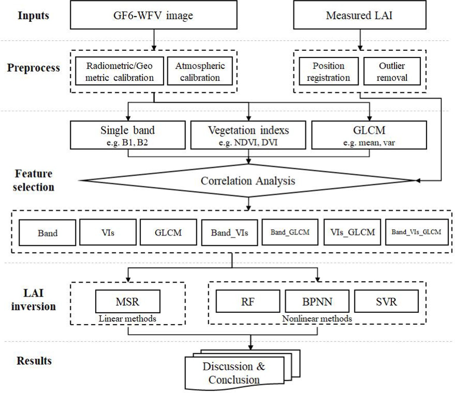
This study aims to invert E. grandis LAI using spectral and texture features of GF-6 WFV, for which three hypotheses are formulated: (1) E. grandis LAI can be accurately inverted by the spectral and texture features of GF-6 WFV. (2) The inclusion of texture features significantly improves the inversion accuracy. (3) The non-linear machine learning model outperforms the linear model and better captures the complex relationship between LAI and the features of satellite data. To test the hypothesis, the relationship between LAI and the spectral and textural properties of GF-6 WFVs was analyzed by linear and nonlinear models, grid search was used to optimize the hyperparameters, and the ratio of training set to validation set was debugged. Finalization of models to support E. grandis growth monitoring and yield prediction. In addition, we developed a user-friendly machine-learning framework that includes parameter combination analysis, model parameter search, optimal model identification, and training (Figure 1).¹

Figure 1

Figure 1. Technology road map.

2 Materials and methods

2.1 Study area

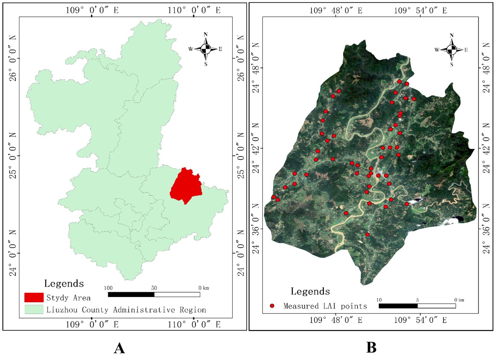
Huangmian Town is located at the eastern edge of Luzhai County, Guangxi Province, between 109°28′-110°12′E longitude and 24°14′-24°50′N latitude, as shown in Figure 2A. The altitude range of the town is 83 ~ 826 m. It is located in the transition zone from the southern subtropical zone to the central subtropical zone, with a mild climate and an average annual temperature of about 20°C. The highest temperature in summer is 37°C and the lowest temperature in winter is 0°C. Sunlight is relatively abundant and rainfall is plentiful, with rainfall mainly concentrated from April to July with an average annual precipitation of about 1,300 mm. The average annual sunshine hours is about 1,600 and the frost-free period is more than 320 days, which is suitable for the growth of crops and E. grandis forests. It is the main E. grandis plantation base for the Guangxi State-owned Huangmian Forest Farm, with a total E. grandis plantation forest coverage of about 191 km² in 2019, accounting for about 38% of the total area of Huangmian Township (Yao et al., 2023).

Figure 2

Figure 2. Point map of the study area.

2.2 Samples and data

2.2.1 Ground-measured LAI data

The ground-level E. grandis LAI values were collected from September 22 to September 29, 2020, via an LAI-2000 canopy analyzer (Chen and Cihlar, 1996). The average of 3 random measurements was taken. The location of each sample site was recorded using a COSHIDA RTK for further processing. Each sampling site had an area of approximately 400 m², within which the growth status of E. grandis was almost the same. A total of 49 sample sites were selected from the study area and their distribution is shown in Figure 2B, providing comprehensive coverage of the three key growth stages of E. grandis: young, middle-aged and mature forests. There were sample points for each stage, i.e., 15 for young, 19 for middle-aged, and 15 for mature forests. Sample points were selected based on the characteristics of plantation E. grandis forests planted at regular intervals, in order to ensure representative and diverse data to suit different growing conditions.

2.2.2 Remote sensing data and pre-processing

GF-6 WFV was successfully launched on June 2, 2018, and is China’s first multispectral remote sensing satellite with a red-edge band. It is equipped with a 2 m panchromatic/8 m multispectral high-resolution sensor and a 16 m multispectral medium-resolution wide field of view, which has an observation width of 800 km and the specific parameters shown in Table 1. GF-6 WFV has the advantages of multiple sensors in spectral space–time and multi-dimensional integrated observation, and it can acquire multi-spectral remote sensing data from the coastal band to the near-infrared band with a high spatial resolution, wide coverage, high quality, and high rate of localization (Xia et al., 2022).

Table 1

Table 1. GF-6 WFV load parameters.

The remote sensing images used in this study, as shown in Figure 2, were the L1A level GF-6 WFV images acquired on September 22, 2020. To ensure high-quality and well-defined spatial resolution in the final images, a series of preprocessing steps were meticulously conducted using ENVI 5.3 software. These steps encompassed radiometric calibration for accurate pixel value adjustments, atmospheric correction to mitigate atmospheric interference, precise cropping of the study area to focus on the region of interest, and geometric correction to ensure spatial accuracy and alignment of the imagery.

2.3 Input features

In this study, raw reflectance data and two types of advanced features, namely the VIs and gray level co-occurrence matrix (GLCM) texture features, were used as inputs for inversion. VIs, as one type of spectral feature, can sensitively reflect the vegetation growth status, and GLCM texture features can provide useful information for LAI estimation from another dimension by analyzing the texture structure of images.

2.3.1 Vegetation indices

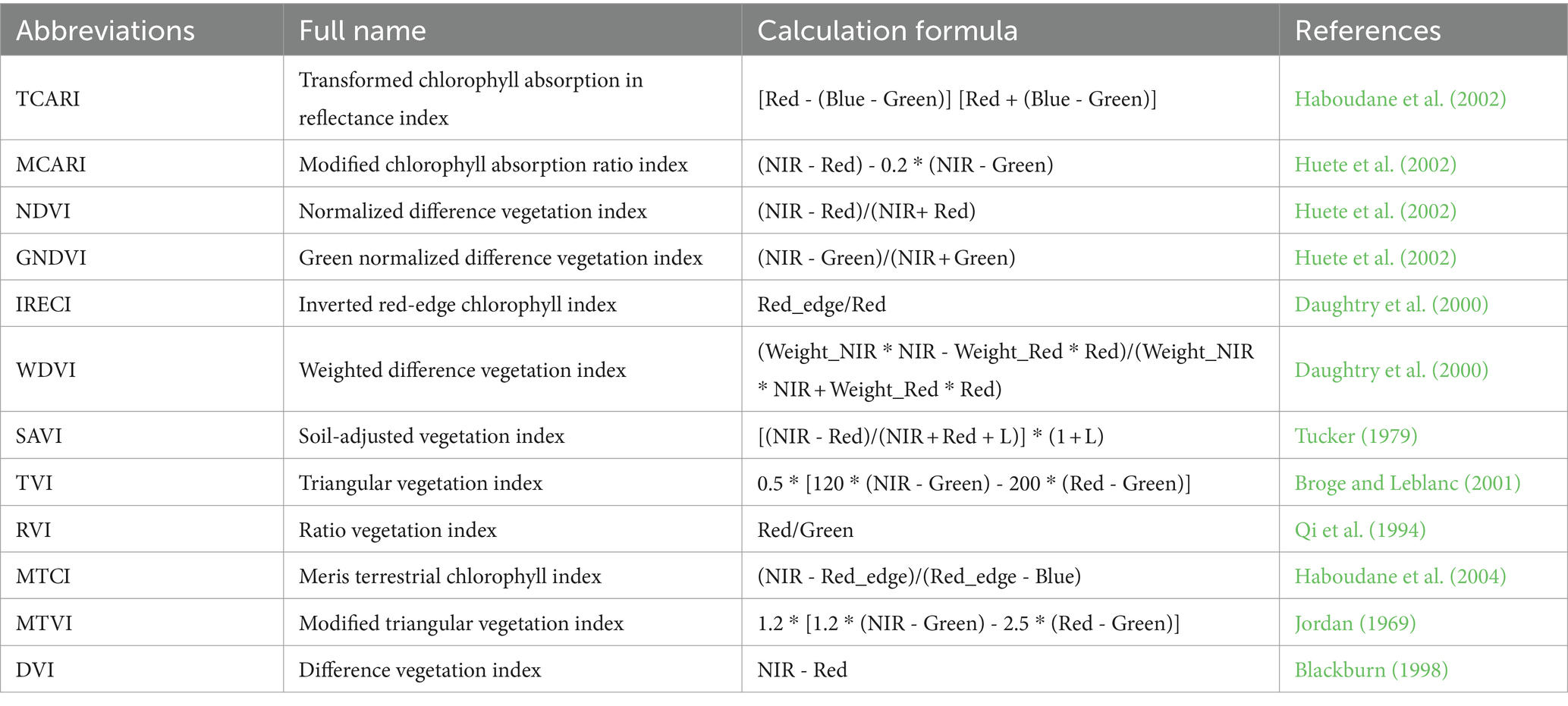
VIs are a type of feature calculated by the linear or nonlinear combination of raw reflectance data (Liang et al., 2015) and are more sensitive to the plants’ growth status than single-band information due to attenuation of environmental background interference in the canopy’s spectrum. In this study, we selected 12 kinds of VIs, which have been widely used previously and have been proven to be highly correlated with the LAI. The description and formulation of the selected indices are shown in Table 2.

Table 2

Table 2. VIs and calculations based on GF-6 WFV data.

2.3.2 Gray level co-occurrence matrices

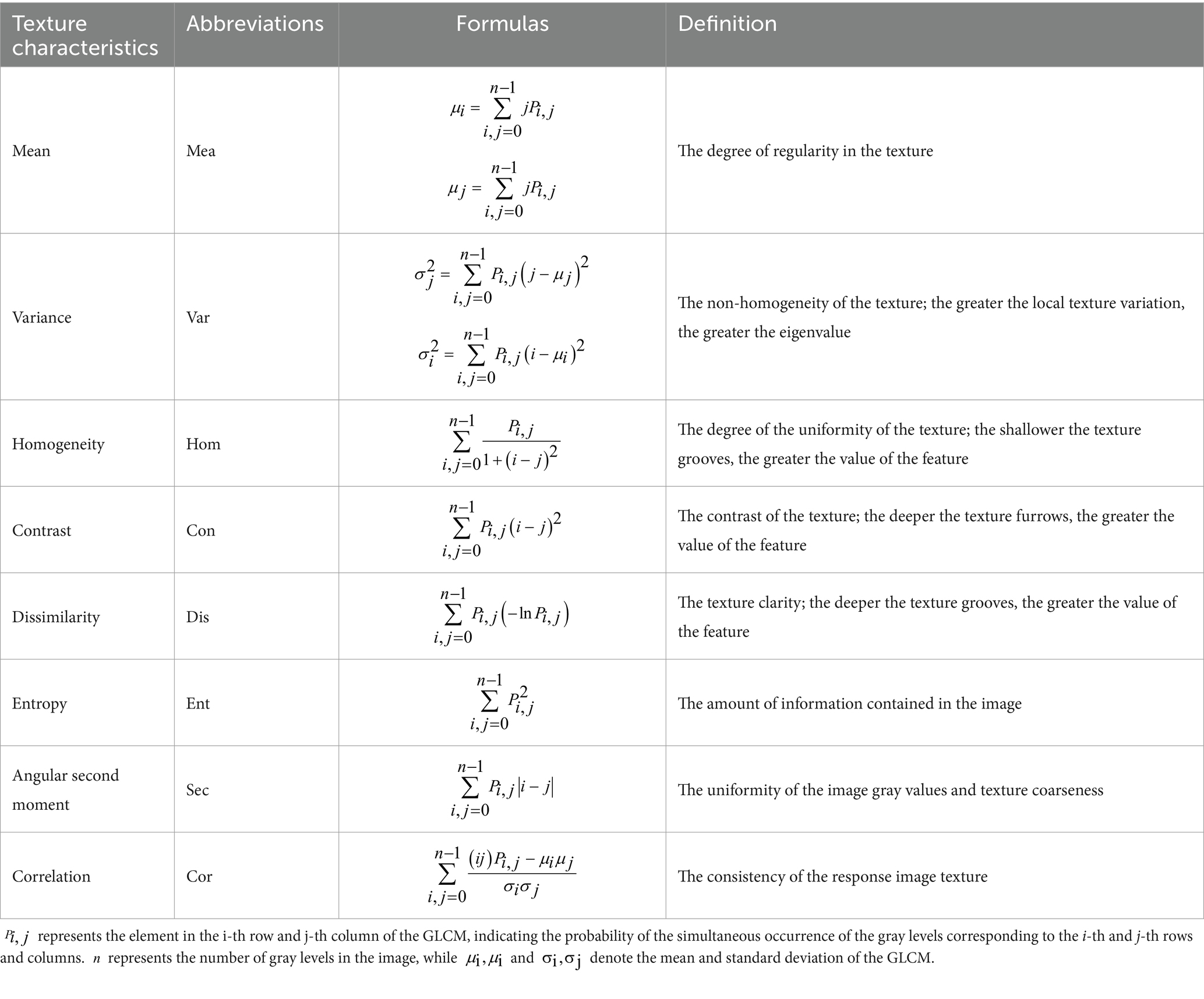
A GLCM contains statistical information about pixel pairs that maintain a certain positional relationship within a local moving window of an image (Haralick et al., 1973), and can be further used to characterize texture information by using various statistical features. It describes the probability distribution of gray level co-occurrence between pixels, providing rich information on image texture and structure, and has become an important measure for LAI estimation from remote sensing imagery. The calculation of GLCM is based on Equation 1:

$P\left(a,b\right)=\left[\begin{array}{l}a=f\left(x,y\right),b=f\left(x+d.\theta ,y+d.\theta \right);\\ a,b\in \left(1,2\cdots n\right);x,y\in \left(R^{H\times W}\right)\end{array}\right]\text{ (1)}$

where a, b denotes the gray level and the maximum gray level is n; thus, the size of the matrix is $\mathrm{n}\times \mathrm{n}$ . The offset direction within a local image window is described by $\theta$ ; the offset distance is d. x, y denotes the pixel coordinates and H, M is the image’s width and height. In all our experiments, N is 64, and the offsets are in four directions, namely 0°, 45°, 90°, 135°, with an offset distance of 1.

In our paper, eight kinds of statistics, namely the mean, variance, homogeneity, contrast, dissimilarity, entropy, angular second-order moments, and autocorrelation, are used to further describe the GLCM, and are detailed in Table 3.

Table 3

Table 3. GLCM texture feature statistics.

It has been reported that parameters such as the size of the moving window and the moving step size will affect the results of the GLCM and further influence the texture feature calculation (Hall-Beyer, 2017). For example, if the size of the moving window is too small, this will lead to erroneous segmentation inside the texture features; on the contrary, erroneous segmentation will occur at the boundary of texture features (Wang et al., 2004). Considering the image characteristics of GF-6 WFV, the size of the moving window and the moving step size are set to 5 and 1, respectively (Marceau et al., 1990). The GLCM texture features are calculated separately for the eight bands of GF-6 WFV; thus, in total, 64 texture features were obtained in our experiments.

2.4 Modeling algorithm

In this study, linear regression and three nonlinear methods were chosen for inversion to compare the accuracy and stability of various models in E. grandis LAI estimation (Andrade et al., 2020). Through this comparison, a more comprehensive exploration of the impacts of VIs and texture characteristics on LAI estimation is possible.

2.4.1 Multiple stepwise regression model

MSR is a rapid and straightforward method for illustrating the relationship between multiple independent variables and the response variable (Liu et al., 2021). This technique involves the step-by-step addition of variables to the model, with each addition predicated on statistical significance to maintain a set of variables that robustly predicts the response variable. The process continues until all variables in the model contribute meaningfully to the prediction, thereby ensuring the selection of an optimal variable set that captures the underlying relationships without including any redundant or insignificant predictors. The resulting regression equation expresses the relationship between the independent and dependent variables, as shown in Equation 2:

$\begin{array}{ll}y=a+x_1{b}_1+x_2{b}_2+\dots x_n{b}_n& (2)\end{array}$

where y is the LAI value (dependent variable), ${\mathrm{x}}_1-{\mathrm{x}}_{\mathrm{n}}$ is the eigenvalue (independent variable), and ${\mathrm{b}}_1-{\mathrm{b}}_{\mathrm{n}}$ is the coefficient of the corresponding independent variable.

2.4.2 Support vector regression model

SVR is a regression method based on support vector machines, specifically designed to predict continuous outputs (Panahi et al., 2020). By seeking the optimal hyperplane and establishing a margin that tolerates a certain amount of error in the training data, SVR utilizes a kernel function to map input data to a high-dimensional space, aiming to identify the maximum margin and enhance tolerance to fluctuations in the training data (Aworka et al., 2022). Commonly used kernel functions include linear, polynomial, and radial basis function (RBF) kernels. While the linear kernel is suitable for linear relationships, polynomial and RBF kernels can handle more complex nonlinear relationships. Additionally, the parameter γ in the RBF kernel significantly influences the kernel width, impacting the model’s complexity. Another crucial parameter is the regularization parameter C, controlling the tolerance for training errors. SVR optimizes these parameters by solving a convex quadratic programming problem, ensuring a balance between fitting the training data and generalizing unseen data. Adjusting these parameters constitutes a critical step when employing SVR (Liu et al., 2021).

2.4.3 Backpropagation neural network model

BPNN is a widely utilized regression algorithm that relies on the concept of backpropagation of errors to minimize the discrepancy between the predicted value and the true value by adjusting the weights in the network (Ding and He, 2003). The BPNN comprises multiple layers, the first of which receives raw data as input, the middle layers, referred to as hidden layers, embed the input into high-dimensional features via interconnected neurons, and the last of which outputs regression values. During the BPNN’s training process, the predicted values of the training dataset are computed through forward propagation, after which, the errors between the predicted and truth values are calculated and backpropagated to update the weights and biases of the network. This iterative process continues until a predetermined number of training sessions is reached or a specified error threshold is reached for the validation dataset.

2.4.4 Random forest model

RF is a data mining technique that combines combinatorial self-learning with modern regression and classification methods, and was introduced by Cutler Adele and Leo Breiman in 2001 (Mohapatra et al., 2020). It is distinguished by its capability to handle large datasets, predict multiple explanatory variables, train data rapidly, and provide variable importance estimates (Jiang et al., 2020). The key problem in RF is to determine the number of RF decision trees (n_tree) and the number of random variables in the split nodes (m_tree). Mtree represents the number of variables selected for each branch of the decision tree, typically set to 1/3 of the number of variables. Moreover, it is crucial not to set n_tree too low to ensure an adequate number of predictions for the sample (Wu et al., 2023a).

2.4.5 Parameter selection and training

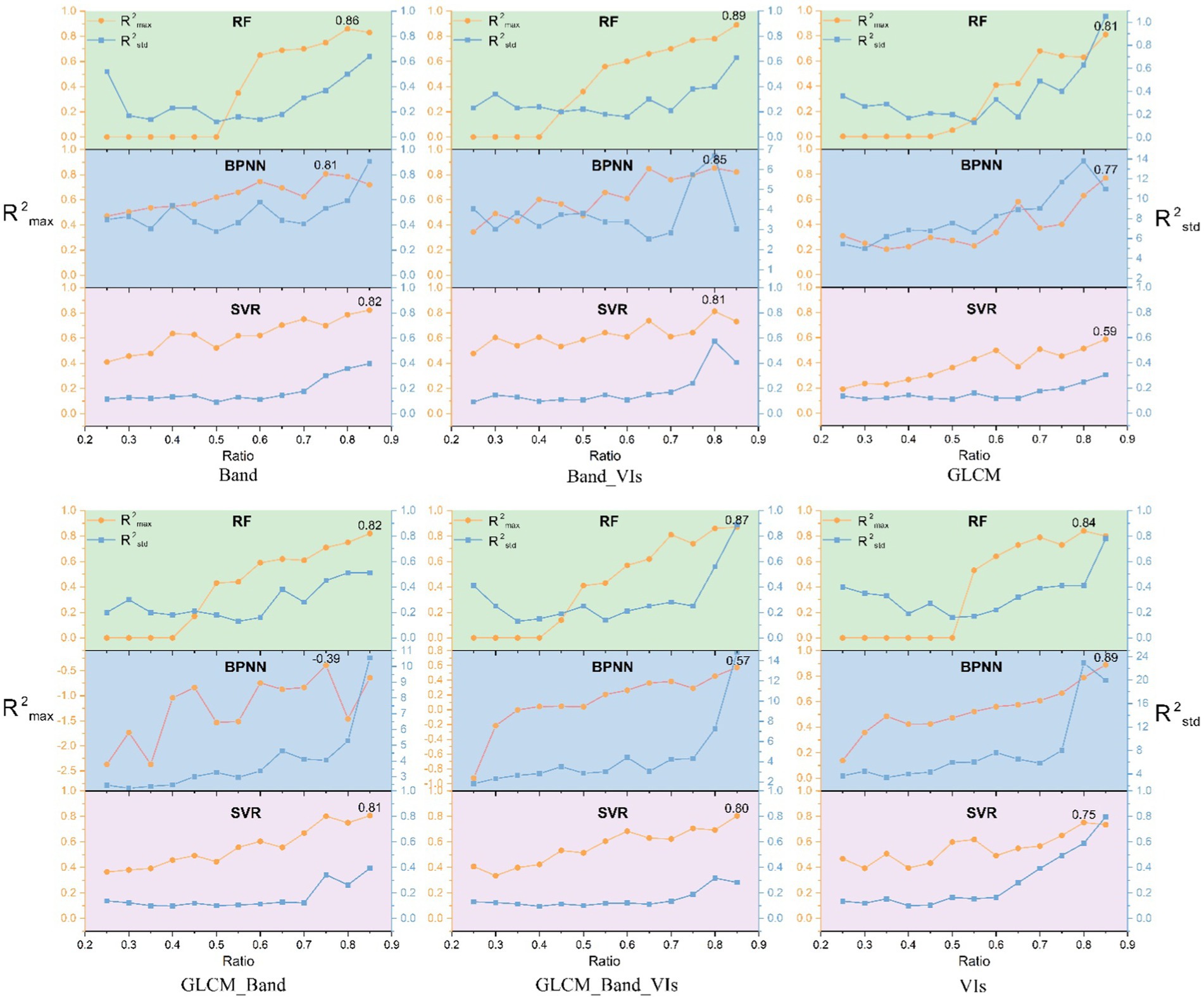
Precise tuning of hyperparameters during ML model construction is a critical step in improving model performance (Yang et al., 2022b). Grid search, a comprehensive and systematic hyperparameter optimization technique, is performed by creating a regular grid of parameters within a defined parameter range. Each coordinate point in this grid represents a unique hyperparameter configuration, and by thoroughly evaluating these configurations, the optimal parameter combinations that maximize model performance can be identified (Sun et al., 2021). For the three nonlinear models (RF, SVR, and BPNN), we employed the grid search method to obtain the optimal combination of hyperparameters for each model. The optimal hyperparameter combination for each machine learning model is selected by grid search technique. Subsequently, to further evaluate the impact of different data splitting ratios on model performance, we designed a series of experiments. The initial splitting rate of the training set was 25%, and then it was incremented in 5% intervals until it reached 85%. For each split rate, the training set was randomly constructed N times and used to train the model. Considering the effectiveness and efficiency, N was set to 100 in all our experiments and the optimal splitting ratio was selected based on the coefficient of determination ( $R_{\text{max}}^2$ ) and standard deviation ( $R_{std}^2$ ) of the models’ performance on the testing set. Finally, these optimal models and splitting ratios were applied to the estimation of E. grandis LAI.

2.4.6 Accuracy evaluation

It is essential to evaluate the fitting status of the models employed in this study to derive the optimal inversion method and to further validate the effectiveness of GF-6 WFV for E. grandis LAI estimation. The fitting status was evaluated using the coefficient of determination (R²) and the root mean square error (RMSE), as recommended in previous studies (Chicco et al., 2021). The calculations of R² and RMSE are based on Equation 3 and 4.

$\begin{array}{ll}{R}^2=1-\frac{{{\displaystyle \sum }}_{i=1}^n{\left(y_i-\widehat{y_j}\right)}^2}{{{\displaystyle \sum }}_{i=1}^n{\left(y_i-\overline{y}\right)}^2}& (3)\end{array}$

$\begin{array}{ll}\mathit{RMSE}=\sqrt{\frac{{{\displaystyle \sum }}_{i=1}^n{\left(\widehat{y_j}-y_i\right)}^2}{n}}& (4)\end{array}$

where ${\mathrm{y}}_{\mathrm{i}}$ denotes the measured E. grandis LAI value, $\widehat{{\mathrm{y}}_{\mathrm{j}}}$ denotes the model-predicted E. grandis LAI value, $\overline{\mathrm{y}}$ denotes the mean value of measured E. grandis LAI, and n denotes the number of samples.

3 Results

3.1 Correlation analysis

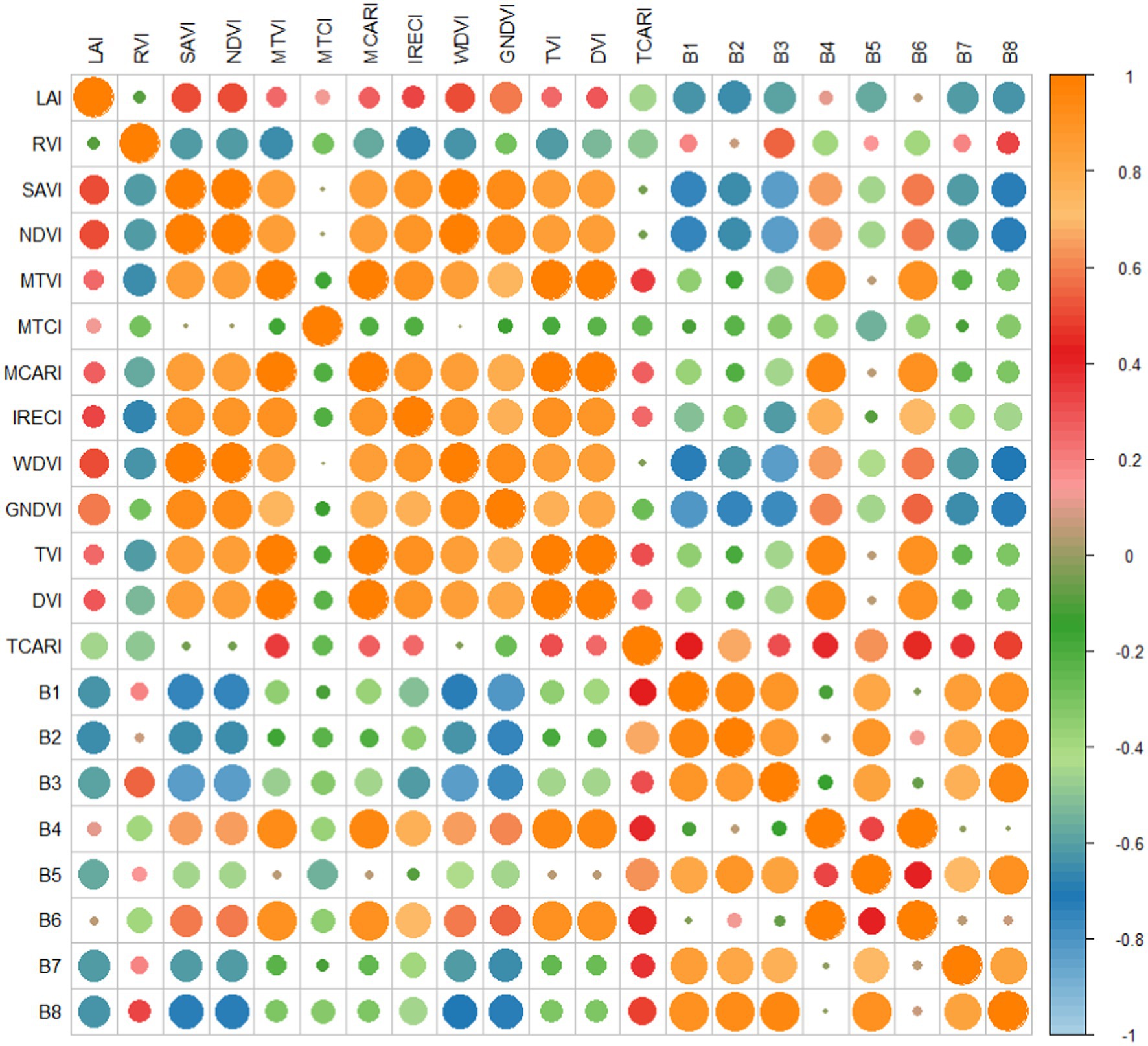
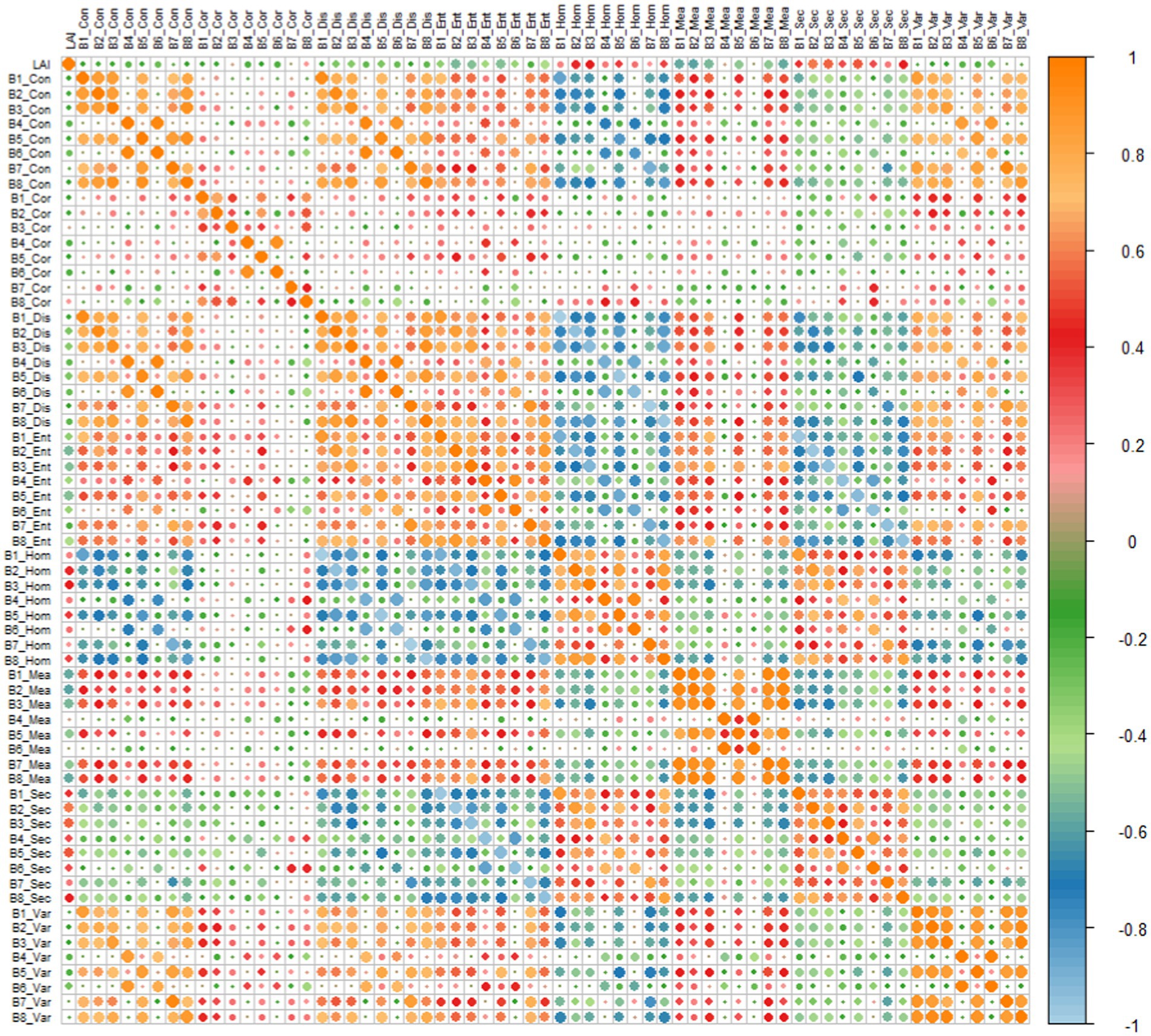
Among 49 sample points in Figure 2B, the maximum value of LAI was 4.47, the minimum value was 0.51, and the mean value was 1.81. Before conducting a reversion analysis, we explored the correlation between the in-put spectral and textural features and the E. grandis LAI and visualized their relationship using the corrplot package in R language (Geitner et al., 2019). This exploration aimed to find features significantly related to LAI estimation, laying the foundation for subsequent model construction.

As illustrated in Figure 3, in total, 7 out of the selected 12 VIs exhibited significant correlations with the E. grandis LAI, of which the GNDVI displayed the highest correlation coefficient of up to 0.58. This validates the excellent performance of VIs in estimating the LAI, especially the key role of the combination of the green band (B2) and the near-infrared band (B4) in the GNDVI in LAI estimation (Janoušek et al., 2023). As for individual spectral features, the B2 band demonstrated the most robust and highest performance among the eight bands, with a correlation coefficient of 0.66. This further validates the outstanding correlation of the green band (B2) in estimating the LAI (Neog, 2023).

Figure 3

Figure 3. Correlation between VIs and E. grandis LAI.

Moreover, an analysis of the GLCM texture feature bands revealed that 30 out of 64 factors displayed significant correlations with E. grandis LAI, as depicted in Figure 4. Among these features, the entropy texture feature (Ent) stood out, with all eight of its bands showing a significant correlation with E. grandis LAI. Notably, the mean texture feature of the green band (B2_Mea) demonstrates the highest significance, with a negative correlation of 0.61 (p < 0.01), which is consistent with the above single-band correlation analysis results. Among the single-band texture features, B2, B3, and B5 showed the most significant correlation with E. grandis LAI, joined by five features (Dis, Ent, Hom, Mea, and Sec) that were significantly correlated with LAI, respectively.

Figure 4

Figure 4. Correlation of texture features with the LAI in E. grandis.

In conclusion, these results indicate significant correlations between the selected VIs and GLCM texture features and E. grandis LAI. This not only affirms the pivotal role of the spectral features of the GF-6 WFV and the texture features of the GLCM in estimating vegetation LAIs, but also provides suggestions for the selection of optimal input factors for subsequent model construction.

Our correlation analysis informed a refined selection of input factors for model construction. We focused on features significantly correlated with the LAI, which included 6 spectral bands, 7 Vegetation Indices (VIs), and 30 GLCM texture features. These factors were combined in seven distinct sets of input parameters, labeled as Band (bands only), VIs (vegetation indices only), G (GLCM texture features only), Band_VIs (combination of bands and vegetation indices), Band_G (combination of bands and GLCM texture features), VIs_G (combination of vegetation indices and GLCM texture features), and Band_VIs_G (combination of bands, VIs, and GLCM texture features). The specific groupings are detailed in Table 4. With this meticulous grouping, we were able to conduct a more detailed estimation and inversion of E. grandis growth, providing more accurate technical support for the monitoring and management of E. grandis plantation forests.

Table 4

Table 4. Parameter groups.

3.2 Linear model—stepwise regression method

The prediction accuracy of the MSR model is closely tied to the correlation coefficients of input factors. In this paper, seven multiple regression models were constructed separately using the parameters in Table 4, and their ability in LAI reversion was evaluated via the R² and RMSE.

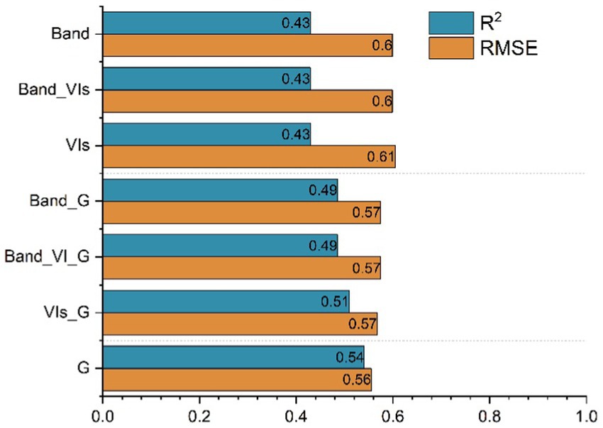
Figure 5 illustrates that the G group, which incorporates GLCM texture features, outperforms other groups in LAI inversion, achieving the highest R² score and the lowest RMSE value at 0.54 and 0.56, respectively. These results surpass the R² scores of both the Band and VIs groups by a notable 11%. The inclusion of texture features significantly bolsters the inversion process, with models utilizing these features witnessing a 7% R² increase and a 3% RMSE decrease on average compared to those without. Additionally, the performance of the Band, VIs, and Band_VIs groups is strikingly similar. This aligns with the understanding that the selected VIs are essentially linear combinations derived from individual bands.

Figure 5

Figure 5. MSR model accuracy evaluation.

3.3 Nonlinear model—machine-learning-based methods

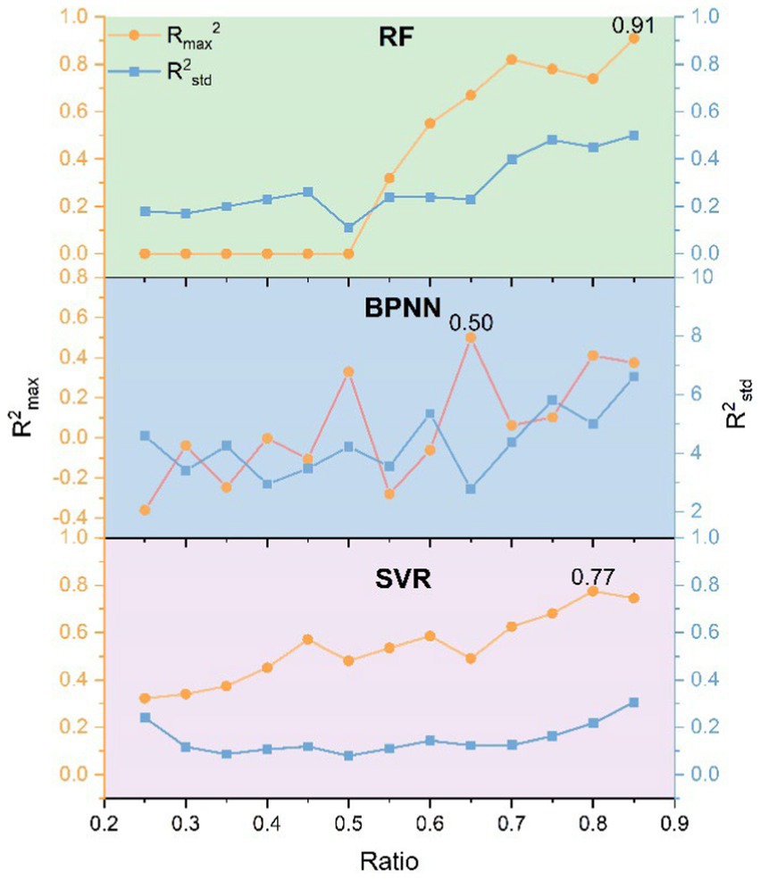
The three selected nonlinear methods (RF, BPNN, and SVR) all use the optimal combination of hyperparameters and then splitting ratios for the dataset of inverted E. grandis LAI. Starting at 25% and increasing in 5% increments to 85%. Data splitting and model training were conducted 100 times randomly for each ratio, and the max and standard deviation of R² of the 100 experiments were used to evaluate the stability and effectiveness of the model at a specific splitting ratio. As shown in Figures 6, 7, the performances of the three models are all influenced by the splitting ratio, which gradually increases as the ratio increases. The $R_{\text{max}}^2$ of the RF model was highest at a splitting ratio of 0.85, with a value of 0.91. That of the BPNN model was highest at a splitting ratio of 0.65, with a value of 0.50, while the $R_{\text{max}}^2$ of the SVR model was highest at a splitting ratio of 0.80, with a value of 0.77. From the aspect of stability, the SVR model is more stable than the other two models, as it has the smallest $R_{std}^2$ at the ratio of the highest $R_{\text{max}}^2$ , more specifically, 0.50, 2.78, and 0.31 for RF, BPNN, and SVR, respectively.

Figure 6

Figure 6. Evaluation of splitting ratio accuracy of nonlinear models based on the VIs_G group.

Figure 7

Figure 7. Evaluation of segmentation ratio accuracy of nonlinear models based on 6 groups.

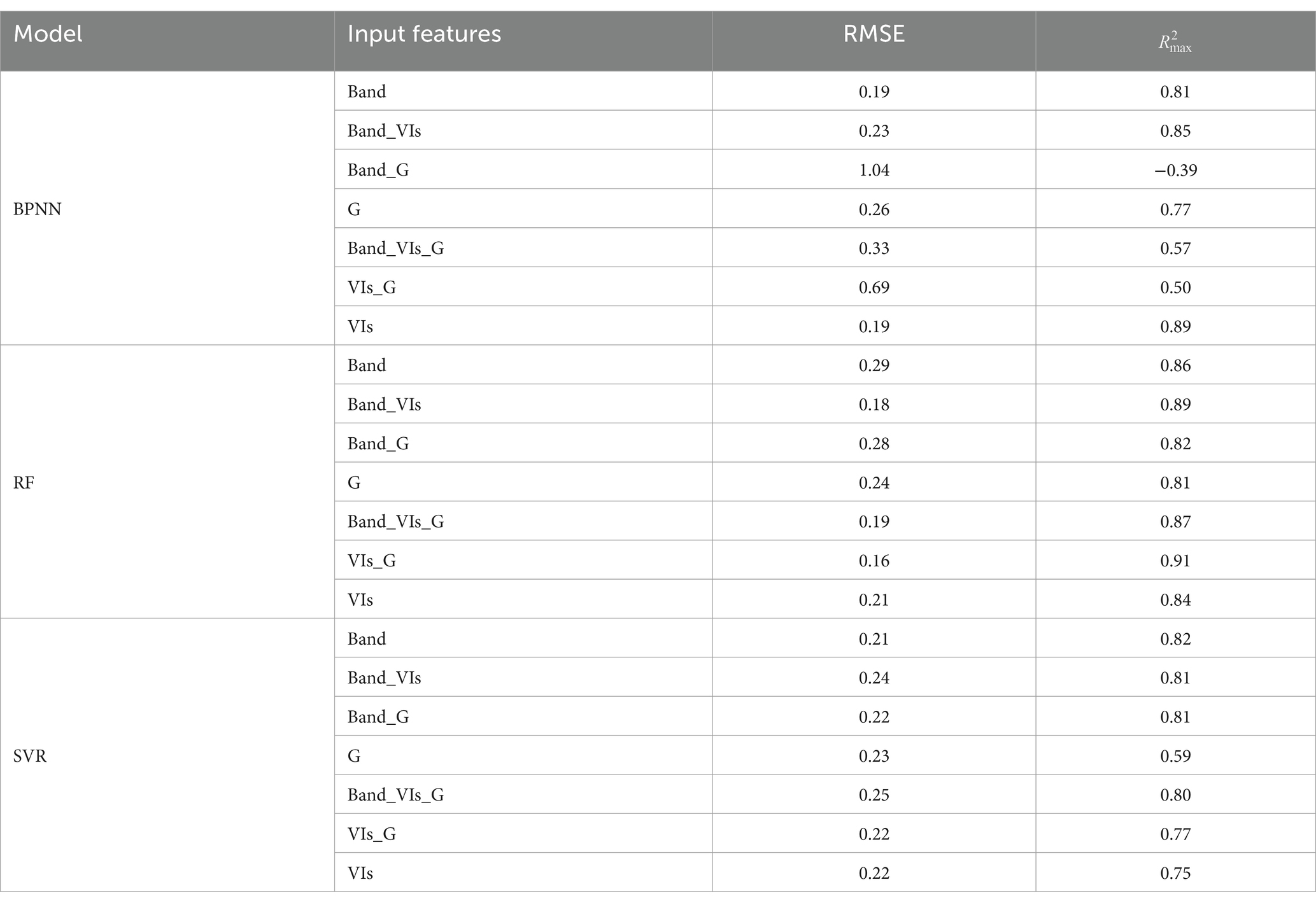
After obtaining the best splitting ratio using the VIs_G group, we directly applied it to the other six input feature groups for LAI inversion, the results of which are shown in Table 5. The VIs_G group excelled in all three models, with a mean $R_{\text{max}}^2$ value of 0.85 and a mean RMSE value of 0.21, which were significantly better than those of the other six groups. Among the three models, the RF’s mean $R_{\text{max}}^2$ for the seven groups of input features (G, Band_G, VIs, Band, VIs_G, and Band_VIs_G groups) was 29 and 10% higher than those of BPNN and SVR, respectively, and its RMSE value was 20 and 1% lower, respectively. The RF model once again demonstrated its superiority in terms of accuracy improvements, with a minimum $R_{\text{max}}^2$ of 0.81, an average value of 0.86 and a maximum value of 0.91, and a mean RMSE of 0.22 and a minimum value of 0.16.

Table 5

Table 5. ML model accuracy evaluation.

Generally, with the 8.5:1.5 splitting ratio, the RF model proved to be more effective for E. grandis LAI inversion, demonstrating a greater overall stability and accuracy, and is more suitable for providing information for monitoring the growing status of E. grandis plantation forests.

4 Discussion

In this study, we utilized GF-6 WFV data to explore the correlation between E. grandis LAI and spectral features as well as GLCM texture features. Through integrating multiple ML methods, we conducted in-depth analysis on these features. Our research initially focused on revealing the correlation between E. grandis LAI and selected remote sensing features, followed by a comparative analysis of different ML modeling techniques. The core objective was to optimize the hyperparameter configuration and data split ratios of the models, thereby significantly improving the accuracy of E. grandis LAI inversion. Through this integrated approach, we aim to develop a more accurate LAI estimation tool to support more effective vegetation monitoring and ecosystem management.

In different input features, combining spectral features with GLCM texture features significantly improves the accuracy of LAI inversion for E. grandis plantations. Spectral features can capture vegetation physiological characteristics, such as chlorophyll content and moisture status, which directly influence vegetation’s light reflection and absorption (Liang et al., 2015). GLCM texture features, on the other hand, reveal vegetation’s spatial distribution patterns, such as tree arrangement and density, which are crucial for understanding and estimating LAI. Especially in E. grandis plantations, the regular planting pattern results in significant differences in texture features at different growth stages. In the sapling stage, the sparse vegetation and similar sizes make texture features particularly prominent. However, in the mature stage, competition among trees leads to uneven distribution and overlapping crowns, resulting in a relative weakening of texture information (Zhou et al., 2013). These texture changes reflect the structural characteristics and growth dynamics of E. grandis trees, closely linked to LAI variations, highlighting the importance of texture features in LAI inversion (Couteron et al., 2005). Therefore, optimizing the use of spectral and texture features can significantly enhance the accuracy of LAI inversion, especially in specific vegetation conditions such as E. grandis plantations, demonstrating substantial potential and application value for this method.

In LAI inversion models, nonlinear models such as RF, BPNN, and SVR demonstrate significant advantages in revealing the complex relationship between input features and LAI. These models are particularly effective in handling the dynamic changes of LAI because LAI is nonlinearly influenced by various biotic and abiotic factors (Reichenau et al., 2016). The superiority of nonlinear models over linear models lies in their ability to capture the complex, non-monotonic relationship between input variables and LAI, including threshold effects, saturation effects, and multi-peak responses (Aworka et al., 2022). Furthermore, nonlinear models can effectively handle interactions among multiple input variables, which is crucial for LAI inversion as there may be complex interaction effects among spectral information, vegetation indices, and texture features (Mohammadpour et al., 2022). The recognition and utilization of these interaction effects significantly enhance the predictive accuracy of nonlinear models. Compared to the MSR model, nonlinear models showed a 26% improvement in R² and a 29% decrease in RMSE. Specifically, RF, BPNN, and SVR models achieved R² improvements of 39, 10, and 29%, respectively, compared to the MSR model, while reducing RMSE values by 36, 16, and 35%, respectively. This further demonstrates the superior performance of nonlinear models in LAI inversion.

In the application of ML models, we extensively explored their potential and limitations in LAI inversion. Despite their significant advantages in pattern recognition and prediction, these models are constrained by the setting of hyperparameters and the strategy for dataset partitioning (Diaz et al., 2017). The high sensitivity of models to these factors may affect their ability to generalize to new data, thereby weakening their accurate prediction of LAI (Joseph and Vakayil, 2022). Unoptimized models are prone to overfitting or underfitting, manifested as performance surplus or deficit on the training set, both of which impair the effective prediction of LAI (Probst et al., 2019). By finely tuning hyperparameters and optimizing the model learning process, we ensure that it can capture the complex relationship between vegetation characteristics and environmental factors more accurately (Weerts et al., 2020). This not only improved the prediction accuracy of the models but also enhanced their adaptability to unknown data. Additionally, through appropriate partitioning of the training and validation sets, we further ensured the robustness and credibility of the models (Roshan et al., 2022). Therefore, the optimization of hyperparameters and the appropriate choice of data partitioning ratio are crucial for enhancing the performance of LAI inversion models. These strategies effectively overcome the inherent limitations of machine learning models and improve their application effectiveness in practical vegetation monitoring and ecological environment assessment.

This study utilized spectral and GLCM texture features from GF-6 WFV data, along with hyperparameter optimization and adjustment of data splitting ratios, to achieve high-precision estimation of LAI in E. grandis plantations. However, we recognize that there is still room for improvement in the model, particularly considering the seasonal variability of LAI in E. grandis plantations, which introduces significant uncertainties. Therefore, there is a need to collect field observation data covering different seasons throughout the year to capture the seasonal changes more accurately in LAI and further optimize the model based on this data. This continuous improvement will enhance the robustness of the model, ensuring reliable support for ongoing environmental monitoring and forestry management. Future work will focus on refining the model to adapt to seasonal variations, thus achieving more accurate LAI inversion under different environmental conditions.

5 Conclusion

In this study, we apply the model’s hyperparameter combination and the debugging method of splitting ratio to investigate the effects of nonlinear modeling and input features on E. grandis plantation forests. In addition, we provide free easy-to-use frameworks for modeling hyperparameter combinations and splitting ratio for debugging methods for fast inversion of E. grandis LAI. First, spectral and GLCM texture features of the GF-6 WFV were used to select features significantly associated with the LAI by correlation analysis. The highest correlation coefficient between GNDVI and spectral features was found to be 0.58. A total of 30 out of 64 GLCM texture features were found to be significantly correlated with LAI, with correlation coefficients up to 0.61. We then conducted comprehensive experiments on different combinations of texture and spectral features using both linear methods and nonlinear models. It was found that using a combination of spectral and GLCM texture features improved accuracy in both linear and nonlinear models, with an 8% improvement and 4% reduction in RMSE for linear and a 6% improvement and 5% reduction in RMSE for nonlinear. In terms of modeling, the nonlinear models significantly outperformed the linear models, with $R_{\text{max}}^2$ averaging 26% higher and RMSE averaging 29% lower for the three nonlinear models. Finally, we searched for the best combination of hyperparameters and conductedexperiments on different dataset splitting ratios, and found that different splitting ratios have a large impact on the accuracy of their models. Among the seven sets of input feature data of the three models, five sets of RF, three sets of BPNN, and four sets of SVR showed high accuracy and stability at a splitting ratio of 8.5:1.5 (ratio of 0.85), with the best $R_{\text{max}}^2$ of 0.91 and $R_{std}^2$ of 0.50 for RF.

This study provides insights in estimating LAI in E. grandis plantation forests by combining the spectral and GLCM texture features of GF-6 WFVs using nonlinear modeling of hyperparameter combinations and splitting ratio debugging methods. Our future research necessitates field measurements in multiple seasons to accurately capture seasonal variations. These additional data will help refine and improve the accuracy of the estimation model and ensure its robustness across seasons. In addition, the optimization of nonlinear methods, the potential effects of different remote sensing data sources, and the effects of plantation species on the accuracy of LAI inversion will be investigated in future work.

Data availability statement

The raw data supporting the conclusions of this article will be made available by the authors, without undue reservation.

Author contributions

XZ: Writing – original draft, Writing – review & editing. BL: Writing – original draft, Writing – review & editing. JH: Writing – original draft, Writing – review & editing. WH: Writing – original draft.

Funding

The author(s) declare that financial support was received for the research, authorship, and/or publication of this article. This research was funded by the National Natural Science Foundation of China (nos. 32101366 and 32060369).

Acknowledgments

We are grateful to the reviewers for their valuable comments and recommendations.

Conflict of interest

The authors declare that the research was conducted in the absence of any commercial or financial relationships that could be construed as a potential conflict of interest.

Publisher’s note

All claims expressed in this article are solely those of the authors and do not necessarily represent those of their affiliated organizations, or those of the publisher, the editors and the reviewers. Any product that may be evaluated in this article, or claim that may be made by its manufacturer, is not guaranteed or endorsed by the publisher.

Footnotes

1. ^https://github.com/BinLiang1/LAI_reversion

References

Andrade, R., Silva, S. H. G., Weindorf, D. C., Chakraborty, S., Faria, W. M., Mesquita, L. F., et al. (2020). Assessing models for prediction of some soil chemical properties from portable X-ray fluorescence (pXRF) spectrometry data in Brazilian Coastal Plains. Geoderma 357:113957. doi: 10.1016/j.geoderma.2019.113957

Crossref Full Text | Google Scholar

Aparicio, N., Villegas, D., Araus, J. L., Casadesús, J., and Royo, C. (2002). Relationship between growth traits and spectral vegetation indices in durum wheat. Crop Sci. 42, 1547–1555. doi: 10.2135/CROPSCI2002.1547

Crossref Full Text | Google Scholar

Aworka, R., Cedric, L. S., Adoni, W. Y. H., Zoueu, J. T., Mutombo, F. K., Kimpolo, C. L. M., et al. (2022). Agricultural decision system based on advanced machine learning models for yield prediction: case of east African countries. Smart Agric. Technol. 2:100048. doi: 10.1016/J.ATECH.2022.100048

Crossref Full Text | Google Scholar

Blackburn, G. A. (1998). Quantifying chlorophylls and Caroteniods at leaf and canopy scales: an evaluation of some hyperspectral approaches. Remote Sens. Environ. 66, 273–285. doi: 10.1016/S0034-4257(98)00059-5

Crossref Full Text | Google Scholar

Broge, N. H., and Leblanc, E. (2001). Comparing prediction power and stability of broadband and hyperspectral vegetation indices for estimation of green leaf area index and canopy chlorophyll density. Remote Sens. Environ. 76, 156–172. doi: 10.1016/S0034-4257(00)00197-8

Crossref Full Text | Google Scholar

Chen, J. M., and Cihlar, J. (1996). Retrieving leaf area index of boreal conifer forests using landsat TM images. Remote Sens. Environ. 55, 153–162. doi: 10.1016/0034-4257(95)00195-6

Crossref Full Text | Google Scholar

Chicco, D., Warrens, M. J., and Jurman, G. (2021). The coefficient of determination R-squared is more informative than SMAPE, MAE, MAPE, MSE and RMSE in regression analysis evaluation. PeerJ Comput. Sci. 7, 1–24. doi: 10.7717/PEERJ-CS.623/SUPP-1

Crossref Full Text | Google Scholar

Couteron, P., Pelissier, R., Nicolini, E. A., and Paget, D. (2005). Predicting tropical forest stand structure parameters from Fourier transform of very high-resolution remotely sensed canopy images. J. Appl. Ecol. 42, 1121–1128. doi: 10.1111/j.1365-2664.2005.01097.x

Crossref Full Text | Google Scholar

Daughtry, C. S. T., Walthall, C. L., Kim, M. S., De Colstoun, E. B., and McMurtrey, J. E. (2000). Estimating corn leaf chlorophyll concentration from leaf and canopy reflectance. Remote Sens. Environ. 74, 229–239. doi: 10.1016/S0034-4257(00)00113-9

Crossref Full Text | Google Scholar

Diaz, G. I., Fokoue-Nkoutche, A., Nannicini, G., and Samulowitz, H. (2017). An effective algorithm for hyperparameter optimization of neural networks. IBM J. Res. Dev. 61, 9:1–9:11. doi: 10.1147/JRD.2017.2709578

Crossref Full Text | Google Scholar

Ding, A. A., and He, X. (2003). Backpropagation of pseudoerrors: neural networks that are adaptive to heterogeneous noise. IEEE Trans. Neural Netw. 14, 253–262. doi: 10.1109/TNN.2003.809428

PubMed Abstract | Crossref Full Text | Google Scholar

Geitner, R., Fritzsch, R., Popp, J., and Bocklitz, T. W. (2019). Corr2d: implementation of two-dimensional correlation analysis in R. J. Stat. Softw. 90, 1–14. doi: 10.18637/JSS.V090.I03

Crossref Full Text | Google Scholar

Haboudane, D., Miller, J. R., Pattey, E., Zarco-Tejada, P. J., and Strachan, I. B. (2004). Hyperspectral vegetation indices and novel algorithms for predicting green LAI of crop canopies: modeling and validation in the context of precision agriculture. Remote Sens. Environ. 90, 337–352. doi: 10.1016/J.RSE.2003.12.013

Crossref Full Text | Google Scholar

Haboudane, D., Miller, J. R., Tremblay, N., Zarco-Tejada, P. J., and Dextraze, L. (2002). Integrated narrow-band vegetation indices for prediction of crop chlorophyll content for application to precision agriculture. Remote Sens. Environ. 81, 416–426. doi: 10.1016/S0034-4257(02)00018-4

Crossref Full Text | Google Scholar

Hall-Beyer, M. (2017). Practical guidelines for choosing GLCM textures to use in landscape classification tasks over a range of moderate spatial scales. Int. J. Remote Sens. 38, 1312–1338. doi: 10.1080/01431161.2016.1278314

Crossref Full Text | Google Scholar

Haralick, R. M., Dinstein, I., and Shanmugam, K. (1973). Textural features for image classification. IEEE Trans. Syst. Man Cybern. SMC-3, 610–621. doi: 10.1109/TSMC.1973.4309314

Crossref Full Text | Google Scholar

Huete, A., Didan, K., Miura, T., Rodriguez, E. P., Gao, X., and Ferreira, L. G. (2002). Overview of the radiometric and biophysical performance of the MODIS vegetation indices. Remote Sens. Environ. 83, 195–213. doi: 10.1016/S0034-4257(02)00096-2

Crossref Full Text | Google Scholar

Iqbal, N., Mumtaz, R., Shafi, U., and Zaidi, S. M. H. (2021). Gray level co-occurrence matrix (GLCM) texture based crop classification using low altitude remote sensing platforms. PeerJ. Comput. Sci. 7, 1–26. doi: 10.7717/PEERJ-CS.536/TABLE-21

Crossref Full Text | Google Scholar

Janoušek, J., Marcoň, P., Dohnal, P., Jambor, V., Synková, H., and Raichl, P. (2023). Predicting the optimum corn harvest time via the quantity of dry matter determined with vegetation indices obtained from multispectral field imaging. Remote Sens. 15:3152. doi: 10.3390/RS15123152

Crossref Full Text | Google Scholar

Jiang, F., Kutia, M., Sarkissian, A. J., Lin, H., Long, J., Sun, H., et al. (2020). Estimating the growing stem volume of coniferous plantations based on random forest using an optimized variable selection method. Sensors 20:7248. doi: 10.3390/S20247248

Crossref Full Text | Google Scholar

Jin, X., Yang, G., Xu, X., Yang, H., Feng, H., Li, Z., et al. (2015). Combined multi-temporal optical and radar parameters for estimating LAI and biomass in winter wheat using HJ and RADARSAR-2 data. Remote Sens. 7, 13251–13272. doi: 10.3390/RS71013251

Crossref Full Text | Google Scholar

Jordan, C. F. (1969). Derivation of leaf-area index from quality of light on the Forest floor. Ecology 50, 663–666. doi: 10.2307/1936256

Crossref Full Text | Google Scholar

Joseph, V. R., and Vakayil, A. (2022). SPlit: an optimal method for data splitting. Technometrics 64, 166–176. doi: 10.1080/00401706.2021.1921037

Crossref Full Text | Google Scholar

Krupnik, T. J., Ahmed, Z. U., Timsina, J., Yasmin, S., Hossain, F., Al Mamun, A., et al. (2015). Untangling crop management and environmental influences on wheat yield variability in Bangladesh: an application of non-parametric approaches. Agric. Syst. 139, 166–179. doi: 10.1016/J.AGSY.2015.05.007

Crossref Full Text | Google Scholar

Liang, L., Di, L., Zhang, L., Deng, M., Qin, Z., Zhao, S., et al. (2015). Estimation of crop LAI using hyperspectral vegetation indices and a hybrid inversion method. Remote Sens. Environ. 165, 123–134. doi: 10.1016/j.rse.2015.04.032

Crossref Full Text | Google Scholar

Liu, Y., Heuvelink, G. B. M., Bai, Z., He, P., Xu, X., Ding, W., et al. (2021). Analysis of spatio-temporal variation of crop yield in China using stepwise multiple linear regression. F. Crop. Res. 264:108098. doi: 10.1016/J.FCR.2021.108098

Crossref Full Text | Google Scholar

Ma, J., Wang, L., and Chen, P. (2022). Comparing different methods for wheat LAI inversion based on hyperspectral data. Agric. 12:1353. doi: 10.3390/agriculture12091353

Crossref Full Text | Google Scholar

Ma, Y., Zhang, Q., Yi, X., Ma, L., Zhang, L., Huang, C., et al. (2021). Estimation of cotton leaf area index (LAI) based on spectral transformation and vegetation index. Remote Sens. 14:136. doi: 10.3390/RS14010136

Crossref Full Text | Google Scholar

Madonsela, S., Cho, M. A., Ramoelo, A., and Mutanga, O. (2017). Remote sensing of species diversity using Landsat 8 spectral variables. ISPRS J. Photogramm. Remote Sens. 133, 116–127. doi: 10.1016/J.ISPRSJPRS.2017.10.008

Crossref Full Text | Google Scholar

Marceau, D. J., Howarth, P. J., Dubois, J. M. M., and Gratton, D. J. (1990). Evaluation of the Grey-level co-occurrence matrix method for land-cover classification using SPOT imagery. IEEE Trans. Geosci. Remote Sens. 28, 513–519. doi: 10.1109/TGRS.1990.572937

Crossref Full Text | Google Scholar

Matese, A., and Di Gennaro, S. F. (2021). Beyond the traditional NDVI index as a key factor to mainstream the use of UAV in precision viticulture. Sci. Rep. 11, 1–13. doi: 10.1038/s41598-021-81652-3

PubMed Abstract | Crossref Full Text | Google Scholar

Mohammadpour, P., Viegas, D. X., and Viegas, C. (2022). Vegetation mapping with random Forest using sentinel 2 and GLCM texture feature—a case study for Lousã region, Portugal. Remote Sens. 14:585. doi: 10.3390/RS14184585

Crossref Full Text | Google Scholar

Mohapatra, N., Shreya, K., and Chinmay, A. (2020). Optimization of the random forest algorithm. Lect. Notes Data Eng. Commun. Technol. 37, 201–208. doi: 10.1007/978-981-15-0978-0_19

Crossref Full Text | Google Scholar

Myburg, A. A., Grattapaglia, D., Tuskan, G. A., Hellsten, U., Hayes, R. D., Grimwood, J., et al. (2014). The genome of Eucalyptus grandis. Nature 510, 356–362. doi: 10.1038/nature13308

Crossref Full Text | Google Scholar

Neog, R. (2023). Fury of nature: evaluating the impact of hailstorm on vegetation using sentinel 2 data at Moran, India. Acta Geophys. 71, 3025–3039. doi: 10.1007/s11600-023-01138-w

Crossref Full Text | Google Scholar

Nguyen, Q. H., Ly, H., Ho, L. S., Al-ansari, N., Van Le, H., Tran, V. Q., et al. (2021). Influence of data splitting on performance of machine learning models in prediction of shear strength of soil. Mathematic. Prob. Eng. 2021, 1–15. doi: 10.1155/2021/4832864

Crossref Full Text | Google Scholar

Ouyang, L., Zhao, P., Zhou, G., Zhu, L., Huang, Y., Zhao, X., et al. (2018). Stand-scale transpiration of a Eucalyptus urophylla × Eucalyptus grandis plantation and its potential hydrological implication. Ecohydrology 11:1938. doi: 10.1002/eco.1938

Crossref Full Text | Google Scholar

Padalia, H., Sinha, S. K., Bhave, V., Trivedi, N. K., and Senthil Kumar, A. (2020). Estimating canopy LAI and chlorophyll of tropical forest plantation (North India) using Sentinel-2 data. Adv. Sp. Res. 65, 458–469. doi: 10.1016/J.ASR.2019.09.023

Crossref Full Text | Google Scholar

Panahi, M., Sadhasivam, N., Pourghasemi, H. R., Rezaie, F., and Lee, S. (2020). Spatial prediction of groundwater potential mapping based on convolutional neural network (CNN) and support vector regression (SVR). J. Hydrol. 588:125033. doi: 10.1016/J.JHYDROL.2020.125033

Crossref Full Text | Google Scholar

Probst, P., Boulesteix, A. L., and Bischl, B. (2019). Tunability: Importance of hyperparameters of machine learning algorithms. J. Mach. Learn. Res. 20, 1–32. doi: 10.5555/3322706.3361994

Crossref Full Text | Google Scholar

Qi, J., Chehbouni, A., Huete, A. R., Kerr, Y. H., and Sorooshian, S. (1994). A modified soil adjusted vegetation index. Remote Sens. Environ. 48, 119–126. doi: 10.1016/0034-4257(94)90134-1

Crossref Full Text | Google Scholar

Reichenau, T. G., Korres, W., Montzka, C., Fiener, P., Wilken, F., Stadler, A., et al. (2016). Spatial heterogeneity of leaf area index (LAI) and its temporal course on arable land: combining field measurements, remote sensing and simulation in a comprehensive data analysis approach (CDAA). PLoS One 11:e0158451. doi: 10.1371/journal.pone.0158451

PubMed Abstract | Crossref Full Text | Google Scholar

Roshan, V., Stewart, J. H. M., Joseph, R., and Stewart, H. M. (2022). Optimal ratio for data splitting. Stat. Anal. Data Min. ASA Data Sci. J. 15, 531–538. doi: 10.1002/SAM.11583

Crossref Full Text | Google Scholar

Sun, Y., Ding, S., Zhang, Z., and Jia, W. (2021). An improved grid search algorithm to optimize SVR for prediction. Soft. Comput. 25, 5633–5644. doi: 10.1007/s00500-020-05560-w

Crossref Full Text | Google Scholar

Tesfamichael, S. G., Aardt, J.Van, Roberts, W., and Ahmed, F. (2018). Retrieval of narrow-range LAI of at multiple lidar point densities: Application on Eucalyptus grandis plantation. Int. J. Appl. Earth Obs. Geoinf. 70, 93–104. doi: 10.1016/j.jag.2018.04.014

Crossref Full Text | Google Scholar

Tucker, C. J. (1979). Red and photographic infrared linear combinations for monitoring vegetation. Remote Sens. Environ. 8, 127–150. doi: 10.1016/0034-4257(79)90013-0

Crossref Full Text | Google Scholar

Tuominen, S., and Pekkarinen, A. (2005). Performance of different spectral and textural aerial photograph features in multi-source forest inventory. Remote Sens. Environ. 94, 256–268. doi: 10.1016/j.rse.2004.10.001

Crossref Full Text | Google Scholar

Wang, X., Cai, G., Lu, X., Yang, Z., Zhang, X., and Zhang, Q. (2022). Inversion of wheat leaf area index by multivariate red-edge spectral vegetation index. Sustain. For. 14:15875. doi: 10.3390/su142315875

Crossref Full Text | Google Scholar

Wang, L., Sousa, W. P., Gong, P., and Biging, G. S. (2004). Comparison of IKONOS and QuickBird images for mapping mangrove species on the Caribbean coast of Panama. Remote Sens. Environ. 91, 432–440. doi: 10.1016/j.rse.2004.04.005

Crossref Full Text | Google Scholar

Weerts, H. J. P., Mueller, A. C., and Vanschoren, J. (2020). Importance of Tuning Hyperparameters of Machine Learning Algorithms. arXiv.org. doi: 10.48550/arXiv.2007.07588

Crossref Full Text | Google Scholar

Wu, N., Crusiol, L. G. T., Liu, G., Wuyun, D., and Han, G. (2023a). Comparing the performance of machine learning algorithms for estimating aboveground biomass in typical steppe of northern China using sentinel imageries. Ecol. Indic. 154:110723. doi: 10.1016/j.ecolind.2023.110723

Crossref Full Text | Google Scholar

Wu, X., Zhang, X., Heki, K., Wei, H., Yang, X., Pan, Y., et al. (2023b, 2023). GNSS-IR soil moisture inversion derived from multi-GNSS and multi-frequency data accounting for vegetation effects. Remote Sens. 15:5381. doi: 10.3390/RS15225381

Crossref Full Text | Google Scholar

Xia, T., He, Z., Cai, Z., Wang, C., Wang, W., Wang, J., et al. (2022). Exploring the potential of Chinese GF-6 images for crop mapping in regions with complex agricultural landscapes. Int. J. Appl. Earth Obs. Geoinf. 107:102702. doi: 10.1016/j.jag.2022.102702

Crossref Full Text | Google Scholar

Yang, H., Guo, H., Dai, W., Nie, B., Qiao, B., and Zhu, L. (2022a). Bathymetric mapping and estimation of water storage in a shallow lake using a remote sensing inversion method based on machine learning. Int. J. Digit. Earth 15, 789–812. doi: 10.1080/17538947.2022.2069873

Crossref Full Text | Google Scholar

Yang, Z., Lv, H., Xu, Z., and Wang, X. (2022b). Source discrimination of mine water based on the random forest method. Sci. Rep. 12, 1–12. doi: 10.1038/s41598-022-24037-4

PubMed Abstract | Crossref Full Text | Google Scholar

Yang, W. N., Qin, Z. T., Yang, X., Jian, J., Li, Y. X., and Pan, P. F. (2015). Novel quantitative measurement of eco-water layer based on quantitative remote sensing. J. Comput. Theor. Nanosci. 12, 2837–2841. doi: 10.1166/JCTN.2015.4186

Crossref Full Text | Google Scholar

Yang, L., and Shami, A. (2020). On hyperparameter optimization of machine learning algorithms: theory and practice. Neurocomputing 415, 295–316. doi: 10.1016/j.neucom.2020.07.061

Crossref Full Text | Google Scholar

Yao, Y., Huang, J., He, W., Zhu, J., and Li, Y. (2023). Changes in water-use efficiency of Eucalyptus plantations and its driving factors in a Small County in South China. Water 15, 1–13. doi: 10.3390/w15152754

Crossref Full Text | Google Scholar

Zhang, J., Qiu, X., Wu, Y., Zhu, Y., Cao, Q., Liu, X., et al. (2021). Combining texture, color, and vegetation indices from fixed-wing UAS imagery to estimate wheat growth parameters using multivariate regression methods. Comput. Electron. Agric. 185:106138. doi: 10.1016/J.COMPAG.2021.106138

Crossref Full Text | Google Scholar

Zhou, J., Proisy, C., Descombes, X., le Maire, G., Nouvellon, Y., Stape, J. L., et al. (2013). Mapping local density of young Eucalyptus plantations by individual tree detection in high spatial resolution satellite images. For. Ecol. Manag. 301, 129–141. doi: 10.1016/j.foreco.2012.10.007

Crossref Full Text | Google Scholar