A live fuel moisture climatology in California

In this study, observations of live fuel moisture content (LFMC) for predominantly sampled fuels in six distinct regions of California were examined from 2000 to 2021. To gather the necessary data, an open-access database called the Fuel Moisture Repository (FMR), was developed. By harnessing the extensive data aggregation and query capabilities of the FMR, which draws upon the National Fuel Moisture Database, valuable insights into the live fuel moisture seasonality were obtained. Specifically, our analysis revealed a distinct downtrend in LFMC across all regions, with the exception of the two Northernmost regions. The uptrends of LFMC seen in those regions are insignificant to the general downtrend seen across all of the regions. Although the regions do not share the same trends over the temporal span of the study, from 2017 to 2021, all the regions experienced a downtrend two times more severe than the general 22-year downtrend. Further analysis of the fuel types in each of the six regions, revealed significant variability in LFMC across different fuel types and regions. To understand potential drivers of this variability, the relationship between LFMC and drought conditions was investigated. This analysis found that LFMC fluctuations were closely linked to water deficits. However, the drought conditions varied across the examined regions, contributing to extreme LFMC variability. Notably, during prolonged drought periods of 2 or more years, fuels adapted to their environment by stabilizing or even increasing their maximum and minimum moisture values, contrary to the expected continual decrease. These LFMC trends have been found to correlate to wildfire activity and the specific LFMC threshold of 79% has been proposed as trigger of an increased likelihood of large fires. By analyzing the LFMC and fire activity data in each region, we found that more optimal local thresholds can be defined, highlighting the spatial variability of the fire response to the LFMC. This work expands on existing literature regarding the connections between drought and LFMC, as well as fire activity and LFMC. The study presents a 22-year dataset of LFMC spanning the entirety of California and analyses the LFMC trends in California that haven’t been rigorously studied before.

1. Introduction

Wildfires play an integral role in ecosystems all around the globe by increasing biodiversity and regulating water availability (Rollins et al., 2004; Chuvieco et al., 2009; Deák et al., 2014; Pausas and Keeley, 2019). Unfortunately, as urban development spreads into wildland areas, these regions become prone to wildfires which in turn, place heavy burdens on local economies, air quality, and citizen health (Crutzen and Andreae, 1990; Lelieveld et al., 2015, Rao et al., 2020). These problems have been amplified as a results of recent increase in fire activity, motivating studies assessing the potential for wildfires in connection to weather and fuel conditions. Although several factors such as fuel type, wind speed, and slope contribute to wildfire danger, the fuel moisture content (FMC) has been recognized as one of the most critical ones (Chuvieco et al., 2009). FMC is defined as the amount of water in a fuel relative to its dry weight (Matthews, 2014). As there is a certain amount of energy required to evaporate water, FMC in part regulates the effective heat release of burning fuel. This then influences various fire characteristics such as the energy needed for ignition, flammability, fuel consumption, and rate of spread (RoS) (Rothermel, 1972; Dimitrakopoulos and Papaioannou, 2001; Chatelon et al., 2022). Therefore, FMC is critical for fire management in the context of fire spread prediction as well as fire danger and risk assessment.

FMC is divided into two categories, dead fuel moisture content (DFMC), and live fuel moisture content (LFMC). Dead fuels are mainly affected by meteorological conditions, with their drying and moistening rates depending on the fuel size class corresponding to the time lag typically defined as 1 h, 10 h, 100 h, and 1,000 h for fuels in sizes ranging from less than 0.25 inch to more than 3 inches in diameter. While the DFMC can be calculated using meteorological parameters (van Wagner, 1987; Nelson, 2000; Mandel et al., 2012, Vejmelka et al., 2016), due to the more complex dynamics of live fuels, estimating their moisture content based on meteorological conditions alone is problematic. That is because live fuels are also affected by climate trends, plant physiology, soil moisture, and evapotranspiration (Pollet and Brown, 2007; Qi et al., 2012; Matthews, 2014). An example of this complexity can be seen when plants close their stomata to reduce moisture loss via the evapotranspiration process, they reduce their dependence on environmental conditions (van der Molen et al., 2011). The LFMC can vary, both spatially and temporally (Danson and Bowyer, 2004) differently than DFMC and be less dependent on short-term weather conditions (Viegas et al., 2001). The LFMC can be assessed by collecting fuel samples, computing their water content by subtracting the oven dry weight from the wet weight, and normalizing the computed water content by the dry mass. This procedure requires destructive sampling and is very labor intensive. That is why at most fuel moisture content of live fuels is sampled only biweekly or monthly. Also, since the drying process of the fuels takes 24 h, unlike dead fuels which may be sampled automatically by dead fuel moisture sensors reporting near-real time data to weather stations, live fuel moisture data are available at much lower frequency and with significant delay.

Since the direct non-destructive sampling of live fuel moisture is not viable, the only alternative method of LFMC assessment is remote sensing. Using satellite data to estimate LFMC provides high spatial coverage and relatively high temporal resolution compared to the regular fuel sampling performed at 14-day to month time intervals (Yebra et al., 2013). An example of such a product is an operational remote sensing fuel moisture leveraging machine learning model created by McCandless et al. (2020). Although this model provides a daily, 1-kilometer gridded FMC dataset for the Continental United States (CONUS), it suffers from up to 33% error in some areas, and a short time record, that precludes long-term analyses. The development and validation of models such as this one is also contingent upon the sampling of live fuels. Due to the models’ limitations in the context of accuracy, and the short data records constrained by the availability of satellite observations, fuel sampling is still the best option for obtaining local data suitable for analysis of the long-term (climatological) trends.

There has also been attempts to predict and model LFMC by correlating external factors such as drought to LFMC. Water availability plays a key role in the vegetation growth cycle. With both, limited soil moisture and little precipitation impacting plant water intake, drought conditions play a crucial role in LFMC (Dennison et al., 2003; Nolan et al., 2018, 2020). Both Pellizzaro et al. (2007) and Ruffault et al. (2018) looked into this potential relationship. They found that meteorological drought indices such as the Duff Moisture Code and Drought Code of the Canadian Forest Fire Weather Index System as well as the Keetch-Byram Drought Index can be correlated to LFMC trends. The correlation between drought and LFMC has significant implications for predicting and modeling LFMC, which, in turn, plays a crucial role in wildfire growth dynamics.

One field study conducted by Dennison and Moritz (2009) investigated such wildfire growth dynamics wherein they compared LFMC to the burned area in the Santa Monica Mountains and found that large wildfires (which they defined as 1,000 hectares or more) were more likely to occur when LFMC of Mediterranean, shrub-dominated fuels dropped to or below a threshold of 79%. The approximate time that the threshold occurred was correlated to antecedent rainfall during the early months of a given year. The critical LFMC threshold has been applied to other studies around the globe with varying results. A study conducted in Southeastern Australia by Nolan et al. (2016) found that local LFMC thresholds were greater (between 79–111%) than the 79% value reported by Dennison and Moritz (2009). While previous studies have suggested that LFMC plays a significant role in regulating the occurrence of large wildfires, the spatial variability of these thresholds and the seasonal patterns and long-term trends in LFMC remain unclear.

Although Bowers (2018) examined LFMC trends in relation to the fire activity at few sites, no study has looked at the seasonality of LFMC, in connection to fire activity and drought across all of California. This is in-part due to the inadequate amount of LFMC available to conduct such a study and technical difficulties with the data acquisition and processing. Recently, about 20 years of LFMC data has become available through the NFMD and a new data repository (described in this study) has been created to streamline LFMC analyses.

In this study, we adopt the definition of climatology as a term which refers to “the same atmospheric processes as meteorology, but it seeks to identify the slower-acting influences and longer-term changes,” and which “involves a statistical analysis of the various weather elements, such as temperature, moisture, atmospheric pressure, and wind speed” (The Editors of Encyclopaedia Britannica, 2015). Here, we specifically extended this definition to live fuel moisture, and use the term “live fuel moisture climatology,” to describe the long-term changes in the water content of live fuels.

Using this framework, our paper focused on the analysis of live fuel moisture in six bioregions of California from 2000 to 2021. We examined the seasonality and long-term trends in live fuel moisture, considering both the maximum and minimum values, as well as general yearly trends. The analysis was performed for the whole available data records as well as just the last 5 years (2017–2021) to explore recent upticks in fire trends. Additionally, in order to understand the underlying factors driving the LFMC trends, we evaluated the concurrent climatological drought conditions alongside LFMC. The study concludes by examining the correlation between large wildfire potential and LFMC, while also analyzing the spatial variability in the critical LFMC levels that trigger the occurrence of large fires.

2. Data and methods

2.1. Fuel moisture repository

The NFMD is a website application that has a query system that allows users to access live- and dead-fuel moisture information used in wildland fire management (Delgado, 2009). The application uses a database that is updated by fuel specialists who observe, sample, collect, and input the fuel moisture data into the NFMD. To optimize data acquisition, and querying needed for the long-term live fuel moisture analysis, the Fuel Moisture Repository (FMR) has been created. The FMR creates a repository on a local machine and optimizes the storage of the data acquired from the NFMD. The local database is controlled by the dedicated script FMR.py, which is available on a public GitHub repository at https://github.com/wirc-sjsu/FMR. The script subsets the desired data by regions (e.g., States, GACC, or every region), acquires data from the NFMD, organizes the data by year, and creates a local repository. This data is then readily available to the user whenever they may need it. From here, the user can query the data by timeframe, stations ID, fuel species [fuel types (Chamise, Manzanita, Sagebrush, etc.) and fuel variations (new growth, old growth, whitethorn, etc.)], and geolocation (bounding box) using the Example_FMR_Code.py script. Based on the requested criteria, the script packages all the requested data into a CSV file with the name of the file being the timestamp indicating when it was created. The workflow outlined above allows for easy selection and organization of the LFMC data and was used in this study.

2.2. Regions

California is the third largest state in the United States by land mass and has a Mediterranean climate. Some regions are heavily forested while other regions experience significant aridity leading to extended grasslands and desert areas. These conditions provide diverse ecosystems across the state. The California State Water Resources Control Board divided California into 10 different bioregions based on topography and local ecosystems. Modifying these divisions, we refined spatial classification by creating a total of 9 different regions: Klamath (KLA), Modoc (MOD), Sacramento (SAC), Bay Area (BA), Sierra Nevada (SN), Central Coast (CC), San Joaquin Valley (SJV), South Coast (SC), and the Mojave Desert (MD), as seen in Figure 1. The collected data for this study has been categorized according to each respective region. During the initial analysis of LFMC in each region, a few areas (Mojave Desert, Sacramento, and San Joaquin Valley) were identified with minimal or no observations and were subsequently excluded. Thus, this study focuses solely on the six regions (KLA, MOD, BA, SN, CC, and SC) that possess a substantial amount of LFMC data.

FIGURE 1

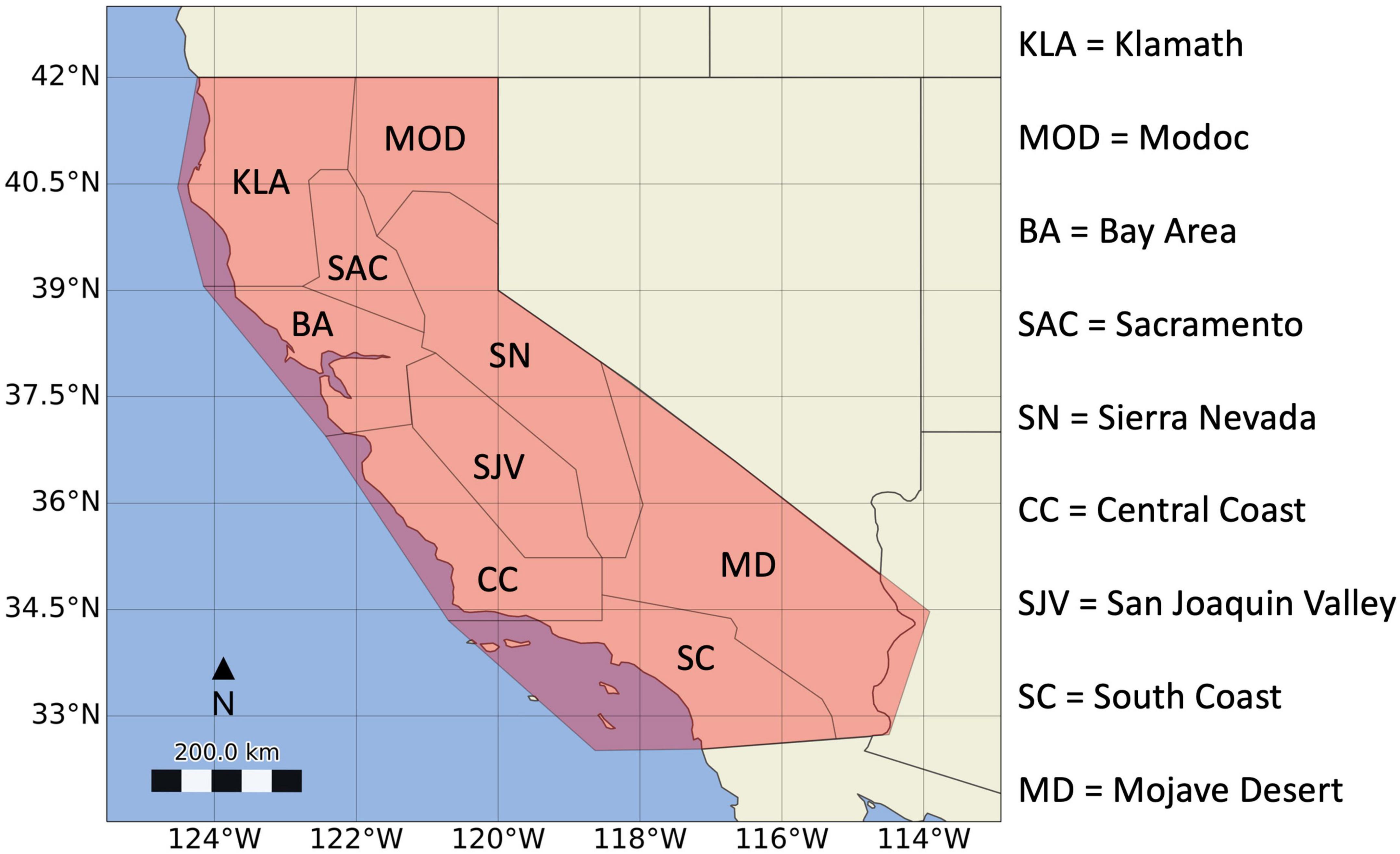
Figure 1. The boundaries of regions utilized in this study. The explanation of the region codes is presented in the legend next to the figure.

2.3. LFMC climatology

The FMR was used to gather and subset the LFMC data from sites within the regions’ boundaries described above (Section “2.2. Regions”). Most of the regions had a diverse range of live fuels and the start times of the data records for those fuels varied from region to region (Table 1). Using one of the FMR’s built-in plotting functions, a bar plot displaying regional variability in the types of fuels as well as the number of observations was used to find the most abundant and representative fuel type in each region. To examine the spatial variability of the live fuel moisture, we separately analyzed the climatology across each of the geographical regions. The climatology of the fuels was broken into two sections, seasonality, and long-term trends. For the seasonality figures (Figures 2, 3), all the fuel data were grouped by month and then averaged across the analyzed years to account for all the observations each month. The long-term trend figures depicted in Figures 4–7 showcase the annual maxima, annual minima, and general trends (annually averaged values). Figures 4, 5 provide an overview of the long-term trends spanning the entire research period from 2000 to 2021, while Figures 6, 7 focus specifically on the trends observed in the last 5 years (2017-2021). The corresponding numerical representation of these trends can be found in Supplementary Tables 1–3 in the Appendix. To find the annual maximum trend, we identified the maximum monthly averaged fuel moisture values for each year and applied a simple linear regression model to those values. A similar process was applied to the annual minimum and general fuel moisture trends. To corroborate the results seen from the linear regression model, we also ran the Mann-Kendall Test (Hamed and Ramachandra Rao, 1998). After examining the LFMC data alone, we analyzed the data against two other datasets; first, we looked at how drought affects the annual maximum and minimum values of LFMC (Section “2.4. Drought impact on LFMC”), and second, we compared the number of large wildfires to LFMC values (Section “2.5. Burned area”).

TABLE 1

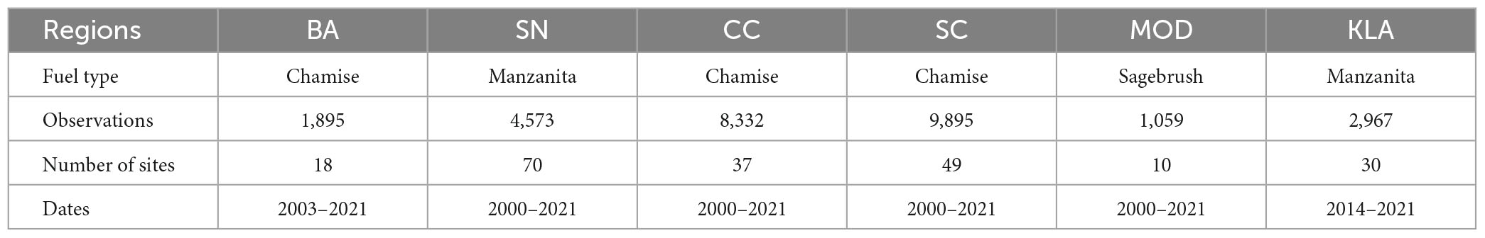
Table 1. The fuel type most extensively sampled in each region, the number of observations of that given fuel, number of sites within each region, and when the collection of the data started relative to our 2000–2021 study.

FIGURE 2

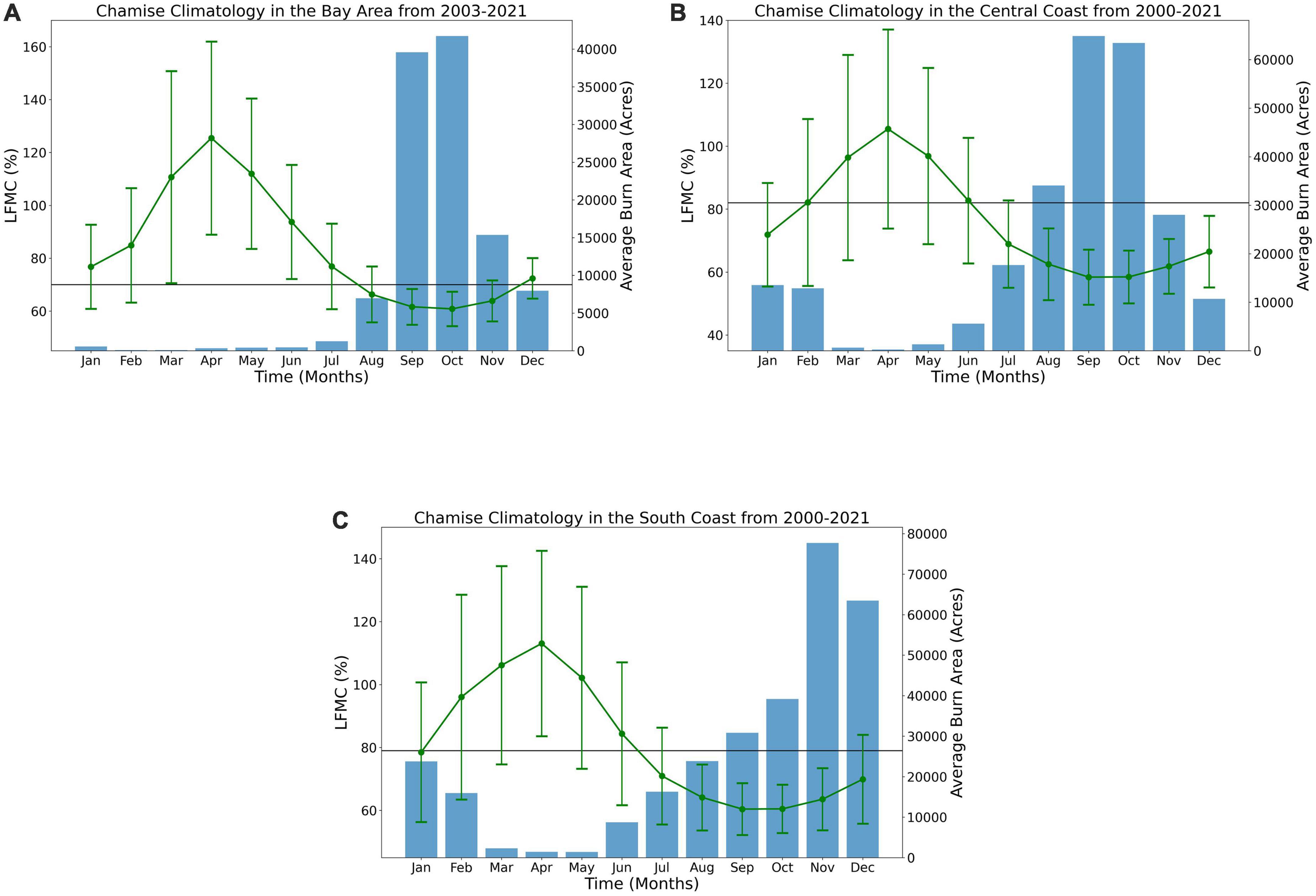
Figure 2. Annually averaged LFMC (horizontal green line), standard deviation of the data (vertical green lines with caps), annually averaged burned area for each month (blue bars), the LFMC threshold (horizontal black line), for the (A) Bay Area, (B) Central Coast, and (C) South Coast regions. The analyzed time ranges are indicated in the headers of each plot.

FIGURE 3

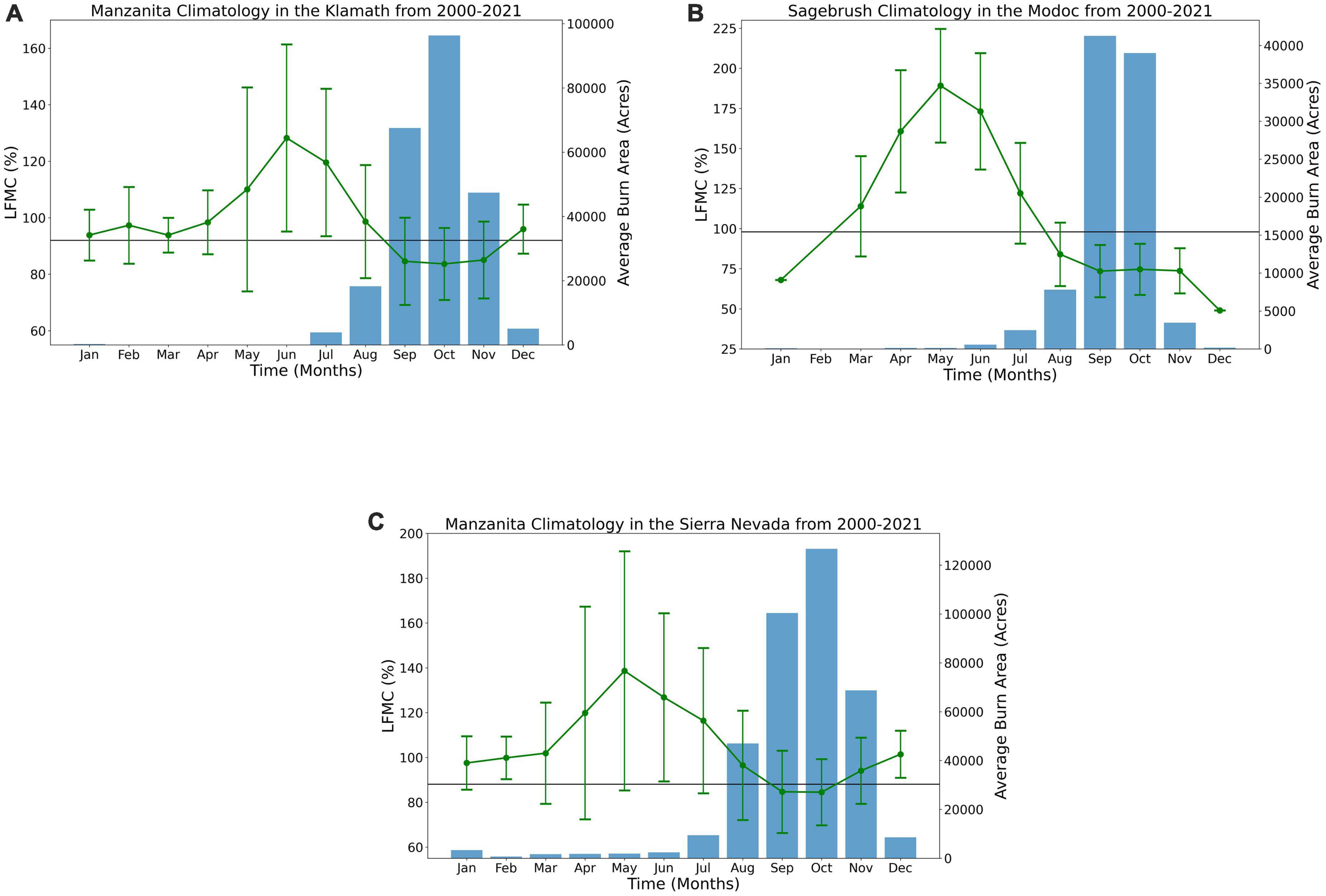
Figure 3. Annually averaged LFMC (horizontal green line), standard deviation of the data (vertical green lines with caps), averaged burned area for each month (blue bars), and our LFMC threshold (horizontal black line), for the (A) Klamath, (B) MODOC, and (C) Sierra Nevada regions. The analyzed time ranges are indicated in the headers of each plot.

FIGURE 4

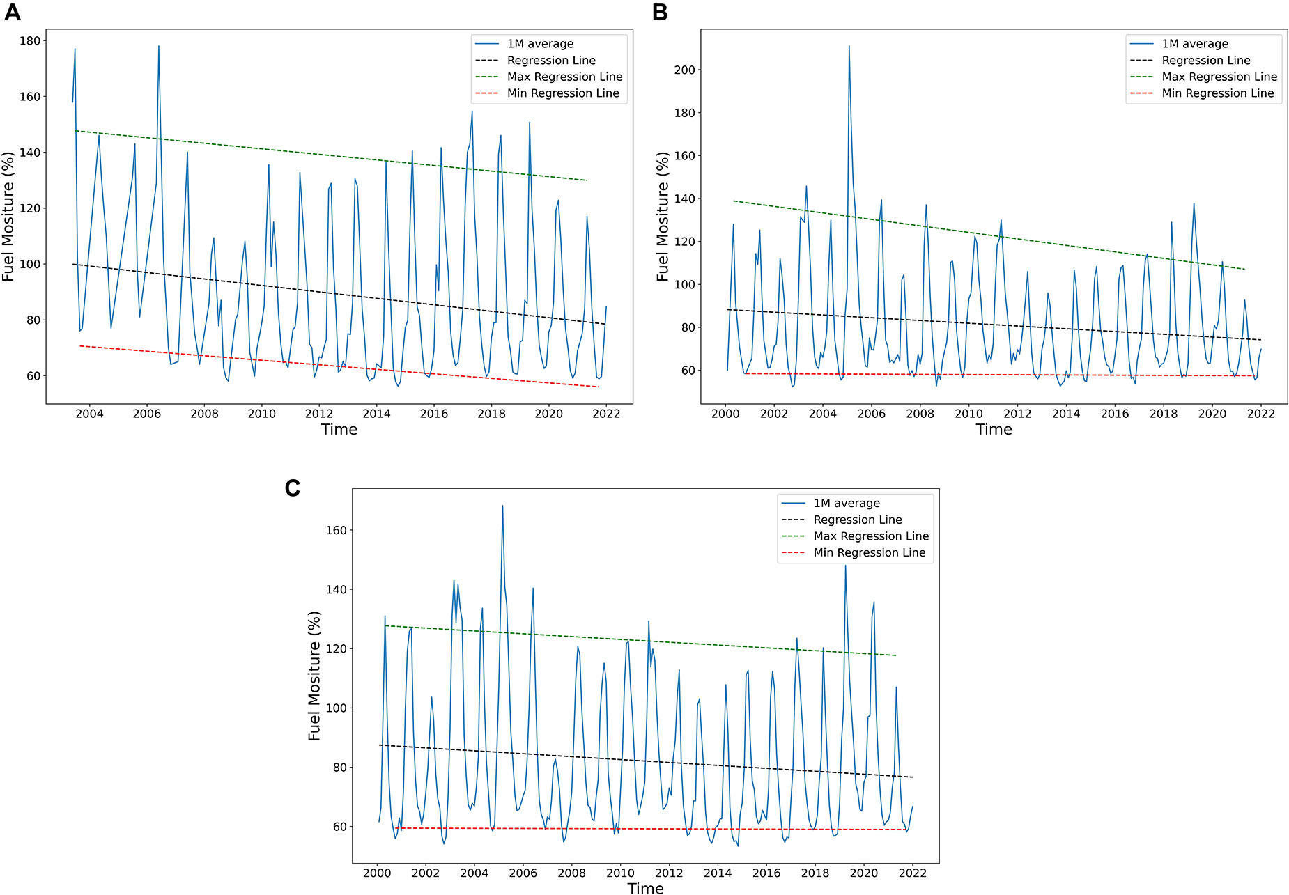
Figure 4. The general (annual average) (black dashed line), maximum (green dashed line), and minimum (red dashed line) LFMC trends for the (A) Bay Area, (B) Central Coast, and (C) South Coast regions. The differences in the time ranges stem from the length of the data record which varies across the regions.

FIGURE 5

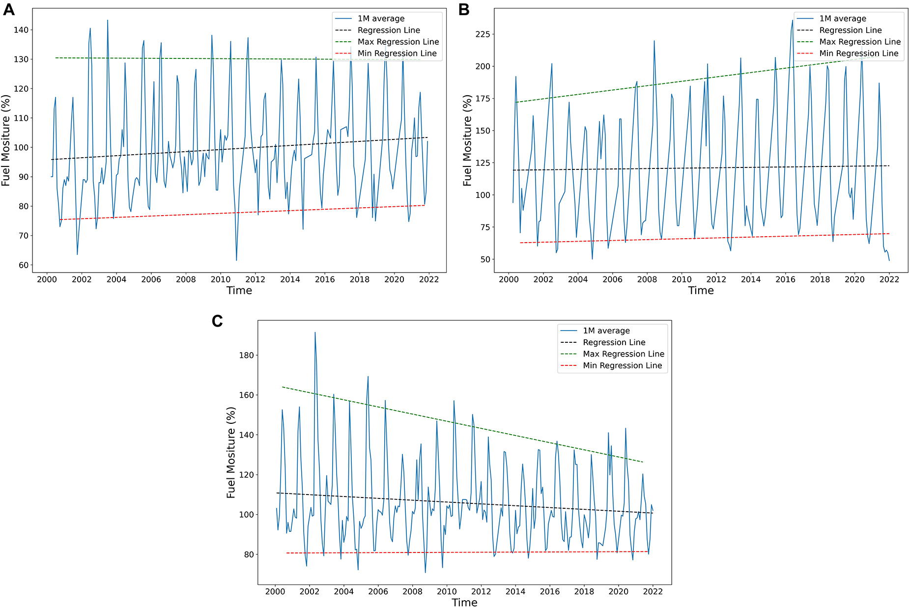
Figure 5. The general (annual average) (black dashed line), maximum (green dashed line), and minimum (red dashed line) LFMC trends for the (A) Klamath, (B) MODOC, and (C) Sierra Nevada regions. The differences in the time ranges stem from the length of the data record which varies across the regions.

FIGURE 6

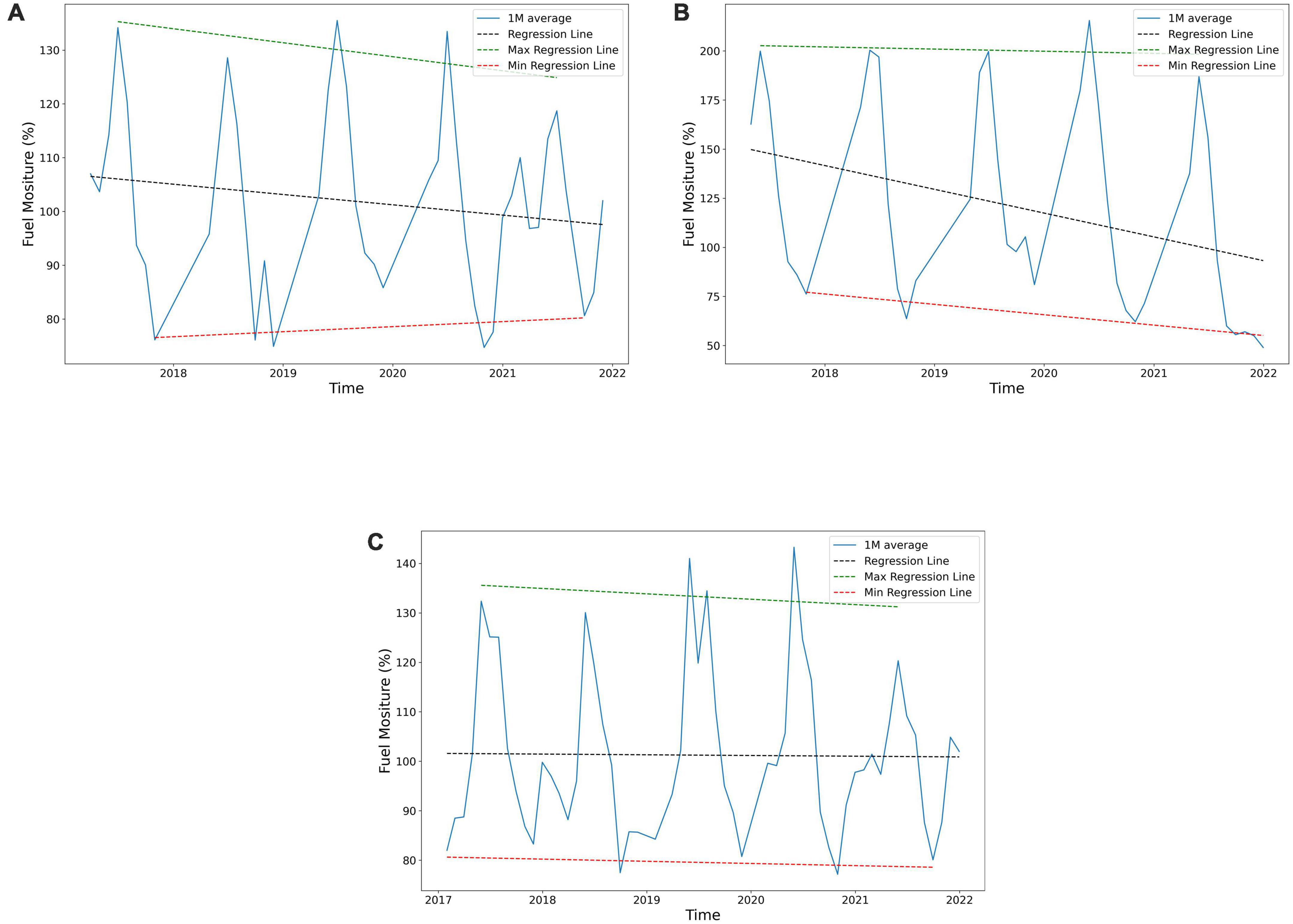
Figure 6. The general (annual average) (black dashed line), maximum (green dashed line), and minimum (red dashed line) LFMC trends for the (A) Bay Area, (B) Central Coast, and (C) South Coast regions from 2017–2021.

FIGURE 7

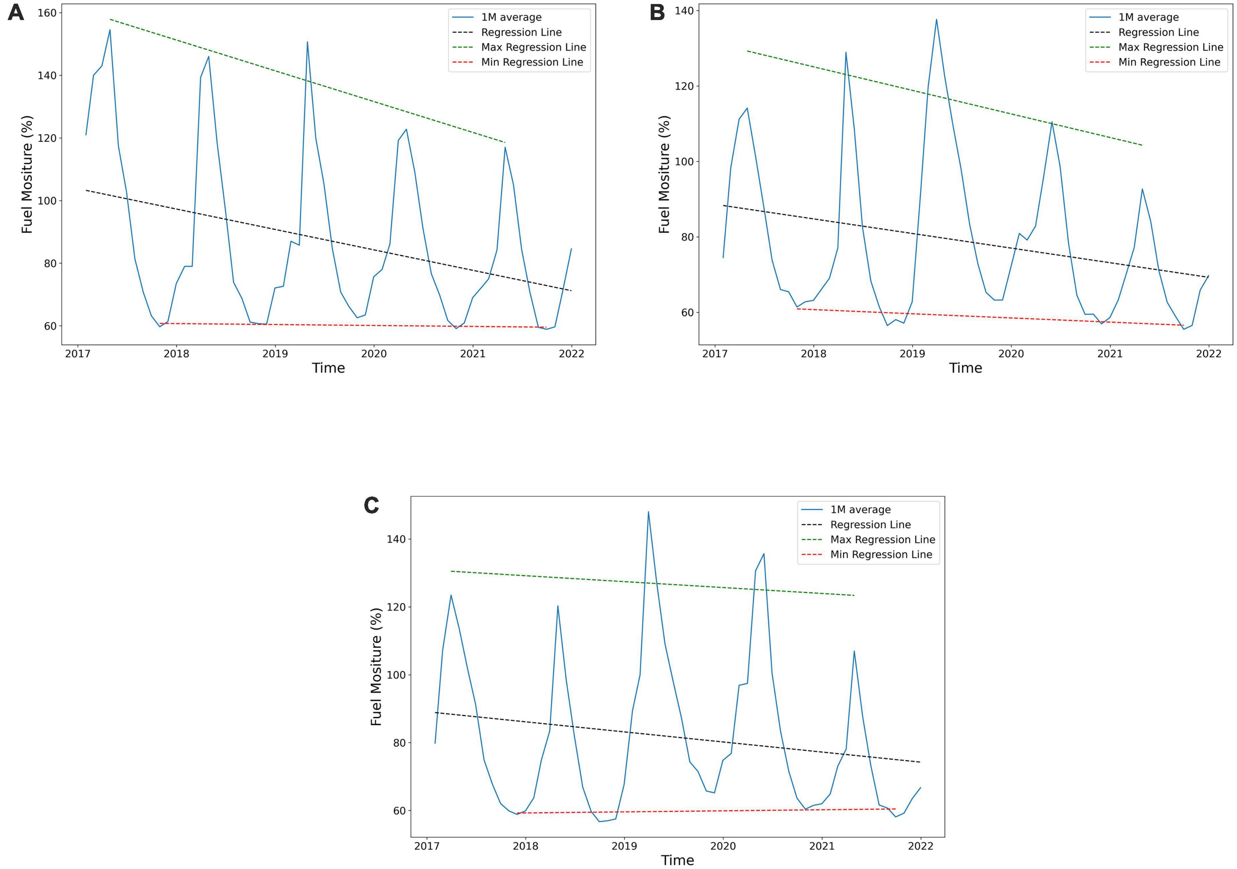
Figure 7. The general (annual average) (black dashed line), maximum (green dashed line), and minimum (red dashed line) LFMC trends for the (A) Klamath, (B) MODOC, and (C) Sierra Nevada regions from 2017–2021.

2.4. Drought impact on LFMC

To examine the impact of water deficit on LFMC variability, data from the Drought Monitor were used. The Drought Monitor, a product jointly generated by the National Drought Mitigation Center (NDMC) at the University of Nebraska-Lincoln, the National Oceanic and Atmospheric Administration (NOAA), and the U.S. Department of Agriculture (USDA), provides weekly drought estimates across the United States. There are 5 drought variables, each representing different drought levels on a given week: D0, D1, D2, D3, and D4. These levels are based on varying outputs from Palmer Drought Severity Index, CPC Soil Moisture Model, USGS Weekly Streamflow, Standardized Precipitation Index, and Objective Drought Indicator Blends. Further explanations of how these drought variables were created can be found at the Drought Monitor (n.d.).

For this study, California county drought data were used. The counties were grouped into the 6 regions listed above (Section “2.2. Regions”) and were used to extract and average the data from the drought dataset. The Drought Severity Metric (DSM) was created to determine the overall weekly drought severity for each region (Eq. 1), which can be correlated with LFMC observations. The metric was created as a weighted average, giving each drought level equal weight, to reduce the weekly 5 drought variables into a single value. Each drought variable [shown in Eq. 1 as Data (D0-D4)] is valued between 0–100%. With that in mind, the metric value ranges from 0–5, with 0 being no/slight drought conditions and 5 being the worst drought conditions. The metric was then applied to the drought dataset for each region. The integrated weekly drought values were then averaged across each year to create an annual drought severity value.

$DSM=\frac{Data\left[D0\right]+Data\left[D1\right]+Data\left[D2\right]+Data\left[D3\right]+Data\left[D4\right]}{100}(1)$

Once the annual drought severity value was found for each region from 2000–2021, the annual maximum and minimum LFMC values were gathered using the FMR. Using the drought severity metric as the colormap color reference, a heatmap was created to show the severity of drought each year, and the maximum, as well as minimum LFMC values, were superimposed over the drought conditions.

2.5. Burned area

We leverage the data from fuel moisture repository and the burned area derived from the Moderate Resolution Imaging Spectroradiometer (MODIS) to investigate the relationship between burnt area and the live fuel moisture. The MODIS Burned Area Product (MCD64A1) provides a gridded 500 m monthly dataset which was split into 6 subsets corresponding to the regions of interest. After sub-setting the data, our initial examination of the burned area data revealed a temporal lag in the data between the drying LFMC and the burned area. It has been documented that the MODIS Burned Area Product suffers from omission errors (non-reported burned pixels), commission errors (false alarms), overestimation (each 500 m cell was considered “burned” even if it didn’t completely burn), and burn date uncertainty that results in errors in burn date of over 15 days (Giglio et al., 2009; Ying et al., 2019). It has to be noted satellite fire observations are available at much higher frequency than the live fuel moisture data. The fuel moisture sampling is generally performed monthly, but the observations may be collected anytime within the month. As a consequence, when the fuel moisture observations are averaged monthly, observations at the very beginning of the month (representative of the previous month), or observations at the very end of the month (more representative of the following month) may skew the analysis by creating a time lag between the LFMC and fire activity.

To alleviate this time shift and the detection timing error, here we used the Last Day variable in the MODIS dataset, which provides the last day a pixel was detected as burning, and we averaged the fire data over a 2-month period. This averaging window smooths the burned area and makes it more consistent with low-frequency LFMC data. Once we organized the burned area data for each region, we utilized this data and the LFMC data in the contingency table presented in Table 2.

TABLE 2

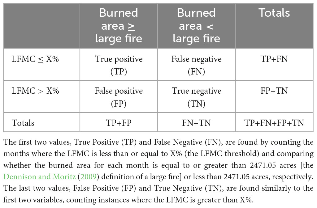
Table 2. Contingency table structure.

In the analyzed dataset, some regions had periods with burned area data but no LFMC data, so only periods where both were present were considered. We then ran the burned area and LFMC data through the contingency table, using an LFMC threshold of 79%, to obtain the TP, FN, FP, and TN values for each region. After that, we applied the output from the contingency table to Matthew’s Correlation Coefficient (MCC). The MCC was used to create a baseline correlation score as it combines all of the contingency table results into a single value, which ranges from −1 to 1, with −1 indicating a negative correlation between the predicted and observed values and 1 indicating a positive correlation between the predicted and observed values (Eq 2.). In the context of this study, a positive MCC supports the hypothesis of larger wildfires occurring when the LFMC drops below a certain threshold, while a negative MCC score rejects it, supporting an opposite hypothesis that large fires are associated with LFMC values above the threshold. A MCC value of 0 indicates a lack of relationship between the LFMC and burned area. The values of TP, FN, FP, TN, and MCC for each of the regions’ baselines are shown in Table 3.

$MCC=\frac{TP\cdot TN-FP\cdot FN}{\sqrt{\left(TP+FP\right)\cdot \left(TP+FN\right)\cdot \left(TN+FP\right)\cdot (TN+FN)}}(2)$

TABLE 3

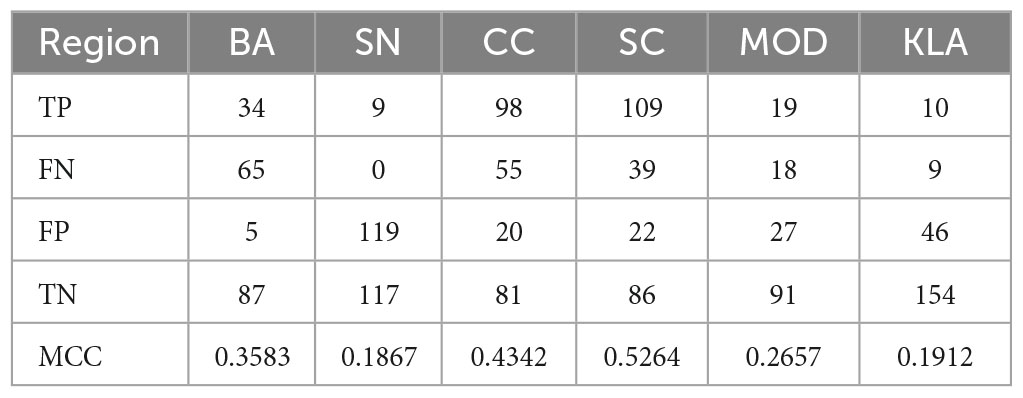
Table 3. Contingency table outputs and MCC score using the 79% LFMC threshold for each region.

To test the adequacy of the region specific baseline threshold, we repeated the process across each of the regions, but instead of using the predefined threshold of 79%, we examined different threshold values in the range between 30–100%. By investigating these possible thresholds, we identified optimal region-specific thresholds useful for indicating the potential for large fires by maximizing MCC. The results can be seen in Table 4.

TABLE 4

Table 4. Contingency table outputs, MCC score, and optimized LFMC threshold for each region.

We also examined the climatology of the fuels in each region along with the average burned area per month as well as the calculated LFMC threshold for each region. To achieve this, we found the monthly averaged burned area from our MODIS data for each region, similar to how we found the LFMC climatology, and plotted it together with the LFMC climatology and the calculated thresholds (Figures 2, 3).

3. Results and discussion

3.1. LFMC climatology

The analysis of the LFMC data indicated the variability in the dominant fuel types in the analyzed bioregions. For instance, Chamise, (Adenostoma Fasciculatum) was the dominant species for three regions (Bay Area, Central Coast, and the South Coast), in 2 regions the most sampled fuel was Manzanita, (Arctostaphylos manzanita), (Klamath, and the Sierra Nevada), while Sagebrush, Artemisia tridentata, was the predominant species in the Modoc region. It is clear by looking at Table 1 that shrubland plants are the dominant species sampled across all California regions, with Chamise and Manzanita being the two most common species. It must be noted that out of all the 6 analyzed regions, 2 (BA and MOD) had a relatively small number of observations given the sampling period and the size of the regions. Not only that, but the overall number of LFMC observations is relatively small given the number of sites as well as the temporal range of the data.

To streamline the analysis, the regions containing Chamise (Bay Area, Central Coast, and South Coast) were grouped together, while the regions characterized by Manzanita (Klamath and Sierra Nevada) were grouped separately. Additionally, the region featuring Sagebrush (Modoc) was included within the manzanita group. Starting with the Chamise regions, the typical monthly values and trends were analyzed and plotted in Figures 2, 4, respectively. These three regions span the California coastline, reaching from the far north to the southernmost tip. Being in relatively similar conditions, one would assume that the LFMC of the Chamise in these regions would also look similar to each other. This is not necessarily the case. The average LFMC maxima have an extreme range across the regions, ranging from about 105–125% with these maxima occurring around April. The average LFMC minima for these regions have a much smaller range, ranging from 58–60% and occur between September and October. Although there is a large range between the LFMC maxima across the regions, the drying period between when the maxima are reached to the time when the minima are reached is similar. Here we see that although the typical timing of the LFMC maxima and minima in chamise regions is similar, the maximum LFMC varies greatly, indicating variability in the duration of the drying periods.

Further examination of the LFMC trends in the Chamise regions shows a dire picture. Each of the regions has shown a downtrend in LFMC from 2000–2021. Specifically in the general trend and maximum trends (see Figure 4). This downtrend seen over the entire study period for these regions is minor relative to the downtrends over the last 5 years (2017–2021) as presented in Figure 6. While all the regions exhibit a downtrend in LFMC, the rates at which these downtrends are occurring are different, showing again the variation in LFMC even among the same fuel type. Before discussing these results in more detail, it is important to also analyze the Manzanita regions.

The Manzanita regions share less similarities between each other compared to the regions with Chamise, and have generally higher LFMC. To start, the maxima LFMC ranges from around 128–138% which is generally higher than chamise (105–125%). As shown in Figure 3, these maxima occur in May (for Sierra Nevada) and June (for Klamath) which is later than in Chamise. The minima, however, have a smaller spread, ranging only from 83–84%, and are reached around September and October similarly like in Chamise. Due to the Klamath region reaching its maximum LFMC in June, this region experiences a rapid drying period as it reaches its minimum LFMC in September/October compared to the Sierra Nevada which reaches its maximum in May. Variations in LFMC are significant between these two regions even though they contain the same fuel type. Quickly looking at the Modoc region, with Sagebrush as the dominant fuel, the maximum LFMC reaches around 177% in May and drops to its minimum of around 74% in September. In Figure 3B it can be seen that during December, the LFMC drops to around 50%, but observations during wet periods are sparse and this may be a single observation for that month.

Moving forward to the trends, we see a different picture in Manzanita than in the Chamise regions. Aside from the Sierra Nevada region which also has a downtrend in LFMC, similar to the Chamise regions, the Klamath and Modoc regions experienced an uptrend. Both are located in mountainous, heavily forested areas in the northern part of California. Due to their location and typical climatological trends in Northern California, these regions may experience more moisture. This likely causes these regions to have an uptrend in LFMC as compared to the more Southern ones (Bay Area, Sierra Nevada, Central Coast, and South Coast) which may experience more aridity. Although these regions have an uptrend, all of the Manzanita regions have a significant downtrend in LFMC over the last 5 years (2017–2021) (Figure 7), similar to the Chamise regions.

When looking at the overall trends of the regions, two of the six regions saw an uptrend and the rest saw a downtrend in LFMC. Although there were two regions with an uptrend, on average, altogether the regions experienced a general decrease of 9.58% in LFMC. The annual maxima decreased by 17.02% and the annual minima decreased by 9.18%. This downtrend is even more prevalent when looking at the last 5 years (2017–2021) (Figure 7). The average decrease across all of the regions in the last 5 years was 17.19%, with the annual maxima decrease of 13.93% and the annual minima decrease of 7.39%.

To extend our trend analysis we also ran the Mann-Kendall Test on the monthly averaged LFMC for each region from 2000–2021 (see Supplementary Table 4 in the Appendix). The Tau values presented there indicate trends consistent with the results from the linear regression test discussed above. The only difference was observed in Modoc region where linear regression showed a slightly positive trend, while Mann-Kendall test indicated a trend that is slightly negative.

Given the correlation between LFMC and wildfire development, this massive reduction in LFMC over the last 5 years appears to be a large factor in the larger fire developments recently seen throughout California. Considering the influential role of drought on live fuel moisture, the subsequent sections examine its significance in establishing possible associations between drought conditions, LFMC, and fire activity.

3.2. Drought

Most of the observed regions experienced similar drought periods from 2000–2021 as shown in Figure 8. During this time there are three distinct drought periods across California: between 2007–2009, 2012–2016, and 2020–2021. Even though there are evident drought periods across the state, some of the regions experienced more severe/less severe drought conditions than others. An example of this can be seen between the Klamath and Sierra Nevada regions in 2007. Manzanita is the predominant fuel type in both of these regions. The Klamath region entered slight drought conditions whereas the Sierra Nevada region saw moderate drought conditions compared to the prior year. These variations in the drought conditions across all of the regions shows strong evidence that drought does play a key role in the variability of LFMC, even among the same fuel types, and confirms why studies like Nolan et al. (2020) looked into the connections between drought and LFMC.

FIGURE 8

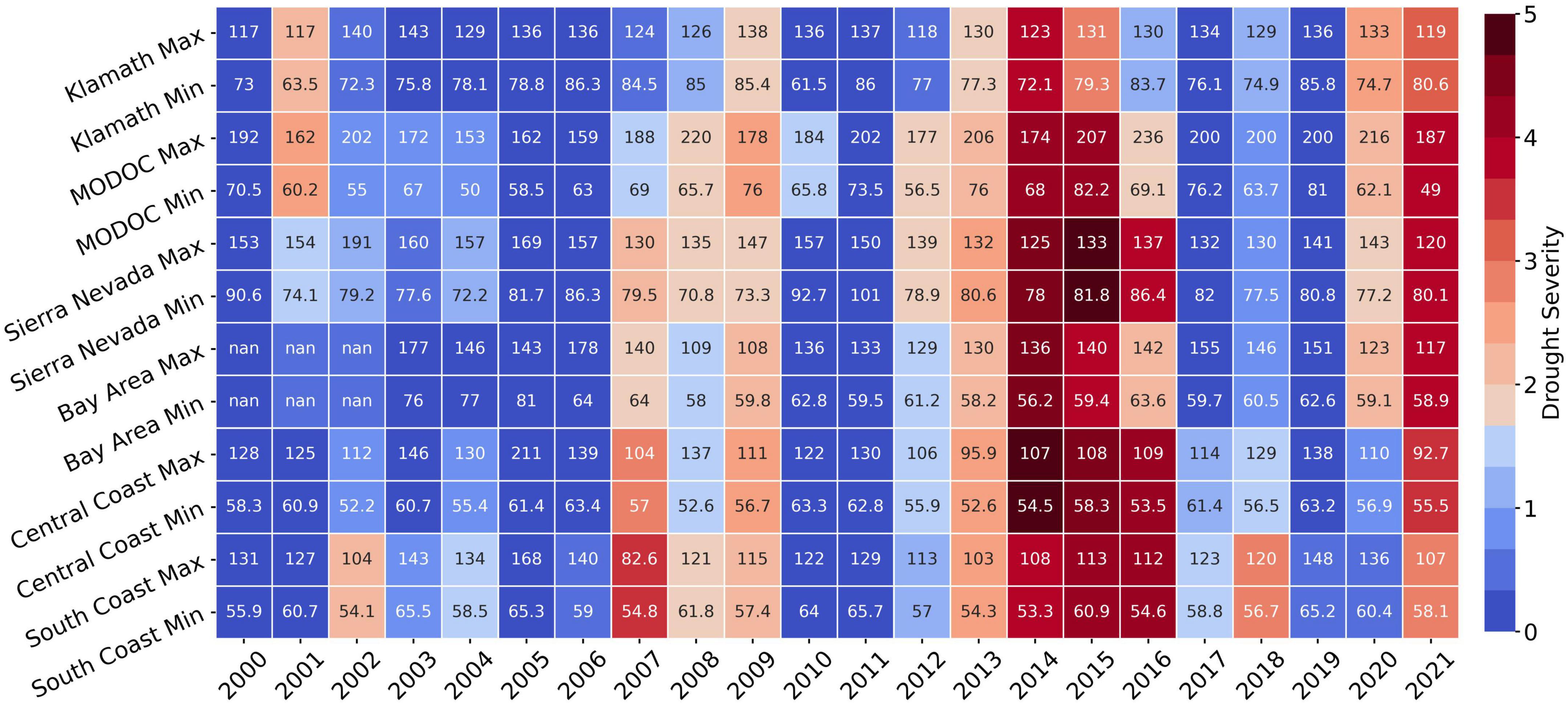
Figure 8. Heatmap displaying drought severity (ranging from dark blue to dark red indicating little/np drought to extreme drought, respectively). Every 2 rows show one region’s annual average maximum and minimum LFMC values as well as the drought conditions from 2000–2021. The x-axis represents each year, and the y-axis shows which region and what values (maximum or minimum) from a given region are observed.

Before delving into the drought and LFMC comparison, a few limitations of this study have to be pointed out. The first limitation is that even though drought data were available from the year 2000 to 2014, a limited amount of LFMC observations during that time made the presented analysis less robust in the early years. The second limitation is that there is only one non-drought period following 2014, which made it difficult to find any climatological patterns.

As drought conditions worsened, it was originally hypothesized that the maximum and minimum LFMC would decrease and vice versa when drought conditions lessened. As suspected, it was found that whenever a region entered a drought period, the LFMC usually dropped relative to the previous year and when drought conditions eased, the LFMC increased from the prior year. However, one interesting observation was how the LFMC behaved during extended drought periods, typically of two or more years. When a given drought period in a region extended for a few years, the maximum and minimum LFMC would stabilize and sometimes even rise during the following years. This can be observed in Figure 8 in the thirteenth row (South Coast Max) from 2013–2017. In 2013, the region entered a drought period and the max LFMC was 103%, down from the previous year of 113%. The following year, the drought conditions continued but the max LFMC rose to 108%. This trend of increasing and stabilization of the LFMC occurred until 2017 when drought conditions lessened and the LFMC rose from 112% in 2016 to 123% in 2017. This could be due to the plant’s physiology, allowing the plant to adapt to drought conditions. Another potential reason why we may observe this stabilization of the LFMC during extended drought periods may have to do with the way LFMC was defined. The equation for FMC utilizes the wet and dry mass of a plant. During periods when the plants are under high water stress, not only do they have a limited water supply, but they can potentially reduce their dry mass to offset water loss. Therefore, during extended drought periods, a decrease in the dry mass even with identical amount of water may lead to higher moisture content.

However, the most recent drought period from 2020–2021 shows that the maximum LFMC is not responding as expected. The regions that entered drought periods in 2020 saw a drop in LFMC as expected. Going into 2021, each of those regions experienced another drop in LFMC. Based on previous drought periods, there should have been some sort of stabilization or increase in LFMC. Not only is the LFMC during this period not indicating this behavior as it did in previous drought years, but the values approached or reached their lowest levels ever recorded. This may indicate that combination of the consecutive droughts led the LFMC to a breaking point after which the LFMC recovery observed earlier was not possible.

The analysis presented above clearly indicates differences in the LFMC and drought conditions across the analyzed regions. In order to investigate the possible connection between the variability in the LFMC and fire activity, the next section compares MODIS-derived burned area to the observed fluctuations in fuel moisture.

3.3. Burned area

Williams et al. (2019) found that fire activity in California had increased dramatically over the past decade, in part due to a reduction in LFMC. In order to conduct our investigation into the connection between LFMC and fire activity, we utilized the Dennison and Moritz (2009) definitions of large fires and their LFMC threshold to compare our LFMC observations and MODIS data. Tables 3, 4 show the Dennison and Moritz (2009) baseline threshold and the calculated thresholds for each region, respectively. The baseline MCC scores are relatively high for the Central Coast and South Coast and low for the other regions (low MCC values denote a weak relationship between the burned area and LFMC threshold and while high values indicate a stronger relationship). Upon iterating through the various potential thresholds for each region, more optimal thresholds were found for the regions resulting in a significant increase in regional MCC. All of the new thresholds ranged between 70 and 98%. The thresholds for regions that contained Chamise (Bay Area, Central Coast, and South Coast) were within 9% of the ones published by Dennison and Moritz (2009). The regions with Manzanita (Sierra Nevada and Klamath) had thresholds that differed by up to 13%, and the regions containing other fuel types (Modoc) saw up to a 19% difference compared to Dennison and Moritz (2009).

Although most of the locally optimized thresholds differed from the 79% threshold, the regions with Chamise fuels came out to be very close to it, and our estimates for the South Coast (which included the region the original study observed) matched exactly 79% building confidence in our methodology for finding optimal LFMC thresholds. It also appears that the same fuel types share similar LFMC thresholds across different regions, even with varying LFMC.

The climatology of LFMC in each region and its monthly average burned area relative to our LFMC thresholds are shown in Figures 2, 3. In these regions, on average, when the LFMC drops below the LFMC threshold, larger burned areas occur. However, there are outliers such as in the Sierra Nevada region during August when the LFMC is higher than the threshold and larger fires were occurring. One possible reason for this could be the impact of tree mortality due to drought and bark beetles (Restaino et al., 2019) which could lead to a high number of fire occurrences and reduce the importance of LFMC in the context of fire occurrences compared to dead fuels.

There were also some differences in the thresholds between the regions with Chamise and Manzanita. One of these differences can be observed in the period when the LFMC in each region dropped below their optimal threshold (Figures 2, 3). When the LFMC drops below the threshold, there tends to be a spike (around 15,000+ acres) in the burned area in each region. Looking at the regions with Chamise, the Bay Area experienced 4 months where the LFMC dropped below its optimal threshold and saw a burned area of around 15,000+ acres, 8 months in the Central Coast, and 7 months in the South Coast. Then, in the regions with Manzanita, we see the Klamath region below the threshold for about 3 months and 2 months in the Sierra Nevada region. The annual LFMC maxima and minima data may show why this has occurred. The regions with Chamise all have minima around 60% a year while their LFMC thresholds are about 10–22% higher whereas the regions with Manzanita have minima around 84% with their LFMC thresholds being about 4–8% higher. This increasing gap between the minimum LFMC and the optimal threshold indicates a longer period where we can see a potential increase in fire occurrences and an increase in the likelihood for larger fires to occur. The gap also indicates that the differences in the fuels between the regions lead to differences in the LFMC thresholds and therefore, varying burned area activity as shown in Figures 2, 3.

4. Conclusion

This paper describes the climatology of LFMC and how its changes correlate to wildfire activity in California. A repository was created that gathers data from the NFMD, stores it in a compact and organized way on a local machine, and allows users to easily query the data by regions, dates, and fuel types. The repository also provides basic plotting functionality that enables generation of fuel moisture time series, and box plots, which can be used to view the data before saving them to a file on the user’s local machine.

The analysis of the LFMC seasonality indicates that the timing of the maxima and minima vary by fuel type. Although the Chamise and Manzanita fuels tend to reach their minima at the same time (September/October) their maxima occur at different times (in April and May/June, respectively). Also, the peak and minimum LFMC values for Chamise were about 20% lower than for Manzanita. Aside from the differences between the fuel types, significant regional differences were observed even with the same fuel type. Depending on the location, Chamise LFMC varied by as much as 20% in maxima, while all the values for Manzanita were within just 10% regardless of the region.

Despite the strong region-to-region variability, the presented analysis indicates a downtrend across California with an exception in the Northernmost regions which have a slight uptrend. Across all the regions, there has been about a 9.58% average decrease in LFMC from 2000–2021. The annual maximum LFMC decreased by about 17.02% and the annual minimum decreased by around 9.18%. In the last 5 years, the average decrease across all of the regions reached 17.19%, with the annual maximum decreased by 13.93% and the annual minimum by 7.39%. This decrease in LFMC over the last 5 years may be linked to the larger fire developments recently seen throughout California. To investigate the observed variability in LFMC, the LFMC was compared to drought data. This comparison indicates significant variability in drought conditions across the regions, as well as its importance in controlling the LFMC. Observational data suggest that during extended drought periods, the plants adapted to the drought conditions, maintaining or even increasing their moisture content from year to year. The variability in LFMC was also shown to correlate with wildfire growth. By comparing burn area and LFMC data, region-specific LFMC thresholds that can be used to indicate the large wildfire potential, have been identified.

Live fuel moisture content has been previously found to be a critical component to fire danger assessment as well as wildfire growth, and an important variable that can be used to better understand fire danger and fire behavior. This study outlines temporal and spatial LFMC variability, investigates trends, as well as demonstrates links between LFMC, drought conditions, and fire activity.

Data availability statement

The raw data supporting the conclusions of this article will be made available by the authors, without undue reservation.

Author contributions

JD wrote the manuscript and led the analysis of the data. AK and CC conceived the original study design. AK managed the study execution. AF collected the datasets and aided in the development of the methodology. All authors contributed to the article and approved the submitted version.

Funding

This study was partially funded by the San Diego Gas and Electric Q201364 (project # 5660058288), USFS agreements # 21-CS-11221637-215 and 22-CR-11221633-027 as well as LLNL contracts B650931 and B655140. This study utilized live fuel moisture observations conducted by the SJSU Wildfire Interdisciplinary Research Center.

Conflict of interest

The authors declare that the research was conducted in the absence of any commercial or financial relationships that could be construed as a potential conflict of interest.

Publisher’s note

All claims expressed in this article are solely those of the authors and do not necessarily represent those of their affiliated organizations, or those of the publisher, the editors and the reviewers. Any product that may be evaluated in this article, or claim that may be made by its manufacturer, is not guaranteed or endorsed by the publisher.

Supplementary material

The Supplementary Material for this article can be found online at: https://www.frontiersin.org/articles/10.3389/ffgc.2023.1203536/full#supplementary-material

References

Bowers, C. (2018). The diablo winds of Northern California: Climatology and numerical simulations. Dissertation. San Jose, CA: San Jose State University.

Google Scholar

Chatelon, F. J., Balbi, J. H., Cruz, M. G., Morvan, D., Rossi, J. L., Awad, C., et al. (2022). Extension of the Balbi fire spread model to include the field scale conditions of shrubland fires. Int. J. Wildland Fire 31, 176–192. doi: 10.1071/wf21082

CrossRef Full Text | Google Scholar

Chuvieco, E., González, I., Verdú, F. R., Aguado, I., and Yebra, M. (2009). Prediction of fire occurrence from live fuel moisture content measurements in a Mediterranean ecosystem. Int. J. Wildland Fire 18:430. doi: 10.1071/wf08020

CrossRef Full Text | Google Scholar

Crutzen, P. J., and Andreae, M. O. (1990). Biomass burning in the tropics: Impact on atmospheric chemistry and biogeochemical cycles. Science 250, 1669–1678. doi: 10.1126/science.250.4988.1669

PubMed Abstract | CrossRef Full Text | Google Scholar

Danson, F. M., and Bowyer, P. (2004). Estimating live fuel moisture content from remotely sensed reflectance. Remote Sens. Environ. 92, 309–321. doi: 10.1016/j.rse.2004.03.017

CrossRef Full Text | Google Scholar

Deák, B., Valkó, O., Török, P., Végvári, Z., Hartel, T., Schmotzer, A., et al. (2014). Grassland fires in Hungary – experiences of nature conservationists on the effects of fire on Biodiversity. Appl. Ecol. Environ. Res. 12, 267–283. doi: 10.15666/AEER/1201_267283

CrossRef Full Text | Google Scholar

Delgado, E. D. (2009). “The National Fuel Moisture Database (NFMD) and the need for national fuels sampling and data standards,” in Paper presented at the Eighth symposium on fire and forest meteorology, Savannah, GA.

Google Scholar

Dennison, P. E., and Moritz, M. A. (2009). Critical live fuel moisture in chaparral ecosystems: A threshold for fire activity and its relationship to antecedent precipitation. Int. J. Wildland Fire 18:1021. doi: 10.1071/wf08055

CrossRef Full Text | Google Scholar

Dennison, P. E., Roberts, D. A., Thorgusen, S. R., Regelbrugge, J. C., Weise, D. R., and Lee, C. T. (2003). Modeling seasonal changes in live fuel moisture and equivalent water thickness using a cumulative water balance index. Remote Sens. Environ. 88, 442–452. doi: 10.1016/j.rse.2003.08.015

CrossRef Full Text | Google Scholar

Dimitrakopoulos, A. P., and Papaioannou, K. K. (2001). Flammability assessment of mediterranean forest fuels. Fire Technol. 37, 143–152. doi: 10.1023/a:1011641601076

CrossRef Full Text | Google Scholar

Drought Monitor (n.d.). Drought classification | U.S. Drought Monitor. Available online at: https://droughtmonitor.unl.edu/About/AbouttheData/DroughtClassification.aspx (accessed May 30, 2023).

Google Scholar

Giglio, L., Loboda, T., Roy, D. P., Quayle, B., and Justice, C. O. (2009). An active-fire based burned area mapping algorithm for the MODIS sensor. Remote Sens. Environ. 113, 408–420. doi: 10.1016/j.rse.2008.10.006

CrossRef Full Text | Google Scholar

Hamed, K. H., and Ramachandra Rao, A. (1998). A modified Mann-Kendall trend test for autocorrelated data. J. Hydrol. 204, 182–196. doi: 10.1016/s0022-1694(97)00125-x

CrossRef Full Text | Google Scholar

Lelieveld, J., Evans, J. S., Fnais, M., Giannadaki, D., and Pozzer, A. (2015). The contribution of outdoor air pollution sources to premature mortality on a global scale. Nature 525, 367–371. doi: 10.1038/nature15371

PubMed Abstract | CrossRef Full Text | Google Scholar

Mandel, J., Beezley, J. D., Kochanski, A. K., Kondratenko, V. Y., and Kim, M. (2012). Assimilation of perimeter data and coupling with fuel moisture in a wildland fire–atmosphere DDDAS. Procedia Comput. Sci. 9, 1100–1109. doi: 10.1016/j.procs.2012.04.119

CrossRef Full Text | Google Scholar

Matthews, S. (2014). Dead fuel moisture research: 1991–2012. Int. J. Wildland Fire 23, 78–92. doi: 10.1071/wf13005

CrossRef Full Text | Google Scholar

McCandless, T. C., Kosovic, B., and Petzke, W. (2020). Enhancing wildfire spread modelling by building a gridded fuel moisture content product with machine learning. Mach. Learn. Sci. Technol. 1, 1–12. doi: 10.1088/2632-2153/aba480

CrossRef Full Text | Google Scholar

Nelson, R. M. Jr. (2000). Prediction of diurnal change in 10-h fuel stick moisture content. Can. J. For. Res. 30, 1071–1087. doi: 10.1139/x00-032

CrossRef Full Text | Google Scholar

Nolan, R. H., Blackman, C. J., de Dios, V. R., Choat, B., Medlyn, B. E., Li, X., et al. (2020). Linking forest flammability and plant vulnerability to drought. Forests 11:779. doi: 10.3390/f11070779

CrossRef Full Text | Google Scholar

Nolan, R. H., Boer, M., Dios Resco De, V., Caccamo, G., and Bradstock, R. (2016). Large-scale, dynamic transformations in fuel moisture drive wildfire activity across southeastern Australia. Geophys. Res. Lett. 43, 4229–4238. doi: 10.1002/2016gl068614

CrossRef Full Text | Google Scholar

Nolan, R. H., Hedo, J., Arteaga, C., Sugai, T., and Resco de Dios, V. (2018). Physiological drought responses improve predictions of live fuel moisture dynamics in a Mediterranean Forest. Agric. For. Meteorol. 263, 417–427. doi: 10.1016/j.agrformet.2018.09.011

CrossRef Full Text | Google Scholar

Pausas, J. G., and Keeley, J. E. (2019). Wildfires as an ecosystem service. Front. Ecol. Environ. 17:289–295. doi: 10.1002/fee.2044

CrossRef Full Text | Google Scholar

Pellizzaro, G., Cesaraccio, C., Duce, P., Ventura, A., and Zara, P. (2007). Relationships between seasonal patterns of live fuel moisture and meteorological drought indices for Mediterranean shrubland species. Int. J. Wildland Fire 16:232. doi: 10.1071/wf06081

CrossRef Full Text | Google Scholar

Pollet, J., and Brown, A. (2007). Fuel moisture sampling guide. Missoula, MT: United States Department of Agriculture, Forest Service, Missoula Technology and Development Center: Technology and Development Program.

Google Scholar

Qi, Y., Dennison, P. E., Spencer, J., and Riaño, D. (2012). Monitoring live fuel moisture using soil moisture and remote sensing proxies. Fire Ecol. 8, 71–87. doi: 10.4996/fireecology.0803071

CrossRef Full Text | Google Scholar

Rao, K., Williams, A. P., Flefil, J. F., and Konings, A. G. (2020). Sar-enhanced mapping of live fuel moisture content. Remote Sens. Environ. 245, 1–12. doi: 10.1016/j.rse.2020.111797

CrossRef Full Text | Google Scholar

Restaino, C., Young, D. J. N., Estes, B., Gross, S., Wuenschel, A., Meyer, M., et al. (2019). Forest structure and climate mediate drought-induced tree mortality in forests of the Sierra Nevada, USA. Ecol. Appl. 29:e01902. doi: 10.1002/eap.1902

PubMed Abstract | CrossRef Full Text | Google Scholar

Rollins, M. G., Keane, R. E., and Parsons, R. A. (2004). Mapping fuels and fire regimes using remote sensing, ecosystem simulation, and Gradient Modeling. Ecol. Appl. 14, 75–95. doi: 10.1890/02-5145

CrossRef Full Text | Google Scholar

Rothermel, R. C. (1972). A mathematical model for predicting fire spread in wildland fuels. Ogden, UT: Intermountain Forest & Range Experiment Station, Forest Service, U.S. Dept. of Agriculture.

Google Scholar

Ruffault, J., Martin-StPaul, N., Pimont, F., and Dupuy, J. L. (2018). How well do meteorological drought indices predict live fuel moisture content (LFMC)? an assessment for wildfire research and operations in Mediterranean ecosystems. Agric. For. Meteorol. 262, 391–401. doi: 10.1016/j.agrformet.2018.07.031

CrossRef Full Text | Google Scholar

The Editors of Encyclopaedia Britannica (2015). Climatology | meteorology. Available online at: https://www.britannica.com/science/climatology (accessed May 30, 2023).

Google Scholar

van der Molen, M. K., Dolman, A., Ciais, P., Eglin, T., Gobron, N., Law, B., et al. (2011). Drought and ecosystem carbon cycling. Agric. For. Meteorol. 151, 765–773. doi: 10.1016/j.agrformet.2011.01.018

CrossRef Full Text | Google Scholar

van Wagner, C. E. (1987). Development and Structure of the Canadian Forest Fire Weather Index System. Volume 35. Forestry Technical Report. Ontario: Canadian Forestry Service.

Google Scholar

Vejmelka, M., Kochanski, A. K., and Mandel, J. (2016). Data assimilation of dead fuel moisture observations from remote automated weather stations. Int. J. Wildland Fire 25, 558–568. doi: 10.1071/wf14085

CrossRef Full Text | Google Scholar

Viegas, D. X., Piñol, J., Viegas, M. T., and Ogaya, R. (2001). Estimating live fine fuels moisture content using meteorologically-based indices. Int. J. Wildland Fire 10:223. doi: 10.1071/wf01022

CrossRef Full Text | Google Scholar

Williams, A. P., Abatzoglou, J. T., Gershunov, A., Guzman-Morales, J., Bishop, D. A., Balch, J. K., et al. (2019). Observed impacts of anthropogenic climate change on wildfire in California. Earths Future 7, 892–910. doi: 10.1029/2019ef001210

CrossRef Full Text | Google Scholar

Yebra, M., Dennison, W., Chuvieco Salinero, E., Riaño, D., Zylstra, P., Hunt, E. R., et al. (2013). A global review of remote sensing of live fuel moisture content for fire danger assessment: Moving towards Operational Products. Remote Sens. Environ. 136, 455–468. doi: 10.1016/j.rse.2013.05.029

CrossRef Full Text | Google Scholar

Ying, L., Shen, Z., Yang, M., and Piao, S. (2019). Wildfire detection probability of MODIS fire products under the constraint of environmental factors: A study based on confirmed ground wildfire records’, Remote Sens. 11:3031. doi: 10.3390/rs11243031

CrossRef Full Text | Google Scholar