Allometric scaling and allocation patterns: Implications for predicting productivity across plant communities

As the application of allometry continues to expand, the variability in the allometry exponent has generated a great deal of debate in forest ecology. Some studies have reported counterintuitive values of the exponent, but the sources of such values have remained both unexplored and unexplained. Therefore, the objectives of our analyses were to: (1) uncover the global patterns of allometric variation in stem height with stem diameter, crown radius with stem diameter or stem height, crown depth with stem diameter, crown volume with stem diameter, crown depth with crown diameter, aboveground biomass with stem diameter or height, and belowground biomass with aboveground biomass; (2) assess variations in allometry parameters with taxonomic levels, climate zones, biomes and historical disturbance regimes; and (3) identify the sources of counterintuitive values of the allometry exponents. Here, we provide novel insights into the tight allometric co-variations between stem and crown dimensions and tree biomass. We also show a striking similarity in scaling across climate zones, biomes and disturbance regimes consistent with the allometry constraint hypothesis. We show that the central tendency of the exponent is toward 2/3 for the scaling of stem height with diameter, crown dimensions with stem diameter and height, 5/2–8/3 for the scaling of aboveground biomass with stem diameter, and 1 for the scaling of belowground biomass with aboveground biomass. This is indicative of an integrated growth regulation acting in tandem on growth in stem diameter, height, crown dimensions and biomass allocation. We also demonstrate that counterintuitive values of the exponent arise as artifacts of small sample sizes (N < 60), measurement errors, sampling biases and inappropriate regression techniques. We strongly recommend the use of larger sample sizes (N > 60) and representative samples of the target population when testing hypothesis about allometric variation. We also caution against conflation of statistical artifacts with violations of theoretical predictions.

Introduction

Variety of biological systems display striking regularities, which often take the form of power laws characterized by scale invariance and universality (Enquist et al., 1999; Enquist and Niklas, 2001; Brown et al., 2002; Marquet et al., 2005). Allometric scaling of biological traits with the body size of organisms is one such example (Enquist et al., 1999; Brown et al., 2002). As originally defined by Huxley and Teissier (1936), allometry designates relative changes in one dimension (ΔY/Y) in relation to a second dimension (ΔX/X), usually the body size of an organism. In order to avoid confusion, Huxley and Teissier (1936) agreed to consistently use the term allometry and the conventional power law formula Y = αX^β.

Despite wide variations in their growth forms and life history characteristics, plants exhibit a striking regularity in allometric scaling in form and function with changes in body size (Enquist et al., 1999; Kerkhoff et al., 2005; Kerkhoff and Enquist, 2006). At the individual plant level, allometric constraint arises probably because the growth of the whole “trait complex” is under a common (integrated) growth regulation. A growing body of evidence also suggests that allometric constraints at an individual plant level have implications for the structure and dynamics of plant populations and ecosystems (Enquist et al., 2003; Kerkhoff et al., 2005; Kerkhoff and Enquist, 2006). As such, analysis of allometric scaling can help in identifying general principles that apply across a wide range of scales and levels of organizations (Marquet et al., 2005). Historically, disturbance regimes have shaped the development of specific adaptations in plants. For example, geoxylic life forms (underground trees) and thick, corky bark have evolved in response to frequent fires in savannas (Maurin et al., 2014). On the other hand, tropical rain forests are pyrophobic, and often do not have specific adaptations against fire. Forest disturbance regimes such as fire are changing in response to global environmental change (Sommerfeld et al., 2018). Therefore, analyses of allometric trajectories with the changing disturbance regimes can facilitate better understanding of the impacts of climate change or land use changes.

Analysis of allometric scaling can also facilitate our understanding of patterns of resource allocation in forests. Traditionally, allocation in plants has been conceptualized as a ratio-driven process (Weiner, 2004), which is at the core of the optimal partitioning theory (Qi et al., 2019). While this theory has been a cornerstone of many studies in plant ecology and evolution, its generality has been questioned, and more recently, the allometric biomass partitioning theory was proposed to predict how plants partition their metabolic production based on the constraints of body size (Niklas and Enquist, 2002; Weiner, 2004; Mccarthy and Enquist, 2007). Consequently, allometric models are now widely used for prediction of forest biomass and carbon stocks (Chave et al., 2014; Sileshi, 2014). More recently, the application of allometric models has gained increasing interest in remote sensing surveys of forest biomass at landscape and regional scales (Blanchard et al., 2016).

Allometric scaling is described by a power law function:

$Y=\alpha X^{\beta }\epsilon (1)$

or its linear form as:

$\text{ln(}Y)=\text{ln(}\alpha \text{)}+\beta \left(\text{ln}X\right)+\epsilon (2)$

where ln(α) is the intercept or offset of the line at ln(X) = 0 and β is the scaling exponent. Historically, β has been assumed to be constant and independent of α in Equation 1. Voje et al. (2013) have also shown that β may be difficult to change on short time scales. On the other hand, the interpretation of ln(α) has been less clear and its variability remains poorly understood.

As the application of allometry continues to expand, the variability in β has generated debates in forest ecology and biomass estimation literature (Sileshi, 2014). Allometric theories suggest that β tends to be a multiple of 1/3 or 1/4, and various hypotheses have been proposed to explain this pattern. An exponent of 1/3 is attributed to geometric scaling, i.e., area–volume ratios, whereas 1/4 is attributed to metabolic scaling imposed by transport of substances via branching networks (West et al., 1997, 2002; Enquist et al., 1999). Many studies (see Blanchard et al., 2016; Jucker et al., 2022) have opined that β is shaped by the environmental conditions of the stand, the individual trees, and by the diversity of tree communities. Others have argued that systematic departures from allometric scaling expectations may indicate particular disturbance processes (Kerkhoff and Enquist, 2006; Tredennick et al., 2013). Yet, in others it is said to vary with the taxonomic level of investigation. For example, the taxon-level effect hypothesis (Promislow et al., 1992) posits that β increases in both magnitude and statistical significance with increasing taxonomic level. Some studies have also reported counterintuitive values of β including negative values where positive values are expected. For example, for the crown depth to stem diameter allometry, Panzou et al. (2021) reported β values of −0.314 and −0.541 for Australian forests and American savannas, respectively, where β is expected to be a positive value falling between ½ and 1. For crown diameter to stem diameter allometry, Panzou et al. (2021) also reported β values of −0.087 for American forests, −0.125 for American savannas, −0.160 for Asian forests, −0.414 for Australian forests and −0.024 for Australian savanna where β is expected to be between ½ and 1. The sources of these counterintuitive values have remained both unexplored and unexplained.

Past studies in forest ecosystems have focussed on a single allometric relationships in specific sites or regions, for example, pan-tropical variability in biomass (Chave et al., 2014) or tree crown allometry (Shenkin et al., 2020; Panzou et al., 2021). In almost all studies, inferences were based on point estimates, and little is known about the distributions of allometry parameters. Understanding parameter distributions and the sources of variability is critical because these parameters hold the key for (1) accurate estimation of forest biomass and carbon stocks and (2) interpreting scaling relationships and how they vary with taxonomic lineages, biomes or disturbance regimes. Therefore, the objectives of the present analyses were to: (1) uncover the global patterns of allometric variation in stem height with stem diameter, crown radius with stem diameter or stem height, crown depth with stem diameter, crown volume with stem diameter, crown depth with crown diameter, aboveground biomass with stem diameter, and belowground biomass with aboveground biomass; (2) assess variations in allometry parameters with taxonomic levels, climate zones, biomes and historical disturbance regimes; and (3) identify the sources of counterintuitive values of the allometry exponents with a focus on statistical artifacts. A statistical artifact is a spurious finding that results from biases in the collection or analysis of data. Our key hypotheses are: (1) the allometry exponents systematically vary with taxonomic levels, divergence time and climate zones; (2) trees adapted to different biomes and disturbance regimes have different allometry exponents; (3) the tallest, hyper-emergent and short-statured tree species follow different allometric trajectories.

Materials and methods

Definitions, context, and scope of analysis

There are many fundamentally different approaches of defining and classifying climate zones and biomes. To reduce ambiguity in our analyses, we defined climate zones and biomes based on the current literature. We also identified and defined disturbance regimes within these well-defined climate zones and biomes.

Climate zones

For the definition of broad climate zones, we followed the FAO classification used for global forest resources assessment and reporting (FAO, 2012). This classification identifies five major zones, namely tropical, subtropical, temperate, boreal and polar zones (FAO, 2012). The tropical zone is within the area bounded by latitudes of 23.5° north and 23.5° south. The subtropical zone is applied to the two belts between the tropics (± 23.5°) and 35° north and south of the equator. Temperate zones fall in the latitudes of 35–50° north or south, and have well-defined seasons with a distinct winter. The boreal zone falls between 50 and 60° north. When testing our first hypothesis, we grouped the data according to the above classification based on the geographic coordinates of the study sites in the databases.

Terrestrial biomes

The biome is an important construct for organizing knowledge about terrestrial ecosystems, for examining diversity-productivity relationships, modeling historical distributions and shifts following climate change. We followed the IUCN Global Ecosystem Typology (Keith et al., 2022), which recognizes seven terrestrial biomes: (1) tropical-subtropical forests (T1); (2) temperate-boreal forests and woodlands (T2); (3) shrublands and shrubby woodlands (T3); (4) savannas and grasslands (T4); (5) deserts and semi-deserts (T5); (6) polar-alpine biomes (T6); and (7) intensive land-use (T7) biome. Each of these biomes is characterized by different ecosystem functional groups described in detail in Keith et al. (2022). The present analysis was limited to T1, T2, T3, and T4 as these have trees as the main or co-dominating components. Deserts and semi-deserts and polar-alpine biomes were deemed outside the scope of this analysis. Although some samples may have come from T7, it was difficult to assign them with confidence in the existing databases.

Disturbance agents and regimes

A disturbance regime is defined as the combination of disturbance agents and disturbance attributes that characterize a particular landscape or region (Burton et al., 2020). Disturbance interactions are an important part of the disturbance regime (Burton et al., 2020; Sturtevant and Fortin, 2021). The main disturbance agents in forest ecosystems consist of abiotic (e.g., fire, drought, wind, snow, and ice) and biotic (e.g., insects and pathogens) agents (Fischer et al., 2013; Stephens et al., 2013; Sturtevant and Fortin, 2021). According to a recent systematic review of disturbance interactions studies (Sturtevant and Fortin, 2021), the most frequently investigated natural disturbance agent was fire accounting for 65% of studies, followed by wind (38%), insects (37%), water imbalance (drought or flooding; 15%), mammalian browsing/grazing (10%), and mass movement including erosion, debris flows, landslides and avalanche (7%). Accordingly, the focus of this analysis was on fire, wind and insects as disturbance agents.

Fire is an important natural disturbance factor in many boreal forests, in savannas and high mountain dry-land ecosystems (Fischer et al., 2013). Low-severity fire regimes are typified by frequent low-intensity fires where surface fuels are charred or consumed while damage to overstory canopy is minimal (Giunta et al., 2016). In contrast, high-severity fire regimes are characterized by transitions from surface fuels into the crowns of trees, consuming a majority of overstory vegetation (Giunta et al., 2016). On the other hand, mega-fires are defined as fires covering an area exceeding 10,000 ha arising from single or multiple related ignition events (Stephens et al., 2013; Linley et al., 2022). Megafires occur in a range of biomes, but were most frequently reported in temperate-boreal forests and woodlands biomes (Linley et al., 2022). Species that grow in areas where low-severity fires occur frequently have special adaptations like thick bark (e.g., Pinus ponderosa), the ability to re-sprout after fire or store seeds on the tree until a fire occurs (Fischer et al., 2013) or geoxylic life forms in African savannas and Brazilian Cerrado (Maurin et al., 2014). Many savanna trees in Africa and eucalypts in Australian are dependent on fire for regeneration (Tng et al., 2012). These kinds of adaptations are missing in tropical rainforests and temperate forests, which do not naturally experience frequent fires (Tng et al., 2012; Fischer et al., 2013).

The primary effects of wind include damage and breakage to the tops of crowns, branches, uprooting, and snapping of trees (Giunta et al., 2016). Wind thrown trees can also create suitable habitat for bark beetles or increase the fuel load (Giunta et al., 2016). Wind damage risk increases with increase in height, and trees are known to adjust their growth pattern to their local wind environment (Jackson et al., 2021).

Remarkable among insects as disturbance agents are the bark beetle outbreaks causing large-scale transformations of forest landscapes in the northern hemisphere (Giunta et al., 2016; Hlásny et al., 2021). The European spruce bark beetle (Ips typographus) is the primary outbreak species in Europe causing as much as 8% of all tree mortality in Europe (Hlásny et al., 2021). Its damage to Norway spruce (Picea abies), its primary host, has been historically very high in the temperate latitudes than in boreal forests (Hlásny et al., 2021). A similar trend occurs in western Canada and the USA, where tree mortality due to the mountain pine beetle (Dendroctonus ponderosae) exceeds 28 million ha (Hlásny et al., 2021). In the USA, a rise in bark beetle activity since the early 1990s has occurred across a range of forest types (Giunta et al., 2016). The Douglas-fir beetle (Dendroctonus pseudotsugae) is the primary insect pest of interior Douglas-fir (Pseudotsuga menziesii) forests (Giunta et al., 2016). Another example of insect outbreaks, is aspen (Populus tremuloides) defoliation by forest tent caterpillars (Malacosoma disstria) in North America. For the present analysis, we focussed on tree species affected by the bark beetles and forest tent caterpillar outbreaks.

Allometries analyzed

For this analysis we chose allometric scaling between (1) stem height and stem diameter (H–D); (2) crown radius and stem diameter (CR–D) or stem height (CR–H); (3) crown diameter with stem diameter (CD–D), (4) crown depth with stem diameter (Cdep–D), (5) crown volume with stem diameter (Cvol-D); (6) crown depth with crown diameter (Cdep-CD); (7) aboveground biomass and stem diameter (A–D); and (8) belowground biomass and aboveground biomass (A-B).

Stem diameter, height, and crown dimensions

Understanding the relationship between H, D, and crown dimensions is fundamental in understanding the structure of forest stands, tree architecture and niche partitioning within a forest ecosystem and in the estimation of biomass and carbon storage (Hulshof et al., 2015; Blanchard et al., 2016). There are four allometric scaling hypotheses (geometric, stress, elastic, and metabolic) predicting different exponents for the H–D, CR–D, and CR–H scaling in trees (Table 1). Hypotheses based on geometric and dynamic growth arguments predict β to be 1 (Table 1), whereas the stress similarity hypothesis predicts β to be approximately ½. On the other hand, the elastic similarity hypothesis and the metabolic scaling theory (MST) predict β to be approximately 2/3 (West et al., 1997; Enquist et al., 1999). The elastic similarity hypothesis posits that for trees to resist buckling under their own mass, longer stems need to be proportionally thicker, and hence D should scale with H as the power of 2/3 (Osunkoya et al., 2007). It also posits that tree height is limited by either gravity or wind damage risk (Jackson et al., 2021). The MST assumes metabolic scaling under optimized tree architecture and resource transport (West et al., 1997).

TABLE 1

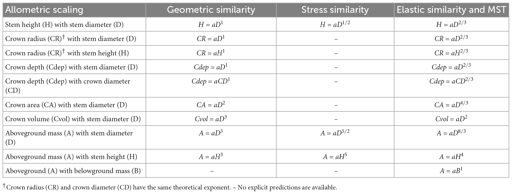
Table 1. Allometric scaling relationships among stem height, diameter at breast height, various crown dimensions and tree biomass and the theoretical expectations of the exponent of the geometric similarity, constant stress similarity, elastic similarity, and metabolic scaling theory (MST).

Height growth and crown development are known to be driven by competition for light; but why emergent and hyper-emergent trees continue to grow after escaping competition is not fully understood (Jackson et al., 2021). It is also not clear whether or not H–D, CR–D, and CR–H allometric trajectories differ between hyper-emergent and short-statured species. Therefore, we estimated the allometry parameters to understand their patterns of variation with taxonomic levels, biomes and disturbance regimes. In all instances, we used publicly available data from the Tallo database¹ built by Jucker et al. (2022). This database contains 498,838 standardized records of D, H, and CR for 5,163 tree species in 1,453 genera and 187 families from 61,856 globally distributed sites covering all the climate zones (Jucker et al., 2022). We conducted five different sets of analyses focussing on entries for which taxonomic identity was available in this database. We excluded entries without genus, family, and division names.

In the first set of analyses, we compared Gymnosperms and Angiosperms using the point estimates as well as the distributions of allometry parameters of the H–D, CR–D, and CR–H scaling (Figures 1, 2, Table 2, and Supplementary Table 1). We also compared the allometry exponents of selected families, genera and species within Gymnosperms and Angiosperms in order to understand patterns of variation with taxonomic levels and to test the validity of the “taxon-level effect” hypothesis (Supplementary Figures 1–4). For the family level comparisons, we chose the families Pinaceae within Gymnosperms and Fagaceae within Angiosperms because they had larger sample sizes compared to all other families. Then we chose the genera Pinus and Quercus because they had adequate sample sizes allowing further analyses at the species level. Within each of these two genera, first we estimated the H–D, CR–D, and CR–H allometry parameters for all species that had sample sizes of 10 or more. Then, we compared Pinus species with Quercus species in terms of the distribution of their H–D, CR–D, and CR–H exponents (Supplementary Figure 4). For further in-depth analyses, we chose Pinus sylvestris and Quercus rubra as they occurred in different climatic zones in the dataset. We produced point estimates and 95% confidence intervals (95% CI) of the allometry exponents of these species in the different climate zones (Table 2). We also made an in-depth analysis of Pinus sylvestris populations in temperate zones at the study level to identify factors associated with biases in the allometry exponents (Table 3). Here, bias is defined as the systematic discrepancy between an estimator and its expected values (Kelly, 2007) such as those in Table 1. Specifically, we examined effects of sample sizes, attenuation bias and sampling bias on the allometry exponent. Attenuation bias arises from measurement errors (Hutcheon et al., 2010) and is indicated by correlation coefficients (r) approaching zero where the true population correlation coefficient (ρ) is known to be large. It is also indicated by large discrepancies between ordinary least square (OLS) and reduced major axis (RMA) estimates of β (see section “Statistical analysis”).

FIGURE 1

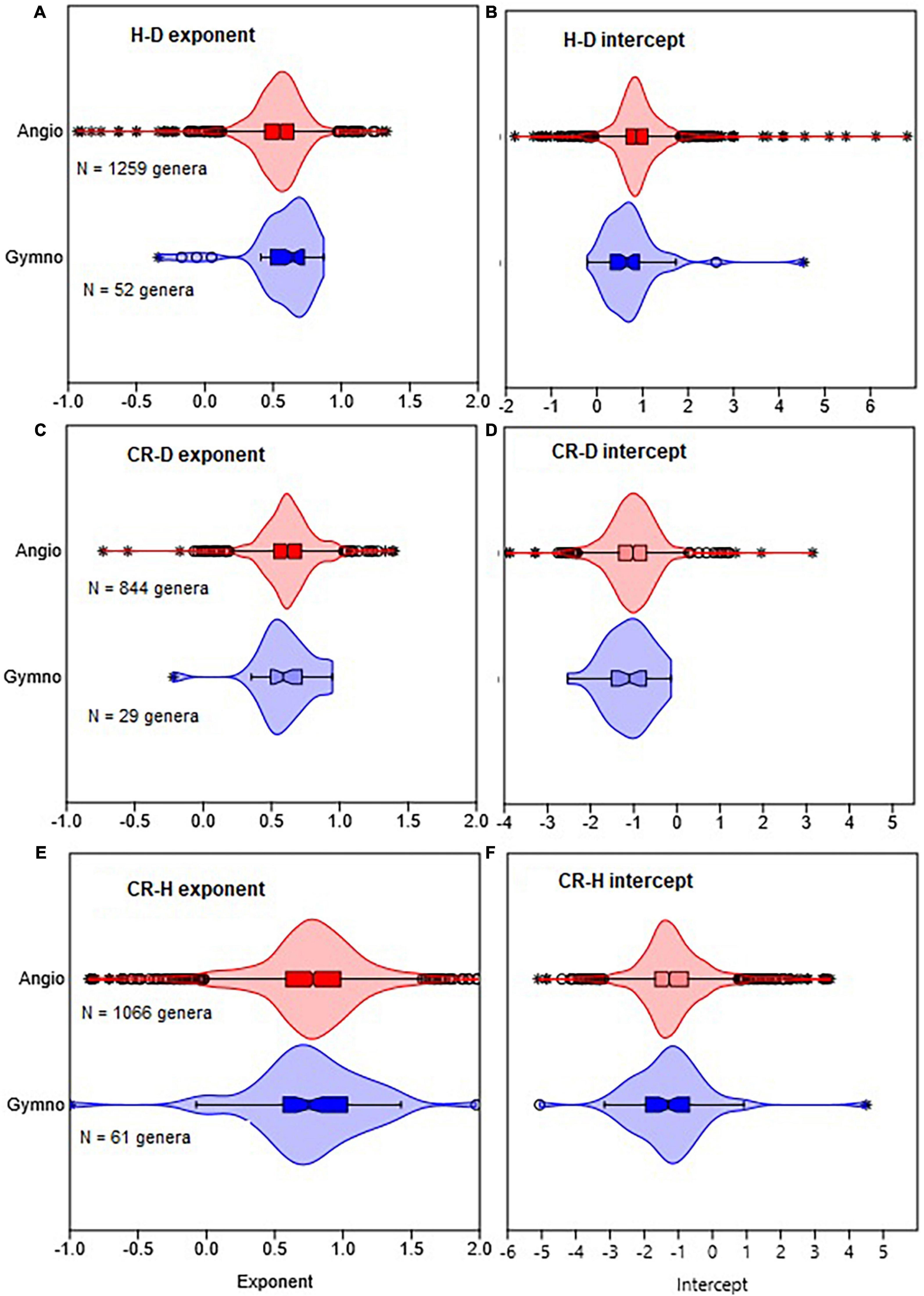
Figure 1. Comparison of gymnosperms with angiosperms in terms of the distribution of the allometric parameters of height with stem diameter (H–D), crown radius with stem diameter (CR–D), and crown radius with stem height (CR–H) scaling. The distributions of exponents are shown in (A,C,E), while intercepts are in (B,D,F). The box and whisker plots display the median and its 95% CI (notches), lower quartile, upper quartile, extreme values, and outliers (O and *). Distributions in all cases are based on OLS estimates of the parameters for each genus.

FIGURE 2

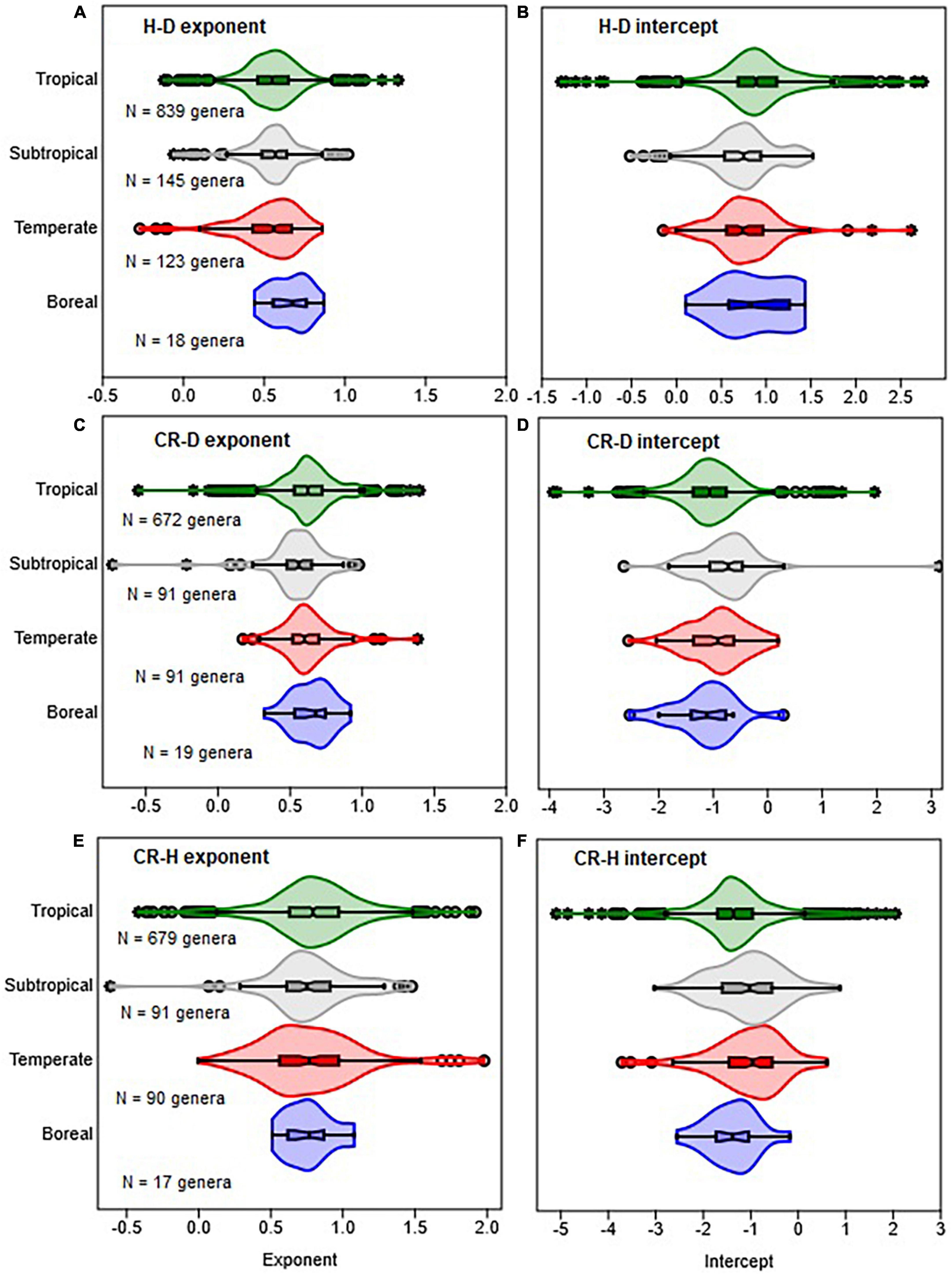
Figure 2. Comparison of climate zones in terms of the distribution of the allometric parameters of the scaling of height with stem diameter (H–D), crown radius with stem diameter (CR–D), and crown radius with stem height (CR–H). The distributions of exponents are shown in (A,C,E), while intercepts are in (B,D,F). The box and whisker plots display the median and its 95% CI (notches), lower quartile, upper quartile, extreme values, and outliers (O and *). Distributions in all cases are based on OLS estimates of the parameters for each genus.

TABLE 2

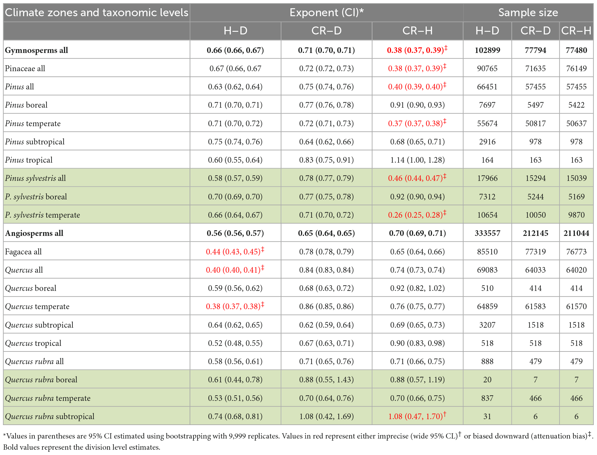
Table 2. Variations in the OLS estimates of the allometry exponents of stem height with diameter at breast height (H–D), crown radius with diameter at breast height (CR–D) and crown radius with stem height (CR–H) scaling with taxonomic levels and climate zones.

TABLE 3

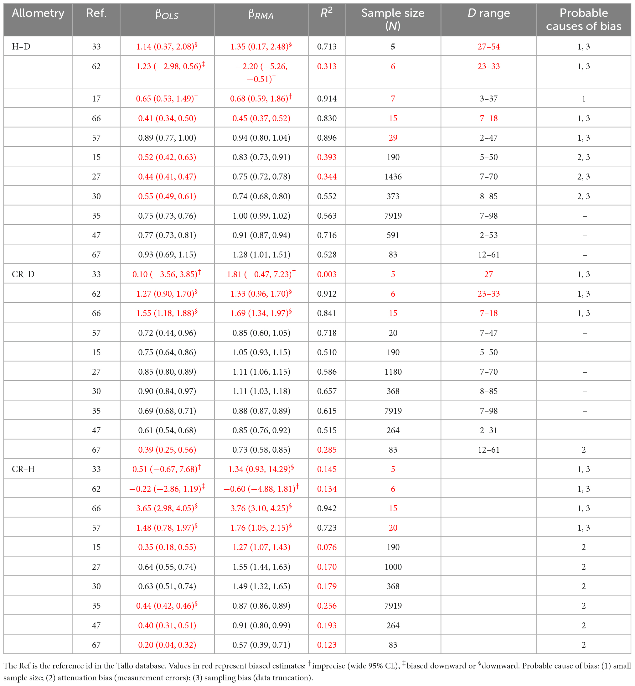
Table 3. Study-level variations in the OLS and RMA estimates (β_OLS and β_RMA) of the allometric scaling exponent of stem height with diameter at breast height (H–D), crown radius with diameter at breast height (CR–D) and crown radius with stem height (CR–H) of Pinus sylvestris in the temperate zone.

In the second set of analyses (Table 4), we compared H–D, CR–D, and CR–H allometric parameters of selected genera occurring in high and low disturbance areas in temperate climate. In a recent analysis, Sommerfeld et al. (2018) reported that high disturbance landscapes were dominated by the genera Picea, Abies, Pseudotsuga, and Pinus in the northern hemisphere. Low disturbance landscapes were largely dominated by broadleaved trees in the genera Nothofagus, Fagus, and Acer (Sommerfeld et al., 2018). Accordingly, we produced and compared the point estimates and the 95% CI of the allometry exponents of these species.

TABLE 4

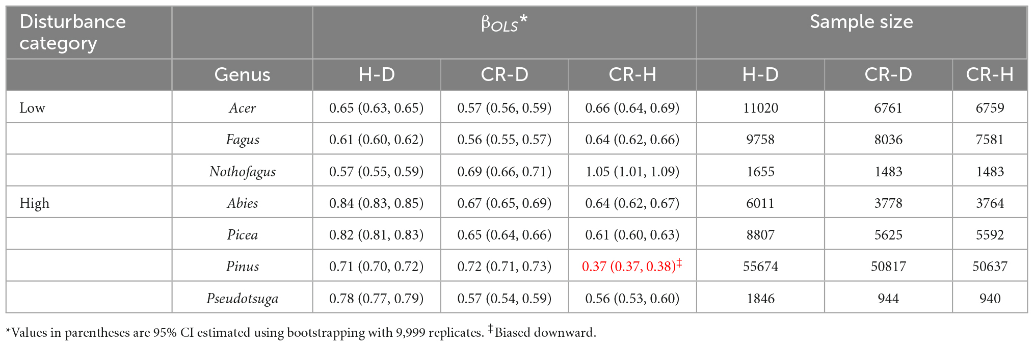
Table 4. Comparison of the phylogenetic allometry exponents (β_OLS) of the stem height to diameter (H–D), crown radius to diameter (CR–D), and crown radius to stem height (CR–H) scaling in genera in high and low disturbance temperate forest biomes.

In the third set of analyses, we compared the H–D, CR–D, and CR–H allometry exponents of the tallest and hyper-emergent trees species with medium and short-statured tree species in biomes with different historical disturbance regimes (Table 5 and Supplementary Table 2). We selected ten species from the list of the world’s tallest tree species available in Tng et al. (2012) including Sequoia sempervirens, P. menziesii, Sequoiadendron giganteum, and Picea sitchensis representing gymnosperms from North America; Eucalyptus regnans, Eucalyptus globulus, and Eucalyptus viminalis from Australia; Shorea faguetiana and Dinizia excelsa, which are the tallest tropical Angiosperm from rainforest in Asia and South America, respectively. Some of the species such as Eucalyptus regnans, P. menziesii, and S. giganteum are historically subjected to severe wildfires and are uniquely fire-resistant (Tng et al., 2012; Giunta et al., 2016). These giants are at the extreme tail of the tree height distribution and comparing them with medium to short-statured trees in other biomes is expected to provides an important case study for questions about allometric variation. Specifically, we selected Pinus ponderosa, a species adapted to low-moderate intensity fires in temperate North America (Giunta et al., 2016), and Colophospermum mopane, Combretum collinum, Combretum molle, Julbernardia paniculata, Vachellia seyal, and Vachellia tortilis from tropical savannas and woodlands in Africa. We also selected species from tropical rain forests in Africa (Piptadeniastrum africanum), Asia (Dryobalanops lanceolata, Parashorea tomentella, and Shorea fallax) and temperate and boreal forests (Abies sibirica, Acer platanoides, Fagus grandifolia, Fagus sylvatica, Nothofagus solandri, P. abies, Populus tremula, and P. tremuloides), which do not experience disturbances such as fire. We also included P. abies and P. tremuloides, which have a history of bark beetles and forest tent caterpillar outbreaks, respectively. When selecting the various species, we also made sure that sample sizes are adequate and the species broadly represent the biomes where they occur.

TABLE 5

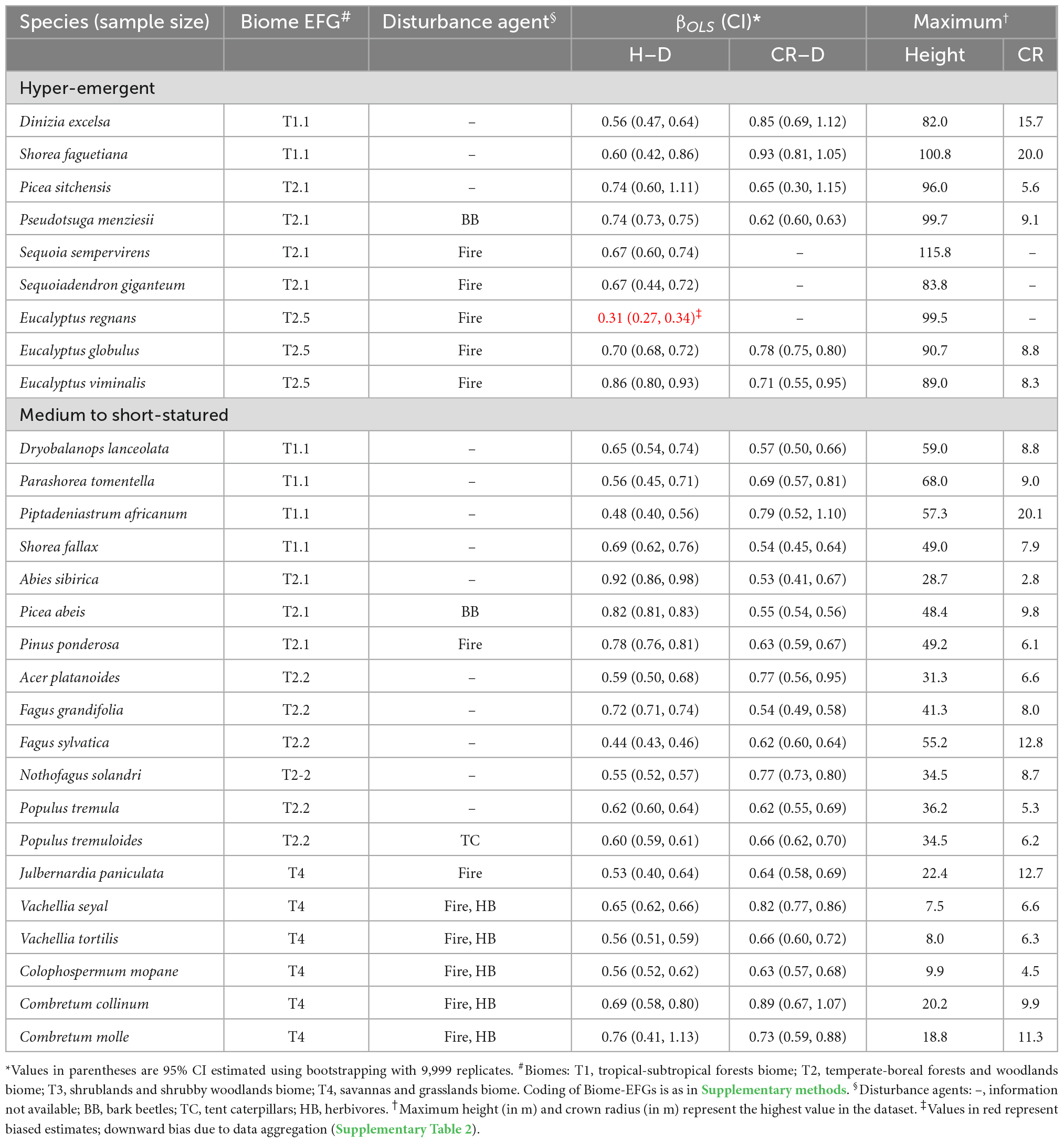
Table 5. Comparison of the allometry exponents (β_OLS) of the stem height to diameter at breast height (H–D) and crown radius to stem diameter (CR–D) scaling in nine of the world’s tallest and hyper-emergent tree species with medium to shorter tree species in different biomes.

In the fifth set of analyses, we compared allometric scaling of tree crown dimensions with stem diameter across tropical forests and savanna biomes in Africa, America, Asia, and Australia. For this analysis, we used data from the Forest Plots database² provided by Panzou et al. (2020). Here, we compared forests with savanna biomes across the tropics in terms of CD–D, Cdep–D, Cvol-D, and Cdep-CD allometry (Figures 3, 4 and Supplementary Table 3).

FIGURE 3

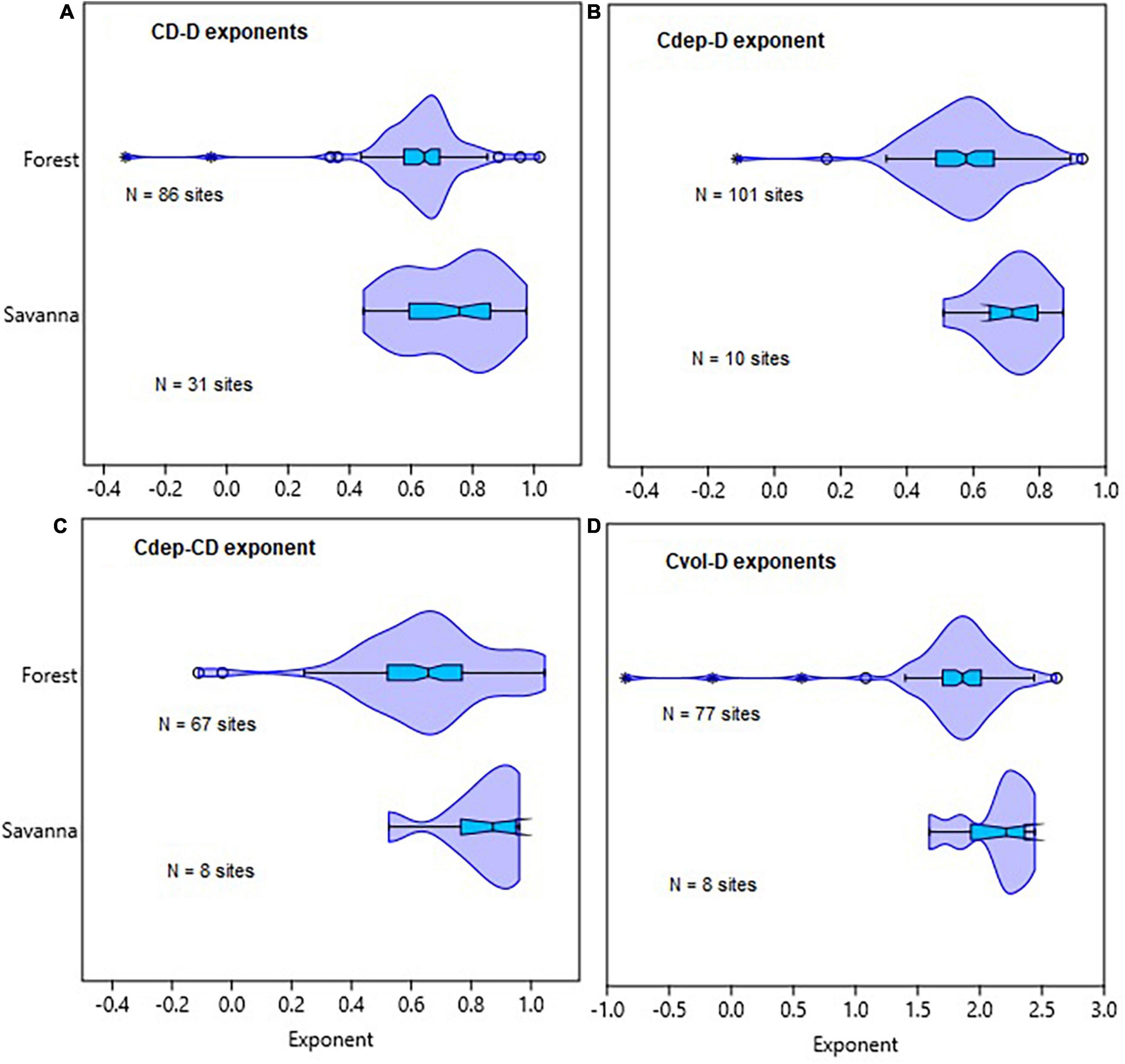
Figure 3. Comparison of tropical forest and savanna biomes in terms of the distribution of allometric exponents of crown diameter with stem diameter (CD–D), crown depth with stem diameter (Cdep–D), crown depth with crown diameter (Cdep–CD), and crown volume with stem diameter (Cvol–D) scaling. The distributions of exponents for the different allometric relationships are given in (A–D). The box and whisker plots display the median and its 95% CI (notches), lower quartile, upper quartile, extreme values and outliers (O and *).

FIGURE 4

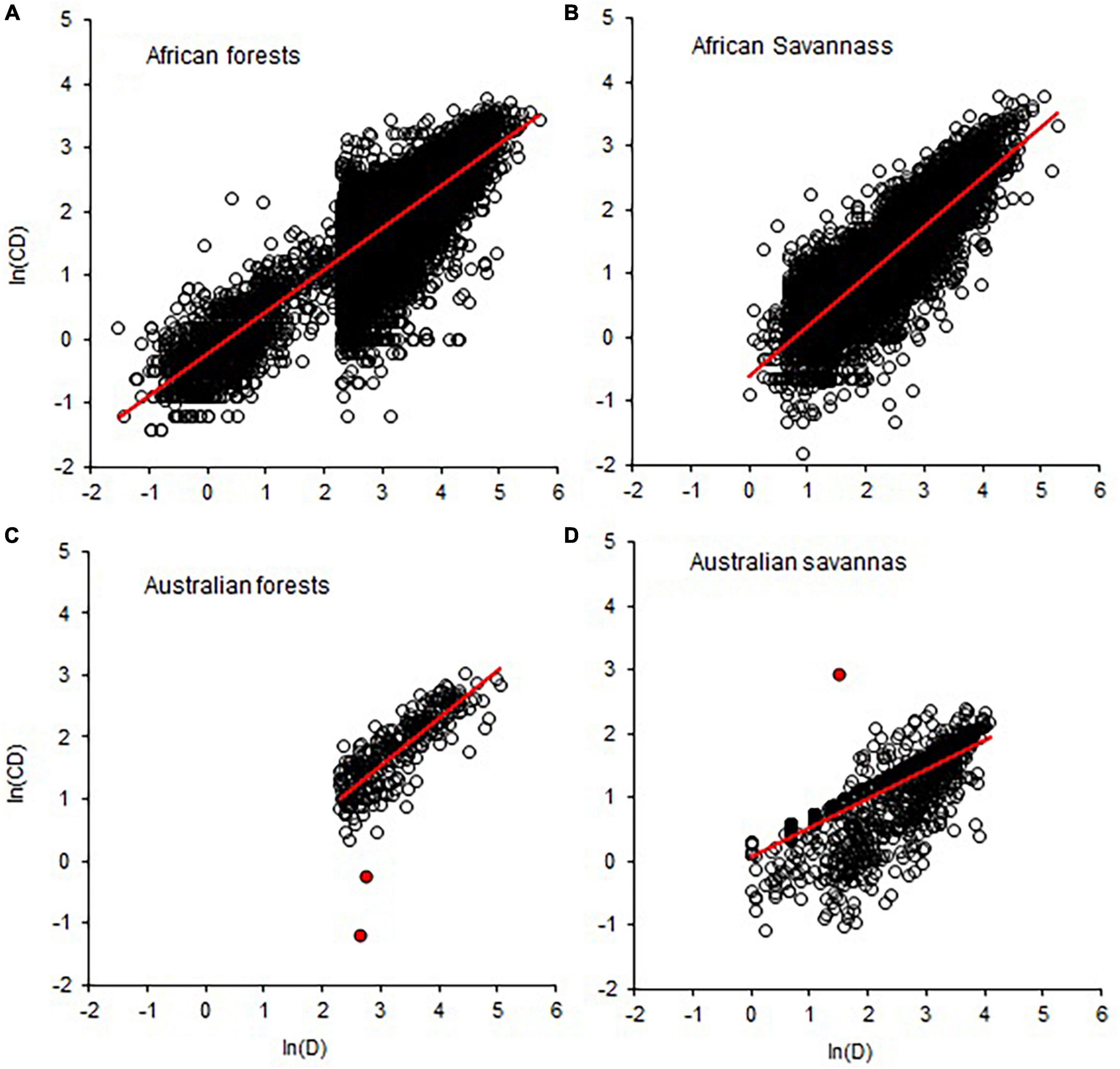
Figure 4. Comparison of forest and savanna biomes in terms of data quality in the allometric scaling of crown diameter with stem diameter (CD–D). Breaks in the distribution of values in A and B indicate the bias in sampling towards D > 5 (B) and D > 10 (A) and data truncation. Red circles in (C,D) are indicative of measurement errors. The red lines are OLS fitted lines.

Aboveground biomass vs. stem diameter or height

The allometric scaling of aboveground biomass with stem diameter (A–D) and aboveground biomass with stem height (A–H) is widely used to estimate aboveground carbon stocks as well as changes through time (Zianis and Mencuccini, 2004; Sileshi, 2014). The theoretical values of the A–D scaling exponent are 3, 5/2, and 8/3 according to the geometric similarity, stress similarity, and MST (Table 1). Similarly, the A–H exponents are 3, 5, and 4 according to the geometric similarity, stress similarity and MST, respectively (Table 1). The exponent is perceived as a distribution coefficient for the growth resources between A and D or A and H. For this analysis, we used raw data from Chave et al. (2014) to calculate allometry parameters per site for a mixed species of trees from a total of 58 sites across tropical Africa, Asia, and Americas. Then, we combined the values of the A–D allometric parameters with our own collection originally reported in Sileshi (2014). In total, there were 452 allometry exponents and their corresponding intercepts from various climate zones. For the A–H allometry we only had the 58 sites from Chave et al. (2014).

Belowground biomass vs. aboveground biomass

The partitioning of belowground plant biomass (B) with respect to aboveground biomass (A) is a key adaptive strategy of plants, which influences many functions in terrestrial communities. Allocation of belowground biomass relative to aboveground biomass has been traditionally analyzed using root (R) to shoot (S) ratio, which quantifies the relative proportion of growth resources allocated to roots versus shoots in a given condition. As measurement of belowground biomass is time consuming and expensive, allometric relationships have been proposed to estimate B from A (Cairns et al., 1997; Kuyah et al., 2016). At the level of individual plants, B has been shown to scale nearly isometrically (β = 1) with A across a broad-spectrum of vascular plants (Niklas, 2005; Cheng and Niklas, 2007).

To tests our hypotheses, we collected values of the B–A scaling exponent from the literature. We also analyzed datasets from our own studies and our colleagues. The first dataset consisted of biomass partitioning between shoot and root mass in seedlings of the fruit tree Uapaca kirkiana in the Miombo woodlands of Central Africa (Sileshi et al., 2007). The second and third dataset consisted of B–A scaling of miombo woodland trees in Zambia (Handavu et al., 2021) and Malawi (Kachamba et al., 2016). The fourth and fifth dataset consisted of the B–A scaling of Eucalyptus species in Kenya (Kuyah et al., 2013) and four tropical bamboos in India (Singnar et al., 2021), respectively. In all cases, we used the power function in the natural logarithm domain: ln(B) = ln(α)+β(lnA)+ε. When β = 1, B and A vary isometrically. When β < 1, shoots grow faster than roots, but allocation to roots is more than to shoots when β > 1 (Robinson and Peterkin, 2019).

Statistical analysis

Estimation of allometry parameters

Since allometry parameters can widely vary with regression techniques (Sileshi, 2014), initially we used non-linear regression (NLR), robust regression analysis (RRA), ordinary least square (OLS), reduced major axis (RMA), major axis (MA) regression, and linear mixed effects model (LMM). NLR, RRA, and OLS are called Model I regression while RMA and MA belong to the Model II regression (see Supplementary methods for details). We used the Paleontological Statistics (PAST) package³ to fit NLR, OLS, RMA, and MA, and the SAS system to fit LMM and RRA. We preferred the PAST package because it gives bootstrapped confidence intervals on the slope and intercept estimates (Supplementary methods). In the rest of this manuscript, we will focus on OLS and RMA estimates because they are more widely used in allometry (Hui et al., 2010; Kilmer and Rodríguez, 2017). RMA is also preferred where it is difficult to identify a variable as a dependent or independent variable (Hui et al., 2010. Past studies have focussed on comparing the empirical estimates of β with its theoretical value or among biomes using the t-test or the 95% CIs. Such comparisons are often fraught with errors due to low statistical power arising from small sample sizes. To avoid this problem, we analyzed the different datasets in two ways: (1) aggregated at different scales, namely, taxonomic divisions, climate zones and biomes; and (2) after disaggregating at the family and genus levels to compare climate zones and biomes in terms of the distribution of parameters. The first type of analysis involved regression of data aggregated at the level of taxonomic divisions (e.g., Gymnosperms vs. Angiosperms), climate zones (boreal, temperate, subtropical, and tropical) or biomes (e.g., forests and savannas) and comparing the point estimates and their 95% CI. When comparing categories, we applied the Johnson-Neyman technique (White, 2003) of first testing for homogeneity of residual variances (Vε), followed by null hypothesis (Ho) tests for equality of the slopes (Ho: β₁ = β₂) and intercepts (Ho: α₁ = α₂). We used Bartlett’s test of equality of variance when comparing the regression lines (Supplementary Table 5). We directly compared the exponents using the 95% CI only when P > 0.05. In all cases, we estimated the CIs using bootstrapping with 9,999 replications implemented in the PAST statistical package.

In the second type of analysis, we estimated the allometry parameters after disaggregating at the family, genus and species levels. Then, we compared taxonomic divisions and climate zones in terms of the empirical distributions of the exponents of H–D, CR–D, and CR–H scaling estimated at the family and genus levels. The same way, we compared the genera Pinus and Quercus after estimating the allometry parameters per species (Supplementary Figure 4). In the case of crown allometries (CD–D, Cdep–D, Cvol–D, and Cdep–CD), we estimated the exponents per study site as species names were unavailable. Then, we created violin plots of the exponents and intercepts to visualize their distributions among taxonomic divisions, climate zones (Figures 1–4) or genera (Supplementary Figure 4). In addition to the distributions, we complemented statistical inference with comparisons of the medians and their 95% CI (Supplementary Table 1). The 95% CI of medians are indicated by the notches in the box plots (Figures 1–3). The medians of two or more distributions are deemed not significantly different if their 95% CIs overlap (Krzywinski and Altman, 2014).

Assessing the effect of sample size and sampling bias on allometry parameters

In the analysis of P. sylvestris data (Table 3), we noted that the allometry parameters were biased wherever sample sizes (N) were <30 or when the samples consist of only small or large trees. Earlier work (e.g., Green, 1991) has also shown that unbiased estimates of regression parameters can be found only when N > 50+8P, where P is the number of parameters to be estimated. Therefore, we assessed the variations in allometry parameters with sample size in two separate analyses. In the first analysis, we categorized the estimated allometry parameters of H–D, CR–D, CR–H, and A–D based on the corresponding sample sizes into four classes: N < 10, 10–29, 30–60, and >60. Then, we created violin plots of the allometry parameters for each sample size class (Figures 3, 5 and Supplementary Figure 2) using the plot function of the PAST statistical package. In the second analysis, we explored the variations in the empirical estimates of exponents with sample size using locally weighted scatterplot smoothing (LOESS) implemented in the PAST statistical package (Figure 5D). PAST estimates the 95% confidence bands for the LOESS curves by bootstrapping using 9,999 random replications.

FIGURE 5

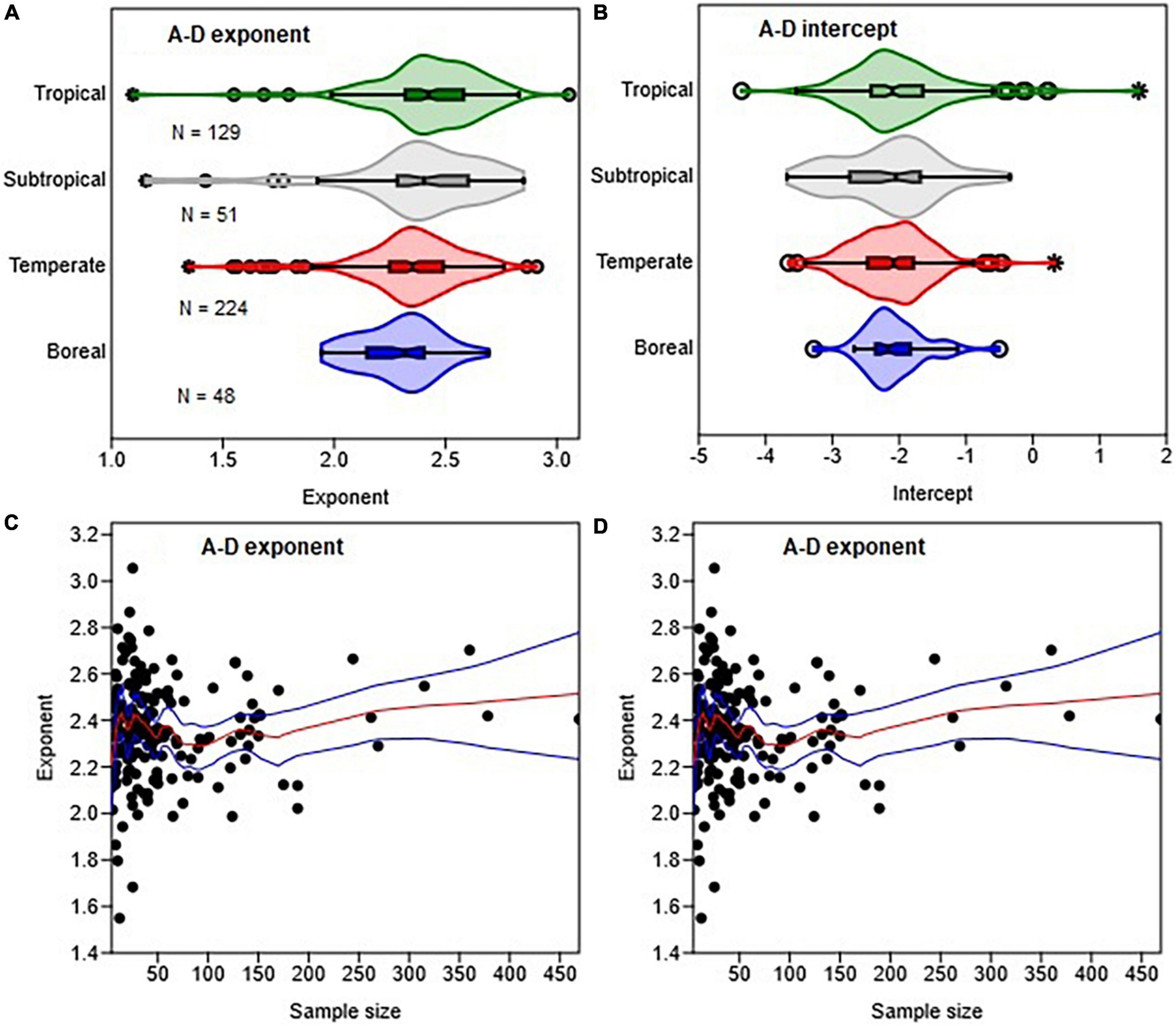
Figure 5. Variations in the distributions of the A-D allometric exponent (A) and intercept (B) with climate zones and sample size (C,D). The box and whisker plots display the median and its 95% CI (notches), lower quartile, upper quartile, extreme values, and outliers (O and *). The medians of two or more distributions are not significantly different if the 95% CIs overlap. In (D) the red and blue lines represent the LOESS trends and their 95% confidence bands.

Sampling bias is said to exist if the data are truncated (left or right) based on the diameter range in the database. Data truncation arises from sampling only those individuals whose size falls within a certain interval. Data are said to be left truncated when the lower segment of the population has been left out, for example, sampling predominantly large individuals as in Figure 4C. Right-truncation implies leaving out the upper segment of the population, for example excluding large sized individuals. We categorized the estimated allometry parameters of H–D and CR–D based on the minimum diameter (D) in the dataset into two classes: minimum D < 10 and >10 cm. Then, we created violin plots of the allometry parameters for minimum D class (Supplementary Figure 3). To reduce the confounding effect of sample size, we generated the plots for genera with N > 30.

Relationships between allometry parameters and divergence time

The objective of this analysis was to determine the relationships between (1) divergence time and the exponent at the family level, and (2) β and α in the various allometries. For analysis of the trends in allometric trajectories with evolutionary time, we obtained the divergence times (in million years ago = MYA) for Angiosperm families from Li et al. (2019) and Gymnosperm families from Lu et al. (2014). We explored the trends in the exponents and intercept with divergence time using LOESS implemented in the PAST statistical package (Figure 6). We could not do the same analysis for genera as we did not find the relevant divergence times of general.

FIGURE 6

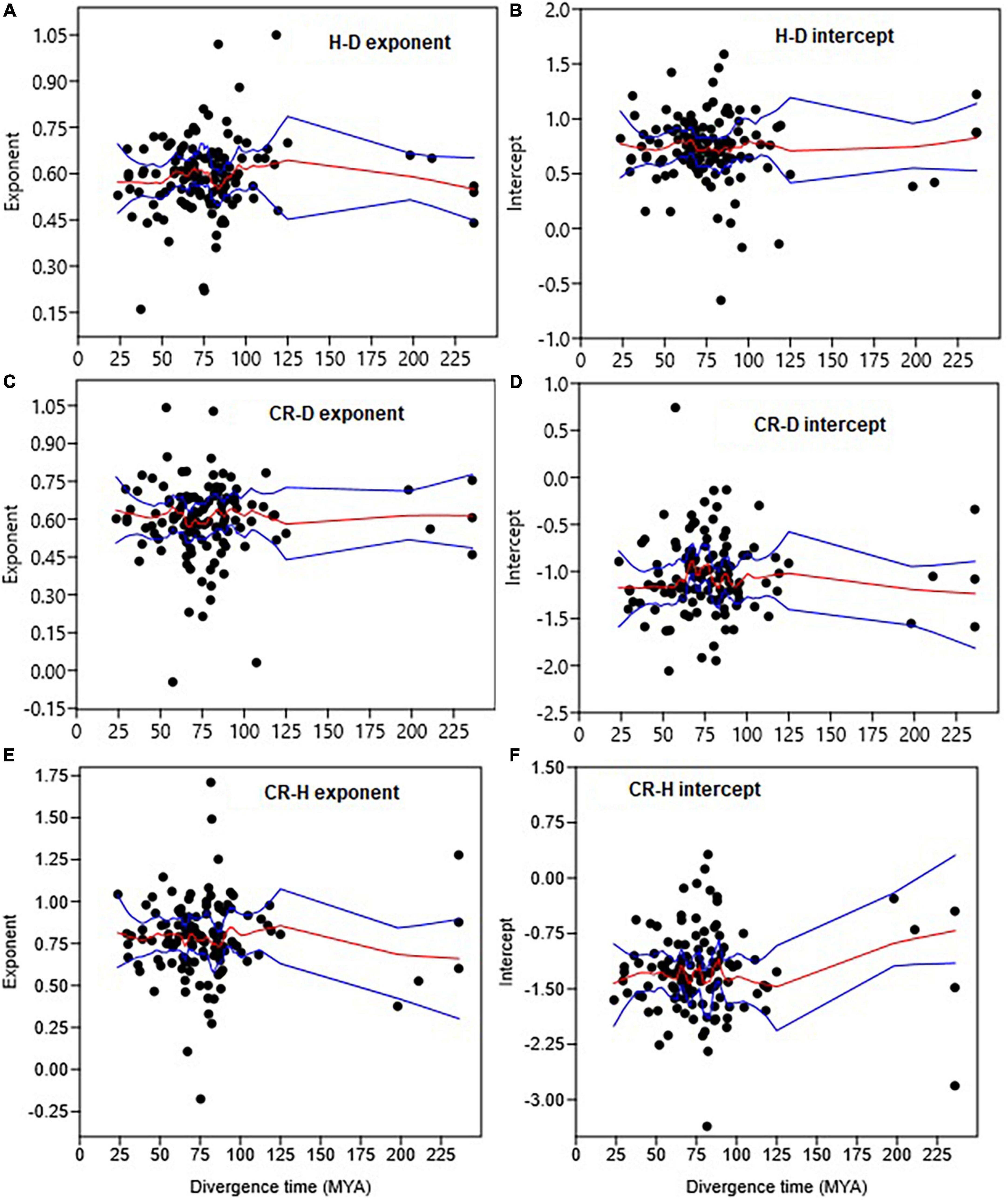
Figure 6. Trends in the H–D, CR–D, and CR–H allometry parameters with the median divergence time (in MYA = million years ago) of Gymnosperm and Angiosperm families. The trends in exponents are shown in (A,C,E), while trends in intercepts are in (B,D,F). The red and blue lines represent the LOESS smoothing curve and it 95% confidence limits, respectively.

Since the functional relationships between β and α were not clear, we created scatter plots of β on ln(α) for the allometric relationships analyzed at the different scales (Figure 7 and Supplementary Figure 5). Then, we tested whether or not a significant linear trend exists between β and ln(α).

FIGURE 7

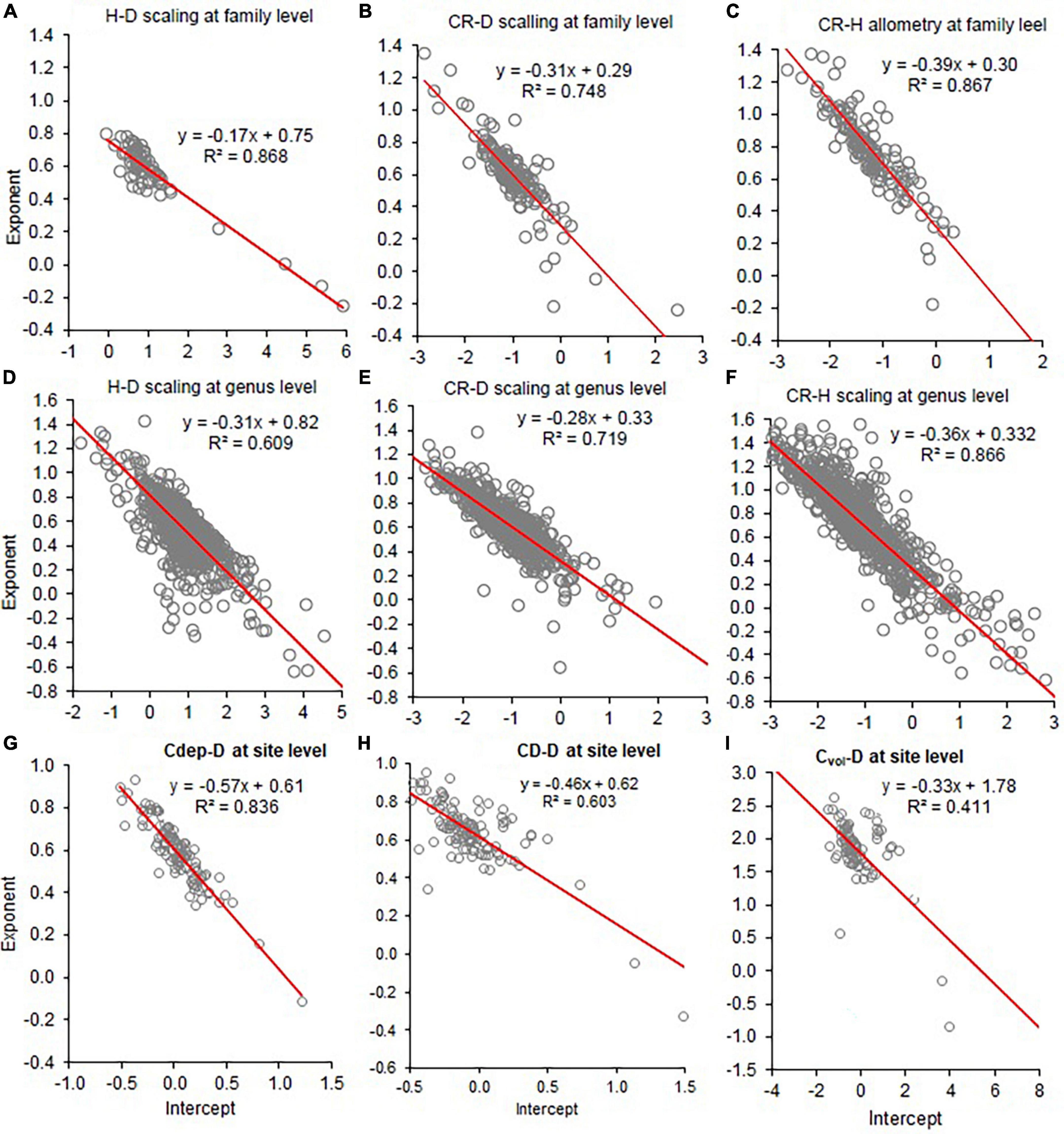
Figure 7. Co-variation of the allometry exponents (β) with the intercepts (Inα) of height to stem diameter (H–D), crown radius to stem diameter (CR–D), crown radius to stem height (CR–H), crown depth to stem diameter (CDep–D), crown diameter to stem diameter (CD–D), and crown volume to stem diameter (Cvol–D) at the family (A–C), genus level (D–F), and sites (G–I). The red line represents the fitted line of the linear regression of β on Inα.

Results

Stem diameter, height, and crown dimensions

The distributions of the H–D, CR–D, and CR–H allometry parameters revealed significant overlap between Gymnosperms and Angiosperms (Figure 1 and Supplementary Figure 1). When estimated at either the family or genus levels, the median values of the exponents of Gymnosperms and Angiosperms were also not significantly different from each other (Supplementary Table 1). Similarly, there was significant overlap between the distributions of exponents in the different climate zones (Figures 2A, B). The median values also did not significantly differ among climate zones (Supplementary Table 1). Except for the extreme values and outliers, the exponents predominantly fell within the range of theoretical values in Table 1. The distributions of exponents were more consistent with MST (β = 2/3) than the geometric (β = 1) or stress similarity (β = 1/2) hypothesis (Figures 1, 2). Values <1/2 or >1 were mostly artifacts of small sample size (N) estimation (Figure 8 and Supplementary Figure 2). All of the large outliers were associated with N < 10. When sample sizes exceeded 60, estimates of the allometry parameters [both β and ln(α)] fell in a narrower range than when N < 30 (Figures 8A, C, E and Supplementary Figure 2). The LOESS trend lines show that the exponents tended to stabilize around the MST exponent as sample sizes increased (Figures 8B, D, F). The minimum diameter in the sample also had significant effects on the H–D, CR–D, and CR–H exponents (Supplementary Figure 3). Across climatic zones, the H–D exponent was smaller when the minimum D was >5 cm compared to samples that include smaller trees D < 5 cm. The distributions of exponents of H–D,CR–D, and CR–H allometry calculated at the species level are shown here using Pinus and Quercus species as examples (Supplementary Figure 4). As in the family- and genus-level analysis above, the distributions of exponents were more consistent with MST than the geometric and stress similarity hypotheses.

FIGURE 8

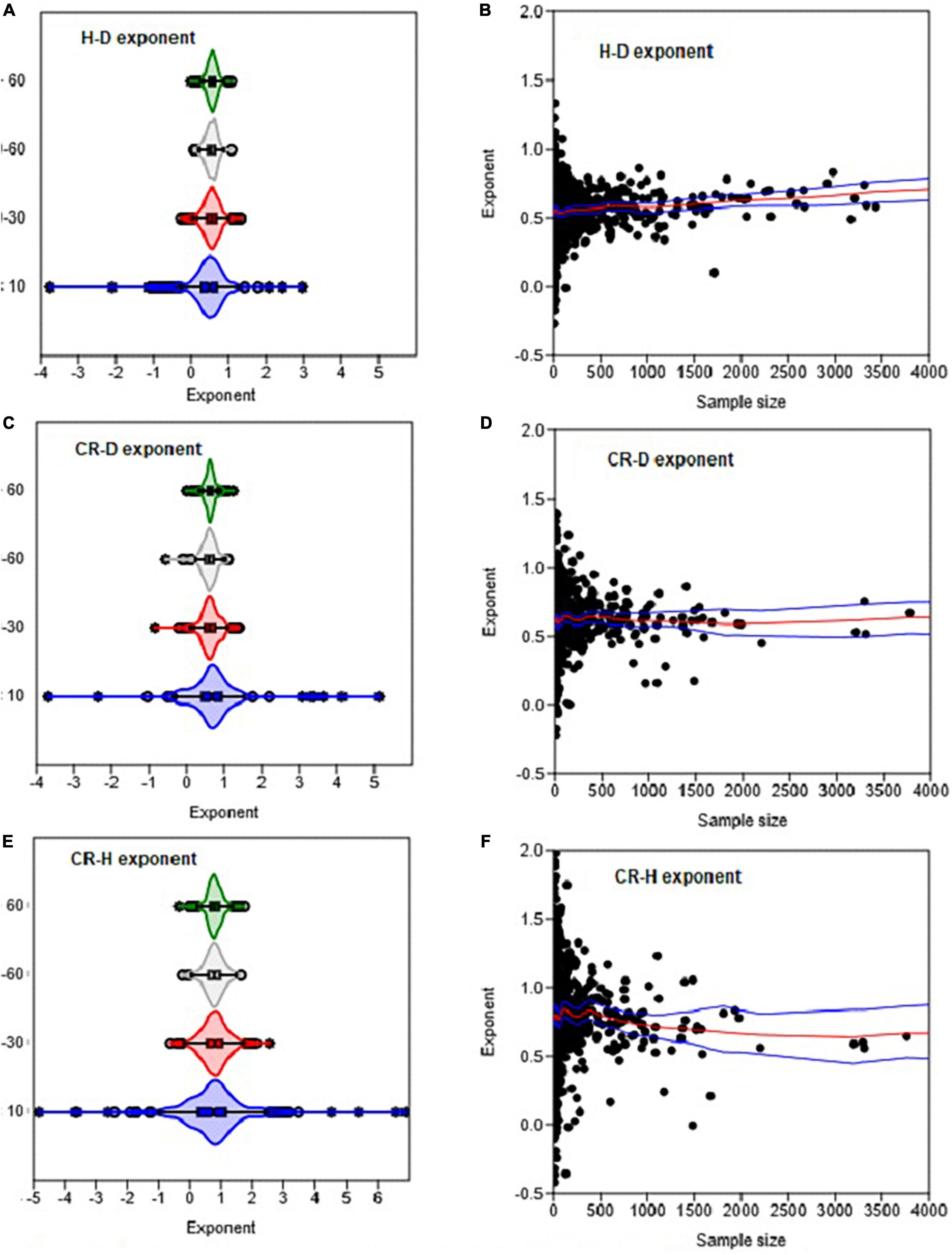
Figure 8. The effects of sample size on the variation in the H–D, CR–D, and CR–H allometric exponents (β). Distributions in (A,C,E) are based on OLS estimates of the exponent for each genus. Each circle in (B,D,F) represents the estimate of the exponent of a genus. The box and whisker plots display the median and its 95% CI (notches), lower quartile, upper quartile, extreme values, and outliers (O and *). In (B,D,F) the red and blue lines represent the LOESS trend lines and their 95% confidence bands.

When data were analyzed after aggregating at different scales, the OLS estimate of the exponent was significantly smaller for angiosperms (CI: 0.56, 0.57) than the theoretical value of 2/3 but larger than 1/2. The exponent of gymnosperms (CI: 0.65, 0.67) was consistent with MST (Table 2). On the other hand, the RMA estimates for both angiosperms (CI: 0.75, 0.77) and gymnosperms (CI: 0.88, 0.89) were significantly larger than 1/2 or 2/3 but smaller than 1. Further analysis of the H–D and CR–D allometry did not reveal systematic variations in the exponent with taxonomic levels (Table 2). In the majority of cases the exponents were closer to 2/3 than 1/2 or 1. Unlike in Angiosperms, the exponents of the CR–H allometry in Gymnosperms were mostly biased downward (Table 2). The CR–H exponent was precisely biased downward in P. sylvestris in temperate zones (Table 2). To see whether different model fitting techniques will change the outcome, we compared non-linear regression, OLS, RRA, RMA, MA, and LMM analysis of the CR–H scaling in P. sylvestris in temperate zones. The non-linear regression exponent of 0.25 (CL: 0.24, 0.27), OLS exponent of 0.26 (CI: 0.25, 0.28), RRA exponent of 0.32 (CI: 0.30, 0.34), and LMM exponent of 0.45 (CI: 0.43, 0.47) were significantly smaller than the MA exponent of 0.61 (CI: 0.58, 0.65) and RMA exponent of 0.85 (CI: 0.84, 0.87) for the same species. The discrepancies between Model I (OLS and RRA) and Model II (RMA and RMA) estimates are indicative of large errors in measurement of H.

In-depth analyses of H–D, CR–D, and CR–H allometry in P. sylvestris revealed how study-level estimates of the allometry exponents can be biased by a combination of small sample sizes, sampling bias and attenuation bias (Table 3). Attenuation bias is more evident in CR–H and H–D than in CR–D allometry indicated by the large discrepancies between OLS and RMA estimates of the exponent (Table 3).

Comparisons of the allometry exponents of the H–D, CR–D, and CR–H scaling in genera with high and low disturbance regimes are summarized in Table 4. All genera in the high disturbance regime had significantly higher H–D exponents than those in low disturbance regimes. On the other hand, the CR–D and CR–H scaling exponents did not show consistent differences between trees growing in high and low disturbance regimes (Table 4). Almost all of the exponent were significantly higher than the stress similarity exponent and lower than the geometric similarity exponent, but closer to the MST exponent.

Comparison of the exponents of hyper-emergent trees species with medium and short-statured species did not reveal systematic variations (trends) with tree size (Table 5). The H–D and CR–D exponents of hyper-emergent species were in the same range as those of the medium to short statured species (Table 5). For example, the H–D exponents of S. sempervirens and S. giganteum (0.67) are statistically indistinguishable from P. tremuloides (0.64), V. seyal (0.65), and C. collinum (0.69) although they occur in different climate zones, biomes and disturbance regimes (Table 5). Similarly, the CR–D exponent of P. menziesii (0.57) is statistically indistinguishable from Picea abies (0.57) and C. mopane (0.63) despite the differences in the climate zones, biomes and disturbance regimes (Table 5). The H–D and CR–D exponents of almost all species in Table 5 did not conform to the geometric similarity hypothesis (β = 1). With the exception of E. regnans, the majority of the exponents fell within the range of values assumed in stress similarity and MST. In-depth analysis at the site level data indicated that curious case of E. regnans arose due to aggregation of data of varying quality (Supplementary Table 2). The probable causes of the bias become clear when the data from each Reference ID were analyzed separately (see Supplementary Table 2 for details). These problems could not be remedied by application of more sophisticated analyses such as robust regression (Supplementary Table 2).

Comparisons of tropical forests with savanna biomes in terms of CD–D, Cdep–D, Cdep–CD, and Cvol–D also revealed broadly overlapping distributions of the exponents (Figure 3). The distributions of exponents were closer to the MST exponents than the geometric similarity and stress similarity exponents (Figure 3). Comparison of the point estimates (and CIs) of the exponents of CD–D also did not reveal systematic variations with biomes or continents (Supplementary Table 3). Where such differences exist, differences in sample size and sampling bias seem to play a role. For example, the sample size for American forests was 113 times larger than for American savannas. The diameter range reflects sampling bias toward larger trees in American forests than in the savannas. Therefore, the comparisons among the forest and savanna biomes are confounded by the differences in the diameter ranges and sample sizes. Asian forests and Australian savannas had exponents biased downward partly due to aggregation of data of varying quality. Graphic comparison of CD–D allometry in African and Australian forests and savannas reveals further insights into the degree of sampling bias (Figure 4). Sampling bias toward large trees is more evident in data from Australian forests (Figure 4C) and African savannas (Figure 4B). In four out of the seven African countries the minimum D was 10 cm, while in the remaining three countries the minimum D was 0.2–6.3 cm. These differences are reflected in the two groups of data in Figure 4A. Measurement errors are also evident in Figures 4C, D. Close examination also revealed that data from one site in Asia (Mala_8) was weighing down the exponent estimated for the whole continent (Supplementary Table 3). The Mala_8 site had two populations with non-overlapping distributions, one of which was of very poor data quality (Supplementary Table 3).

Statistical tests of differences in Cdep–D, Cvol–D, and Cdep–CD allometry between tropical forest and savanna biomes are summarized in Supplementary Table 5. With the exception of Cvol–D allometry, tropical forests and savannas did not significantly differ in their exponents. In the case of Cvol–D, the OLS estimate of the exponent was biased downward in tropical forests than in savannas, but the RMA estimates are comparable (Supplementary Table 5).

Aboveground biomass vs. stem diameter or height

The distributions of the A–D exponents in the different climate zones were significantly overlapping (Figure 5A). The median value of the exponents – 2.32 (CI: 2.25, 2.36) in boreal, 2.35 (CI: 2.34, 2.39) in temperate, 2.40 (CI: 2.34, 2.47) in subtropical and 2.42 (CI: 2.41, 2.48) in tropical zones – are statistically non-significant. The median values of the A–H exponents in the tropical biomes, where data were available, was 3.45 (CI: 3.18, 3.77). In all cases, the distributions of exponents were more consistent with the stress similarity and MST exponents than the geometric similarity exponent (Figure 5A). Tropical, subtropical and temperate regions had a large number of outliers of the A–D exponent. The total sample size available for analysis had significant effects on the A–D exponent (Figure 5C). There were large outliers when N < 30 than N > 60 trees (Figure 5C). The LOESS trend lines show that the exponent tended to approach the MST exponent as sample sizes increased (Figure 5C).

Belowground biomass vs. aboveground biomass

The 95% CI of the B–A exponents shows that in the majority of cases the exponent conforms with isometric scaling. The exponents also did not systematically vary with climate zones (Table 6). Except in a few cases, the RMA estimate of the B–A exponent in the different climate zones did not significantly differ from 1 (Table 6).

TABLE 6

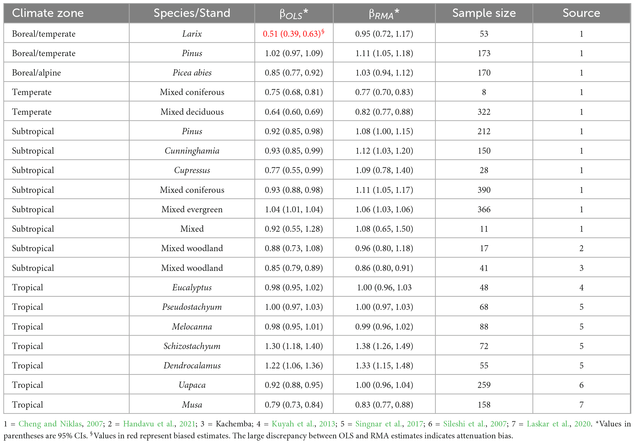
Table 6. Variations in the OLS and RMA estimates of the exponent (β_OLS and β_RMA) of the allometry of belowground biomass with aboveground biomass (B–A) in trees, bananas and bamboos across different climate zones and biomes.

Trends in allometry parameters

The analyses did not reveal significant trends in the allometry parameters of the H–D, CR–D, and CR–H scaling along the divergence times of Gymnosperm and Angiosperm families (Figure 6). Within Angiosperms the H–D allometry exponent of the more recent (∼29 MY old) family Bignoniaceae (β = 0.68) was not significantly different from those of the older (113–125 MY old) families Magnoliaceae (β = 0.68) and Winteraceae (β = 0.70). The H–D exponent of the more recent (∼24 MY old) Angiosperm family Staphyleaceae (β = 0.53) was also not significantly different from those of the older (∼236 MY old) Gymnosperm families Araucariaceae (β = 0.54), Podocarpaceae (β = 0.56), and Taxaceae (β = 0.44). The CR–D and CR–H allometries followed trends similar to H–D.

The analyses also revealed significant negative correlations between ln(α) and β in the allometries analyzed at the different scales (Figure 7 and Supplementary Figure 4). As a result, when ln(α) was biased upward, β was biased downward. We noted significant positive correlations between the CR-D and CR–H exponents (r = 0.647; P < 0.0001). Similarly, we observed a positively correlation (r = 0.543; P < 0.0001) between H–D and A–D exponents (Supplementary Figure 5) indicating tight co-variations among D, H, CR, and biomass.

Discussion

Stem diameter, height, and crown allometry

Our analyses have uncovered a tight co-variation among stem height, diameter, crown dimensions and tree biomass, consistent with allometric theory (e.g., Niklas and Spatz, 2004; West et al., 2009). The various analyses did not reveal evidence of systematic variations in the H–D, CR–D, and CR–H allometry with taxonomic level, evolutionary time, climate zones or biomes. These findings are consistent with the allometry constraint hypothesis, which posits that the evolutionary divergence of traits is restricted by integrated growth regulation, and thus β remains constant at macro-evolutionary timescales (Voje et al., 2013). The results are also in agreement with those of Blanchard et al. (2016), who found no significant variation in CA–D allometry across five biogeographic areas. According to Blanchard et al. (2016), the stability in CA–D allometry suggests that some universal constraints are sufficiently pervasive to restrict the variation of the exponent in a narrow range.

Unlike the H–D and CR–D scaling, the CR–H allometry was more variable probably because both H and CR are associated with greater measurement error than D (Ducey, 2012; Calders et al., 2015; Blanchard et al., 2016). Contrary to recent reports (e.g., Shenkin et al., 2020; Panzou et al., 2021), our analyses did not reveal significant differences in crown allometry between savanna and forest biomes. Our analysis also casts doubt over the notion that the H–D allometry depends on the context in which a tree grows and hence the exponent varies widely [references cited in Osunkoya et al. (2007), Watta and Kirschbaum (2011); Fortier et al. (2015), Hulshof et al. (2015), and Motallebi and Kangur (2016)]. Some of the past studies did not have adequate sample sizes and/or did not adequately control for differences in sample size and size-frequency distributions resulting in conflation of statistical artifacts with violations of allometric relationships. For example, Osunkoya et al. (2007), used small sample sizes (10–39 trees) and found wide variability in the exponent of the H–D scaling in 22 species. Watta and Kirschbaum (2011) reported that the exponents of the H–D relationship ranged between 0.73 and 1.43 across 84 plots, and this clearly violates the assumptions underlying allometric relationships. However, close examination of their report reveals differences in both the diameter range (D < 10 cm vs. D > 10 cm) and sample size between the two groups. Similarly, Fortier et al. (2015) reported differences in H–D exponents between moderate and high fertility sites. However, the diameter range of trees from the moderate fertility site (D = 10–27 cm) was smaller than the high fertility site (D = 20–38 cm) besides the very small sample sizes used (12) at each site. Even if sample sizes were large, the difference in the diameter range alone could have resulted in the observed differences in exponents. Here, we do not claim that the allometry exponent is static, but its variability is conflated with sampling bias and low statistical power due to small sample sizes. Unlike previous studies, our use of parameter distributions reveals the reality better than point estimates and their 95% CIs which are sensitive to differences in sample sizes and sampling bias. Our inferences are also based on disaggregated data and hence the agreement with allometry theory.

In previous studies, inferences have been solely based on point estimates and their 95% CI derived from aggregated data. For example, in Panzou et al. (2021) complex LMMs were implemented using aggregated data, which are prone to violations of LMM assumptions. We suspect this is the source of the counterintuitive values of the exponent reported in Panzou et al. (2021) for the American forests, American savannas, Asian forests, Australian forests and Australian savanna (Supplementary Table 3). The problem with aggregated data is that they are prone to contamination with poor quality data as is the case with E. regnans (Supplementary Table 2) and Asian forests (Supplementary Table 3). Data aggregation is known to leave analyses vulnerable to aggregation bias or ecological fallacy, i.e., drawing of false inferences about individual behavior on the basis of aggregate level statistics (Pollet et al., 2015; Salkeld and Antolin, 2020).

In a nutshell, the data does not support our hypothesis that the allometry exponents systematically vary with taxonomic levels, divergence time or climate zones. The data does not also support our hypothesis that trees adapted to different disturbance regimes have different allometry exponents. Although disturbance regimes are said to be critical in driving local to regional-scale variance in tree allometry relationships (Wenyan et al., 2022), the evidence seems to be weak. For example, Wenyan et al. (2022) found crown allometry exponents that conform to theoretical predictions in gap forest sites (created by cutting trees), and greater deviations from theoretical predictions in unmanaged forest sites. Indeed, their finding is contrary to the common notion that forests that have undergone disturbance deviate substantially from theoretical predictions.

Our initial hypothesis that hyper-emergent and short-statured tree species follow different allometric trajectories was also not supported. According to Osunkoya et al. (2007), H–D scaling in understory species follows a geometric similarity, while mid-canopy and emergent species follow stress–elasticity similarity. Close examination of their reports revealed that some of the heterogeneity in exponents is an artifacts of small sample sizes and inferences based on point estimates.

Aboveground biomass vs. stem diameter or height

Despite the wide variability in sample size and sampling conditions, the A–D exponents did not significantly vary with climate zones. They were also closer to the theoretical values of 5/2 and 8/3 for A–D allometry and 3–4 for A–H allometry. This is consistent with Zianis and Mencuccini (2004) who noted that there is a general convergence of the scaling exponents despite the multitude of factors affecting tree growth in different sites. Allometry theory (Enquist et al., 1999; Enquist and Niklas, 2002; Niklas and Enquist, 2002) and empirical results (e.g., Kuyah et al., 2013; Sun et al., 2022) also predict the same exponent for the allometric relationships between the different biomass components (i.e., stem, branch, foliage and root) and D. For example, in our re-analysis of data from Kuyah et al. (2013), the exponent was 2.50 for stem biomass to D allometry, 2.68 for branch biomass to D allometry, 1.87 for foliage biomass to D allometry and 2.45 for root biomass to D allometry. Similarly, in Sun et al. (2022) the exponent was 2.176 for stem biomass to D, 2.334 for branch biomass to D, 1.578 for foliage biomass to D and 2.063 for root biomass to D allometry although biomass allocation to stem, branch, foliage, and root biomass significantly differed. The exponent was also estimated at 2.196 for total woody biomass to D allometry, 2.235 for aboveground woody biomass to D allometry (Sun et al., 2022). The closeness of these figures indicate that the different biomass components follow the same scaling rules and allocation patterns.

Our earlier review (Sileshi, 2014) and the present analysis reveal that the exponents reported in the literature are biased downward partly due to the small sample sizes used in individual studies. Duncanson et al. (2015) showed that the use of small sample sizes in allometric equations can result in positive bias of ∼70% in the average site-level biomass estimates. In the past, the limiting factor has been the time and resources needed for destructive sampling of a large number of trees (Duncanson et al., 2015). With the increasing availability of portable ground-based LiDAR (Calders et al., 2015), data for large sample sizes can be acquired quickly, including samples of very large trees for which destructive sampling would be logistically impractical (Duncanson et al., 2015).

The power function has been reported to perform equally or even outperform other models in many situations (e.g., Sileshi, 2014; Sun et al., 2022; Wenyan et al., 2022). However, the debates over perceived variability of β has been discouraging practitioners from using simple power law models. As a result, empirical models of statistically dubious quality continue to proliferate the biomass estimation literature (Sileshi, 2014). Here we have shown that the variability in β is mostly an artifact of small sample sizes and sampling bias toward large trees. In forest inventories, it is a common practice to measure trees above a certain stem diameter, e.g., D > 5 cm or even >10 cm. Biomass estimation models developed using trees with D > 10 cm tended to overestimate the mean diameter ($\overline{X}$) and ln(α) resulting in underestimation of β (see Equation 4 below). Therefore, we strongly recommend destructive sampling of trees including smaller stem diameter (e.g., 2.5 cm) during the development of biomass estimation models. We also recommend sampling roughly equal number trees from each diameter classes to get a truly representative sample of the size-frequency distribution of the target population [see Kuyah et al. (2013)]. When these statistical problems are remedied, the power law model could provide a more convenient tool for predicting forest biomass and carbon stocks at different scales. A model based on a tested and established theory is more likely to be robust to new information than those purely based on observed patterns and correlations, which may prove unstable when new information emerges.

Belowground biomass vs. aboveground biomass

Our analysis indicates that belowground biomass scales with aboveground biomass isometrically (β = 1) regardless of the context. This is consistent with allometric theory (Cheng and Niklas, 2007). This makes allometric models a more powerful tool than the traditional use of root-to-shoot ratios to predict belowground biomass. Root to shoot ratios often vary across biomes, vegetation types, taxonomic groups (Qi et al., 2019), growth stages and tree sizes (Peichl and Arain, 2007; Kuyah et al., 2013; Mašková and Herben, 2018). For example, a global analysis by Qi et al. (2019) found significantly higher root-to-shoot ratios in angiosperms than in gymnosperms. Similarly, Peichl and Arain (2007) and Mašková and Herben (2018) found decrease in root to shoot ratios with time and substrate nutrients. In contrast, a single allometric equation could predict total belowground biomass from aboveground biomass across the entire age-sequence (Peichl and Arain, 2007; Robinson and Peterkin, 2019).

Since there were not many datasets on changes in tree biomass allocation with taxonomic levels, disturbance regimes or stages of forest stand development, we were unable to investigate the B–A allometry in more detail. Biomass allocation also remains poorly documented in geoxyles, whose biomass is disproportionately found belowground. Geoxyles are plants with short-lived reproductive aerial branches and woody underground structures (xylopodia) (Maurin et al., 2014; Meller et al., 2022), and these are common in regions with frequent fires such as African savannas and the cerrado in Brazil (Maurin et al., 2014; Meller et al., 2022). Geoxyles may provide the next frontier of research in biomass allocation in biomes that experience frequent disturbance by fire.

Sources of bias and spurious exponents

In the literature, counterintuitive values of β have been reported and in some cases such values have been used to challenge predictions of allometry theories. For example, the MST has been challenged by a number of forest ecologist [see Shenkin et al. (2020) for details] for not providing coherent explanations for the variability in β. In the following sections we show how (1) spurious values of β can arise as statistical artifacts; (2) β varies with ln(α), and (3) the accuracy with which β is estimated depends on the sample size (N), measurement errors, the representativeness of the sample available for analysis and the regression technique used.

The various analyses in this study and earlier studies (e.g., Zianis and Mencuccini, 2004; Ducey, 2012; Sileshi, 2014; Zhang et al., 2016) have demonstrated an inverse linear relationship between the exponent and the intercept. This points to some kind of trade-off between ln(α) and β. One possible explanation is the principle of optimality in biological design (Popescu, 1998). Since natural selection leads to an economy of design, the parameter trade-off may be regarded as a manifestation of an attempt to achieve optimality. The observed co-variation between ln(α) and β is consistent with the power-law relationship in the logarithmic domain:

$\text{ln}(\alpha )=\overline{Y}-\overline{X}\beta (3)$

where $\overline{X}$ is the mean of log(X) and $\overline{Y}$ is the mean of log(Y). From equation 3 it follows that

$\beta =\frac{\overline{Y}-\ln (\alpha )}{\overline{X}}(4)$

This relationship implies that bias in ln(α) can result in biased estimates of β. For example, data in Figures 2, 3, 5 revealed that β values that are biased in one direction are associated with ln (α) values biased in the opposite direction. From Equation 4 it follows that an upward bias in ln(α) or $\overline{X}$ will result in a downward bias in β and vice versa. Biases in $\overline{X}$ typically arise from small sample sizes, sampling biases and measurement errors. For example, sampling bias toward large trees will result in an upward bias in $\overline{X}$ and ln(α), therefore a commensurate downward bias in in β.

From Figures 5, 8 it is evident that β estimates tend to be biased either downward or upward when sample sizes are small. Our findings reinforce earlier reports that allometry parameters are highly sensitive to sample size (Duncanson et al., 2015). When N < 30, the 95% CI also tend to be very wide, and cover different theoretical values of β (see Table 3). This makes it difficult to distinguish between the different theoretical predictions. Our review of the published exponents indicates that site-specific biomass models were particularly based on small sample sizes. For example, over 75% of the A–D scaling exponents in the literature were estimated using N < 60, of which 43% were based on N < 30 trees. Therefore, it is not surprising that the median value of the A–D exponents were smaller than the theoretical value of 8/3 (Figure 5). To achieve sufficient statistical power, we recommend the use of a minimum of 66 sample trees when estimating parameters of the power law model following the rule of thumb N > 50+8P proposed by Green (1991).

The accuracy with which β is estimated in OLS regression depends on the accuracy with which the X and Y variables were measured. Measurement errors cause a pervasive problem known as attenuation bias or regression dilution (Maroco, 2007; Hutcheon et al., 2010). OLS regression assumes that the X-variable is measured without error. In reality, tree dimensions such as D and H are measured with a great deal of error (see Supplementary methods). In the presence of measurement errors in X, estimators of the correlation coefficient (r) do not converge to their true population values (ρ) even if the sample size is infinitely large. Accordingly, β will be biased downward because it is a function of the correlation coefficient (r) between log(X) and log(Y), their variances (V_Y and V_X) and the covariance (i.e., COV_X,Y):

$\beta =r\sqrt{\frac{V_Y}{VX}}=r\frac{{\sigma }_Y}{{\sigma }_X}=\frac{CO{V}_{X,Y}}{V_X}(5)$

where σ_D and σ_Y are the standard deviation of log(X) and log(Y), respectively. Loken and Gelman (2017) showed that with large N, adding measurement error will almost always reduce the observed correlation (r) between X and Y. As such, β becomes more precisely biased toward zero as sample sizes increase (Maroco, 2007). From equation 5 it also follows that the sign of β depends entirely on the sign of r or COV_X,Y since σ_X, σ_Y and V_X are always positive. If the measurement errors in X are very large, the sign of r tends to be negative. This is probably why counterintuitive values of the exponent reported in the literature emerge.

The accuracy with which of β is estimated also depends on the representativeness of the sample of the underlying population. P. sylvestris (Table 3), Australian savannas (Figure 4) and E. regnans (see Supplementary Table 2) provide vivid examples of how sampling bias result in biased estimates of allometry parameters.

The various analyses (Tables 3, 6 and Supplementary Table 3) show that different regression techniques can lead to entirely different conclusions about the size of β for the same dataset. These differences arise due to the differences in the way in which measurement errors and outliers are handled within the different regression techniques (see Supplementary methods). At the different scales of analysis, we have shown that the RMA estimates of β are consistently larger than the OLS estimates, while LMM estimates are usually smaller than OLS estimates (Tables 3, 6 and Supplementary Tables 2, 3, 5). Elsewhere RMA was also reported to overestimate the true regression slope (Kilmer and Rodríguez, 2017). This is due to the mathematical relationship between the OLS and the RMA estimators of β. For r ≠ 0, β_RMA is the ratio between the β_OLS and r:

${\beta }_{RMA}=\frac{\left|{\beta }_{OLS}\right|}{r}=\frac{S{D}_Y}{S{D}_X}=\sqrt{\frac{V_Y}{V_X}}(6)$

β_RMA is also the ratio of SD_Y to SD_X (Sokal and Rohlf, 1995):

This implies that β_RMA will be biased upward if r is biased toward 0. Therefore, RMA can give a false impression of isometry when in reality the actual relationship is allometric.

Although LMMs provide a convenient framework to account for factors associated with site quality, climate, or stand history, in our analyses it yielded β estimators that were biased downward (Supplementary Table 5). We have also noted this problem in earlier studies (e.g., Panzou et al., 2021). It must be noted that LMMs are sensitive to violations of various assumptions (Schielzeth et al., 2020) and imbalances in sample size between categories. Allometry parameters in LMM can be biased due to these violations, and therefore empirical estimates should not be taken at face value.

Conclusion and recommendations

This study is the first of its kind in applying rigorous statistical tests on multiple allometries and visualizing the empirical distributions of parameters at different scales. The results show a striking similarity in allometry across taxonomic lineages, climate zones, biomes and disturbance regimes. Our main conclusions are: (1) the central tendency of the exponents is toward 2/3 for H–D, CR–D, CR–H, Cdep-D, and Cdep-CD allometry, 5/2–8/3 for A–D allometry, and 1 for B–A allometry across the different scales; (2) the exponent of these allometries has remained relatively constant through evolutionary time; (3) the exponent and the intercept are inversely related; and (4) some of the discrepancy between empirical estimates of the exponent and its theoretical value arises from statistical artifacts. These findings have both theoretical and practical implications. From a theoretical perspective, the findings provide novel insights into the puzzling variability reported in the exponents, which has been the sources of debates over the universality of allometric scaling and the validity of macro-ecological theories. In some of the literature we reviewed, authors seem to have conflated statistical artifacts with violations of allometric relationships.

The practical implication is that the simple power law model could provide a more convenient tool for predicting forest biomass and carbon stocks at different scales because it is grounded in sound theory and supported by empirical results. There are not many long-term studies that predict productivity across plant communities over time or at various successional stages and locations. Therefore, the use of allometric models can provide a viable alternative for predicting productivity. The other practical implication of our findings is that the exponent can either be underestimated or overestimated when the sample sizes are small, measurements errors are large, sampling is biased, data are aggregated and the wrong regression technique is used. Therefore, we strongly recommend practitioners of allometry to pay particular attention to statistical artifacts, and interpret results cautiously when comparing empirical values with theoretical predictions. We also strongly recommend the use of larger sample sizes and samples that are representative of the size-frequency distribution of the target population when testing hypothesis about allometric variation with climatic zones, biomes or disturbance regimes.

Data availability statement

The original contributions presented in this study are included in the article/Supplementary material, further inquiries can be directed to the corresponding author.

Author contributions

All authors listed have made a substantial, direct, and intellectual contribution to the work, and approved it for publication.

Acknowledgments

We are indebted to the researchers who made their data available in stand-alone databases, as supplementary online materials or within their publications, which have enabled us to re-examine earlier findings from a different perspective.

Conflict of interest

The authors declare that the research was conducted in the absence of any commercial or financial relationships that could be construed as a potential conflict of interest.

Publisher’s note

All claims expressed in this article are solely those of the authors and do not necessarily represent those of their affiliated organizations, or those of the publisher, the editors and the reviewers. Any product that may be evaluated in this article, or claim that may be made by its manufacturer, is not guaranteed or endorsed by the publisher.

Supplementary material

The Supplementary Material for this article can be found online at: https://www.frontiersin.org/articles/10.3389/ffgc.2022.1084480/full#supplementary-material

Footnotes

1. ^ https://doi.org/10.5281/zenodo.6637599
2. ^ https://doi.org/10.5521/forestplots.net/2020_8
3. ^ https://past.en.lo4d.com/windows

References

Blanchard, E., Birnbaum, P., Ibanez, T., Boutreux, T., Antin, C., Ploton, P., et al. (2016). Contrasted allometries between stem diameter, crown area, and tree height in five tropical biogeographic areas. Trees 30, 1953–1968. doi: 10.1007/s00468-016-1424-3

CrossRef Full Text | Google Scholar

Brown, J. H., Gupta, V. K., Li, B. L., Milne, B. T., Restrepo, C., and West, G. B. (2002). The fractal nature of nature: Power laws, ecological complexity and biodiversity. Philos. Trans. R. Soc. Lond. B 357, 619–626.

Google Scholar

Burton, P., Jentsch, A., and Walker, L. R. (2020). The ecology of disturbance interactions. BioScience 70, 854–870. doi: 10.1093/biosci/biaa088

CrossRef Full Text | Google Scholar

Cairns, M., Brown, S., Helmer, E., and Baumgardner, G. A. (1997). Root biomass allocation in the world’s upland forests. Oecologia 111, 1–11. doi: 10.1007/s004420050201

PubMed Abstract | CrossRef Full Text | Google Scholar

Calders, K., Newnham, G., Burt, A., Murphy, S., Raumonen, P., Herold, M., et al. (2015). Nondestructive estimates of above-ground biomass using terrestrial laser scanning. Methods Ecol. Evol. 6, 198–208. doi: 10.1111/2041-210X.12301

CrossRef Full Text | Google Scholar

Chave, J., Réjou-Méchain, M. E., Búrquez, A., Chidumayo, E., Colgan, M. S., Delitti, W. B. C., et al. (2014). Improved allometric models to estimate the aboveground biomass of tropical trees. Glob. Change Biol. 20, 3177–3190.

Google Scholar

Cheng, D. L., and Niklas, K. J. (2007). Above- and below-ground biomass relationships across 1534 forested communities. Ann. Bot. 99, 95–102. doi: 10.1093/aob/mcl206

PubMed Abstract | CrossRef Full Text | Google Scholar

Ducey, M. J. (2012). Evergreenness and wood density predict height–diameter scaling in trees of the northeastern United States. For. Ecol. Manage. 279, 21–26. doi: 10.1016/j.foreco.2012.04.034

CrossRef Full Text | Google Scholar

Duncanson, L., Rourke, O., and Dubayah, R. (2015). Small sample sizes yield biased allometric equations in temperate forests. Sci Rep. 5:17153. doi: 10.1038/srep17153

PubMed Abstract | CrossRef Full Text | Google Scholar

Enquist, B. J., and Niklas, K. J. (2001). Invariant scaling relations across tree dominated communities. Nature 410, 655–660. doi: 10.1038/35070500

PubMed Abstract | CrossRef Full Text | Google Scholar

Enquist, B., and Niklas, K. J. (2002). Global allocation rules for patterns of biomass partitioning in seed plants. Science 295, 1517–1520.

Google Scholar

Enquist, B. J., Economo, E. P., Huxman, T. E., Allen, A. P., Ignace, D. D., and Gillooly, J. F. (2003). Scaling metabolism from organisms to ecosystems. Nature 423, 639–642.

Google Scholar

Enquist, B. J., West, G. B., Charnov, E. C., and Brown, J. H. (1999). Allometric scaling of production and life-history variation in vascular plants. Nature 401, 907–911.

Google Scholar

FAO (2012). Global ecological zones for FAO forest reporting: 2010 update. Forest resources assessment working paper 179. Rome: Food and Agriculture Organization of the United Nations.

Google Scholar

Fischer, A., Marshall, P., and Camp, A. (2013). Disturbances in deciduous temperate forest ecosystems of the northern hemisphere: Their effects on both recent and future forest development. Biodivers. Conserv. 22, 1863–1893. doi: 10.1007/s10531-013-0525-1

CrossRef Full Text | Google Scholar

Fortier, J., Truax, B., Gagnon, D., and Lambert, F. (2015). Plastic allometry in coarse root biomass of mature hybrid poplar plantations. Bioenerg. Res. 8, 1691–1704. doi: 10.1007/s12155-015-9621-2

CrossRef Full Text | Google Scholar

Giunta, A. D., Jenkins, M., Hebertson, E. G., and Munson, A. S. (2016). Disturbance agents and their associated effects on the health of interior Douglas-fir forests in the central rocky mountains. Forests 7:80. doi: 10.3390/f7040080

CrossRef Full Text | Google Scholar

Green, S. B. (1991). How many subjects does it take to do a regression analysis? Multivar. Behav. Res. 26, 499–510. doi: 10.1207/s15327906mbr2603_7

PubMed Abstract | CrossRef Full Text | Google Scholar

Handavu, F., Syampungani, S., Sileshi, G. W., and Chirwa, P. W. C. (2021). Above-ground and below-ground tree biomass and carbon stocks in the miombo woodlands of the Copperbelt in Zambia. Carbon Manage. 12, 307–321. doi: 10.1080/17583004.2021.1926330

CrossRef Full Text | Google Scholar

Hlásny, T., König, L., Krokene, P., Lindner, M., Montagné-Huck, C., Müller, J., et al. (2021). Bark beetle outbreaks in Europe: State of knowledge and ways forward for management. Curr. For. Rep. 7, 138–165. doi: 10.1007/s40725-021-00142-x

CrossRef Full Text | Google Scholar

Hui, C., Terblanche, J. S., Chown, S. L., and McGeoch, M. A. (2010). Parameter landscapes unveil the bias in allometric prediction. Methods Ecol. Evol. 1, 69–74.

Google Scholar

Hulshof, C. M., Swenson, N. G., and Weiser, M. D. (2015). Tree height–diameter allometry across the United States. Ecol. Evol. 5, 1193–1204. doi: 10.1002/ece3.1328

PubMed Abstract | CrossRef Full Text | Google Scholar

Hutcheon, J. A., Chiolero, A., and Hanley, J. A. (2010). Random measurement error and regression dilution bias. BMJ 340:c2289.

Google Scholar

Huxley, J. S., and Teissier, G. (1936). Terminology of relative growth. Nature 137, 780–781.

Google Scholar

Jackson, T. D., Shenkin, A. F., Majalap, N., Jami, B., Sailim, A. B., Reynolds, G., et al. (2021). The mechanical stability of the world’s tallest broadleaf trees. Biotropica 53, 110–120. doi: 10.1111/btp.12850

CrossRef Full Text | Google Scholar

Jucker, T., Fischer, F. J., Chave, J., Coomes, D. A., Caspersen, J., Ali, A., et al. (2022). Tallo: A global tree allometry and crown architecture database. Glob. Change Biol. 28, 5254–5268. doi: 10.1111/gcb.16302

PubMed Abstract | CrossRef Full Text | Google Scholar

Kachamba, D., Eid, T., and Gobakken, T. (2016). Above- and belowground biomass models for trees in the miombo woodlands of Malawi. Forests 7:38. doi: 10.3390/f7020038

CrossRef Full Text | Google Scholar

Keith, D. A., Ferrer-Paris, J. R., Nicholson, E., Bishop, M., Polidoro, B. A., and Ramirez-Llodra, E. (2022). A function-based typology for Earth’s ecosystems. Nature 610, 513–518. doi: 10.1038/s41586-022-05318-4

PubMed Abstract | CrossRef Full Text | Google Scholar

Kelly, K. (2007). Sample size planning for the coefficient of variation from the accuracy in parameter estimation approach. Behav. Res. Methods 39, 755–766. doi: 10.3758/bf03192966

PubMed Abstract | CrossRef Full Text | Google Scholar

Kerkhoff, A. J., and Enquist, B. J. (2006). Ecosystem allometry: The scaling of nutrient stocks and primary productivity across plant communities. Ecol. Lett. 9, 419–427. doi: 10.1111/j.1461-0248.2006.00888.x

PubMed Abstract | CrossRef Full Text | Google Scholar

Kerkhoff, A. J., Enquist, B. J., Elser, J. J., and Fagan, W. F. (2005). Plant allometry, stoichiometry and the temperature-dependence of primary productivity. Glob. Ecol. Biogeog. 14, 585–598.

Google Scholar

Krzywinski, M., and Altman, N. (2014). Visualizing samples with box plots. Nat. Methods 11, 119–120. doi: 10.1038/nmeth.2813

PubMed Abstract | CrossRef Full Text | Google Scholar

Kilmer, J. T., and Rodríguez, R. L. (2017). Ordinary least squares regression is indicated for studies of allometry. J. Evol. Biol. 30, 4–12.

Google Scholar

Kuyah, S., Dietz, J., Muthuri, C., van Noordwijk, M., and Neufeldt, H. (2013). Allometry and partitioning of above- and below-ground biomass in farmed eucalyptus species dominant in Western Kenyan agricultural landscapes. Biomass Bioenerg. 55, 276–284.

Google Scholar

Kuyah, S., Sileshi, G. W., and Rosenstock, T. S. (2016). Allometric models based on Bayesian frameworks give better estimates of aboveground biomass in the Miombo Woodlands. Forests 7:13. doi: 10.3390/f7020013

CrossRef Full Text | Google Scholar

Laskar, S. Y., Sileshi, G. W., Nath, A. J., and Das, A. K. (2020). Allometric models for above and below-ground biomass of wild Musa stands in tropical evergreen forests. Glob. Ecol. Conserv. 24:e01208. doi: 10.1016/j.gecco.2020.e01208

CrossRef Full Text | Google Scholar

Li, H. T., Yi, T. S., Gao, L. M., Ma, P. F., Zhang, T., Yang, J. B., et al. (2019). Origin of angiosperms and the puzzle of the Jurassic gap. Nat. Plants 5, 461–470. doi: 10.1038/s41477-019-0421-0

PubMed Abstract | CrossRef Full Text | Google Scholar

Linley, G. D., Jolly, C. J., Doherty, T. S., Geary, W. L., Armenteras, D., Belcher, C. M., et al. (2022). What do you mean, ‘megafire’? Glob. Ecol. Biogeogr. 31, 1906–1922. doi: 10.1111/geb.13499

CrossRef Full Text | Google Scholar

Loken, E., and Gelman, A. (2017). Measurement error and the replication crisis. Science 355, 584–585.

Google Scholar

Lu, Y., Ran, J., Guo, D. M., Yang, Z., and Wang, X. (2014). Phylogeny and divergence times of gymnosperms inferred from single-copy nuclear genes. PLoS One 9:e107679. doi: 10.1371/journal.pone.0107679

PubMed Abstract | CrossRef Full Text | Google Scholar

Maroco, J. (2007). Consistency and efficiency of ordinary least squares, maximum likelihood, and three type II linear regression models: A Monte-Carlo simulation study. Methodology 3, 81–88.

Google Scholar

Marquet, P. A., Quiñones, R. A., Abades, S., Labra, F., Tognelli, M., Arim, M., et al. (2005). Scaling and power-laws in ecological systems. J. Exp. Biol. 208, 1749–1769. doi: 10.1242/jeb.01588

PubMed Abstract | CrossRef Full Text | Google Scholar

Mašková, T., and Herben, T. (2018). Root:shoot ratio in developing seedlings: How seedlings change their allocation in response to seed mass and ambient nutrient supply. Ecol. Evol. 8, 7143–7150. doi: 10.1002/ece3.4238

PubMed Abstract | CrossRef Full Text | Google Scholar

Maurin, O., Davies, T., Burrows, E., Daru, B. H., Yessoufou, K., Muasya, A. M., et al. (2014). Savanna fire and the origins of the ‘underground forests’ of Africa. New Phytol. 204, 201–214. doi: 10.1111/nph.12936

PubMed Abstract | CrossRef Full Text | Google Scholar

Mccarthy, M. C., and Enquist, B. J. (2007). Consistency between an allometric approach and optimal partitioning theory in global patterns of plant biomass allocation. Funct. Ecol. 21, 713–720. doi: 10.1111/j.1365-2435.2007.01276.x

CrossRef Full Text | Google Scholar

Meller, P., Stellmes, M., Fidelis, A., and Finckh, M. (2022). Correlates of geoxyle diversity in Afrotropical grasslands. J. Biogeogr. 49, 339–352. doi: 10.1111/jbi.14305

CrossRef Full Text | Google Scholar

Motallebi, A., and Kangur, A. (2016). Are allometric relationships between tree height and diameter dependent on environmental conditions and management? Trees 30, 1429–1443.

Google Scholar

Niklas, K. J. (2005). Modelling below- and above-ground biomass for nonwoody and woody plants. Ann. Bot. 95, 315–321. doi: 10.1093/aob/mci028

PubMed Abstract | CrossRef Full Text | Google Scholar

Niklas, K. J., and Enquist, B. J. (2002). On the vegetative biomass partitioning of seed plant leaves, stems, and roots. Am. Nat. 159, 482–497. doi: 10.1086/339459

PubMed Abstract | CrossRef Full Text | Google Scholar

Niklas, K. J., and Spatz, H.-C. (2004). Growth and hydraulic (not mechanical) constraints govern the scaling of tree height and mass. Proc. Nat. Acad. Sci. U.S.A. 101, 15661–15663.

Google Scholar

Osunkoya, O. O., Omar-Ali, K., Amit, N., Dayan, J., Daud, D. S., and Sheng, T. K. (2007). Comparative height–crown allometry and mechanical design in 22 tree species of Kuala Belalong rainforest Brunei, Borneo. Am. J. Bot. 94, 1951–1962. doi: 10.3732/ajb.94.12.1951

PubMed Abstract | CrossRef Full Text | Google Scholar

Panzou, G. J. L., Fayolle, A., Jucker, T., Phillips, O. L., Bohlman, S., Banin, L. F., et al. (2021). Pantropical variability in tree crown allometry. Glob. Ecol. Biogeogr. 30, 459–475. doi: 10.1111/geb.13231

CrossRef Full Text | Google Scholar

Panzou, G. J. L., Fayolle, A., Jucker, T., Phillips, O. L., Bohlman, S., Banin, L. F., et al. (2020). Pantropical variability in tree crown allometry. Glob. Ecol. Biogeogr. ForestPlots.NET. doi: 10.5521/forestplots.net/2020_8

CrossRef Full Text | Google Scholar

Peichl, M., and Arain, M. A. (2007). Allometry and partitioning of above- and belowground tree biomass in an age-sequence of white pine forests. For. Ecol. Manage. 253, 68–80. doi: 10.1016/j.foreco.2007.07.003

CrossRef Full Text | Google Scholar

Pollet, T. V., Stulp, G., Henzi, S. P., and Barrett, L. (2015). Taking the aggravation out of data aggregation: A conceptual guide to dealing with statistical issues related to the pooling of individual-level observational data. Am. J. Primatol. 77, 727–740. doi: 10.1002/ajp.22405

PubMed Abstract | CrossRef Full Text | Google Scholar

Popescu, A. I. (1998). Bionics, biological systems and the principle of optimal design. Acta Biotheor. 46, 299–310.

Google Scholar

Promislow, D., Clobert, J., and Barbault, R. (1992). Life history allometry in mammals and squamate reptiles: Taxon-level effects. Oikos 65, 285–294.

Google Scholar

Qi, Y., Wei, W., Chen, C., and Chen, L. (2019). Plant root-shoot biomass allocation over diverse biomes: A global synthesis. Glob. Ecol. Conserv. 18, e00606. doi: 10.1016/j.gecco.2019.e00606

CrossRef Full Text | Google Scholar

Robinson, D., and Peterkin, J. H. (2019). Clothing the emperor: Dynamic root-shoot allocation trajectories in relation to whole-plant growth rate and in response to temperature. Plants 8:212. doi: 10.3390/plants8070212

CrossRef Full Text | Google Scholar

Salkeld, D. J., and Antolin, M. F. (2020). Ecological fallacy and aggregated data: A case study of fried chicken restaurants, obesity and Lyme disease. Ecohealth 17, 4–12. doi: 10.1007/s10393-020-01472-1

PubMed Abstract | CrossRef Full Text | Google Scholar

Schielzeth, H., Dingemanse, N. J., Nakagawa, S., Westneat, D. F., Allegue, H., Teplitsky, C., et al. (2020). Robustness of linear mixed-effects models to violations of distributional assumptions. Methods Ecol. Evol. 11, 1141–1152. doi: 10.1111/2041-210X.13434

CrossRef Full Text | Google Scholar

Shenkin, A., Bentley, L. P., Oliveras, I., Salinas, N., Adu-Bredu, S., Marimon-Junior, B. H., et al. (2020). The influence of ecosystem and phylogeny on tropical tree crown size and shape. Front. For. Glob. Change 3:501757. doi: 10.3389/ffgc.2020.501757

CrossRef Full Text | Google Scholar

Sileshi, G. W. (2014). A critical review of forest biomass estimation models, common mistakes and corrective measures. For. Ecol. Manage. 329, 237–254.

Google Scholar

Sileshi, G., Akinnifesi, F. K., Ajayi, O. C., and Mkonda, A. (2007). Effect of growth media and fertilizer application on biomass allocation and survival of Uapaca kirkiana Müell Arg seedlings. Sci. Res. Essays 2, 408–415.

Google Scholar

Singnar, P., Das, M. C., Sileshi, G. W., Brahma, B., Nath, A. J., and Das, A. K. (2017). Allometric scaling, biomass accumulation and carbon stocks in different aged stands of thin-walled bamboos Schizostachyum dullooa, Pseudostachyum polymorphum and Melocanna baccifera. For. Ecol. Manage. 395, 81–91. doi: 10.1016/j.foreco.2017.04.001

CrossRef Full Text | Google Scholar

Singnar, P., Sileshi, G. W., Nath, A., Nath, A. J., and Das, A. K. (2021). Modelling the scaling of belowground biomass with aboveground biomass in tropical bamboos. Trees For. People 3:100054. doi: 10.1016/j.tfp.2020.100054

CrossRef Full Text | Google Scholar

Sokal, R. R., and Rohlf, F. J. (1995). Biometry, 5th Edn. New York, NY: Freeman and Company.

Google Scholar

Sommerfeld, A., Senf, C., Buma, B., D’Amato, A. W., Després, T., Díaz-Hormazábal, I., et al. (2018). Patterns and drivers of recent disturbances across the temperate forest biome. Nat. Commun. 19:4355. doi: 10.1038/s41467-018-06788-9

PubMed Abstract | CrossRef Full Text | Google Scholar

Stephens, S. L., Burrows, N., Buyantuyev, A., Gray, R. W., Keane, R. E., Kubian, R., et al. (2013). Temperate and boreal forest mega-fires: Characteristics and challenges. Front. Ecol. Environ. 12:115–122. doi: 10.1890/120332

CrossRef Full Text | Google Scholar

Sturtevant, B. R., and Fortin, M. (2021). Understanding and modeling forest disturbance interactions at the landscape level. Front. Ecol. Evol. 9:653647. doi: 10.3389/fevo.2021.653647

CrossRef Full Text | Google Scholar

Sun, X., Wang, X., Wang, C., Zhang, Q., and Guo, Q. (2022). Filling the “vertical gap” between canopy tree species and understory shrub species: Biomass allometric equations for subcanopy tree species. J. For. Res. doi: 10.1007/s11676-022-01568-0

CrossRef Full Text | Google Scholar

Tng, D. Y. P., Williamson, G. J., Jordan, G. J., and Bowman, D. M. J. S. (2012). Giant eucalypts – globally unique fire-adapted rain-forest trees? New Phytol. 196, 1001–1014. doi: 10.1111/j.1469-8137.2012.04359.x

PubMed Abstract | CrossRef Full Text | Google Scholar

Tredennick, A. T., Bentley, L. P., and Hanan, N. P. (2013). Allometric convergence in savanna trees and implications for the use of plant scaling models in variable ecosystems. PLoS One 8:e58241. doi: 10.1371/journal.pone.0058241

PubMed Abstract | CrossRef Full Text | Google Scholar

Voje, K. L., Hansen, T. F., Egset, C. K., Bolstad, G. H., and Pélabon, C. (2013). Allometric constraints and the evolution of allometry. Evolution 68, 866–885.

Google Scholar

Watta, M. S., and Kirschbaum, M. U. F. (2011). Moving beyond simple linear allometric relationships between tree height and diameter. Ecol. Model. 222, 3910–3916. doi: 10.1016/j.ecolmodel.2011.10.011

CrossRef Full Text | Google Scholar

Weiner, J. (2004). Allocation, plasticity and allometry in plants. Perspect. Plant Ecol. Evol. Syst. 6, 207–215. doi: 10.1078/1433-8319-00083

CrossRef Full Text | Google Scholar

Wenyan, X., Weiwei, Z., and Yunming, C. (2022). Climate mediates the effects of forest gaps on tree crown allometry. For. Ecol. Manage. 525:120563. doi: 10.1016/j.foreco.2022.120563

CrossRef Full Text | Google Scholar

West, G. B., Brown, J. H., and Enquist, B. J. (1997). A general model for the origin of allometric scaling laws in biology. Science 276, 122–126.

Google Scholar

West, G. B., Woodruff, W. H., and Brown, J. H. (2002). Allometric scaling of metabolism from molecules and mitochondria to cells and mammals. Proc. Natl. Acad. Sci. U.S.A. 99, 2473–2478.

Google Scholar

West, G. B., Enquist, B. J., and Brown, J. H. (2009). A general quantitative theory of forest structure and dynamics. Proc. Natl. Acad. Sci. U.S.A. 106, 7040–7045. doi: 10.1073/pnas.0812294106

PubMed Abstract | CrossRef Full Text | Google Scholar

White, C. R. (2003). Allometric analysis beyond heterogeneous regression slopes: Use of the Johnson-Neyman technique in comparative biology. Physiol. Biochem. Zool. 76, 135–140. doi: 10.1086/367939

PubMed Abstract | CrossRef Full Text | Google Scholar

Zhang, Z., Zhong, Q., Niklas, K., Cai, L., Yang, Y., and Cheng, D. (2016). A predictive nondestructive model for the covariation of tree height, diameter, and stem volume scaling relationships. Sci. Rep. 6:31008. doi: 10.1038/srep31008

PubMed Abstract | CrossRef Full Text | Google Scholar

Zianis, D., and Mencuccini, M. (2004). On simplifying allometric analyses of forest biomass. For. Ecol. Manage. 187, 311–332. doi: 10.1016/j.foreco.2008.07.002

CrossRef Full Text | Google Scholar