Simulation of granular flows and machine learning in food processing

Granular materials are widely encountered in food processing, but understanding their behavior and movement mechanisms remains in the early stages of research. In this paper, we present our recent modeling and simulation work on chute granular flow using both the discrete element method (DEM) and continuum method. Based on the simulation data, we apply machine learning techniques such as Random Forest, Linear Regression, and Ridge Regression to evaluate the effectiveness of these models in predicting granular flow patterns. The granular materials in our study consist of soft-sphere particles with a 1 mm diameter, driven by gravity as they flow down a chute inclined relative to the horizontal plane. Our DEM and continuum simulation results show good agreement in modeling the chute flow, and the machine learning approach demonstrates promising potential for predicting flow patterns. The results of this chute flow study can provide a benchmark solution for more complex flow problems involving factors such as particle shape, size, interparticle interactions, and external obstacles.

1 Introduction

Granular materials are among the most commonly encountered media in natural and industrial processes, perhaps second only to water. Examples of natural granular material processes include landslides, avalanches, sediment transport, volcanic pyroclastic flows and lava, soil creep and erosion, debris flows, sand dune and glacial movements. Understanding these processes is critical for predicting natural events and mitigating their impacts from hazards. In industry, granular material processes are widely applied across various sectors: from ore crushing, grinding, and sorting in mining, powder mixing, tablet formation, and coating in pharmaceutical, black mass (e.g., lithium, nickel, cobalt) extracting and classifying from end-of-life (EoL) electric vehicle (EV) batteries in recycling, to mixing, packaging, and quality control of granular food products. Optimizing the handling, processing, control, and transport of particulate materials is essential for improving efficiency, productivity, quality, safety, and substantiality in industrial processes. The growing interest in granular material processes underscores the importance of granular flow studies for gaining a fundamental understanding of these complex systems and addressing real-world problems.

Granular flow studies focus on the behavior and movement of granular materials, ranging in size from fine powders to large rocks while exhibiting complex behaviors distinct from both solid and fluid states. Despite its significance, understanding granular flow remains one of the most challenging scientific knowledge gaps today (Forterre and Pouliquen, 2008; Guo and Curtis, 2015; Gray, 2018; Kamrin et al., 2024; Zhao et al., 2023). Accurately modeling and simulating these systems is still difficult due to the complex nature arising from interactions between particle-particle, particle-boundary, and particle-environment, as well as intrinsic particle properties associated with size, shape, friction, and cohesion. The complexity is further compounded by the transitions between different flow regimes. For example, a regime of moving particles can exhibit a mixed type of gas-liquid-solid behavior during flow, with the formation of granular shocks or particle-free regions (Cui, 2021; Cui et al., 2022; Tregaskis et al., 2022).

These complexities are particularly evident in the food industry, where granular food ingredients (e.g., rice, barley, or malt) are exposed to unique conditions due to irregular shapes, varying sizes, moisture content, and particle degradation or breakage during processing. Addressing these challenges requires accurate models, rigorous simulations, and sophisticated experimental and validation techniques to achieve reliable, robust, and predictive insights into these systems (Muntán et al., 2009; Vakis et al., 2018; Fries, 2021; Dhiman and Prabhakar, 2021).

In recent years, machine learning (ML) and artificial intelligence (AI) are increasingly being explored to analyze vast amounts of data generated from simulations and experiments in fluid mechanics (Brunton et al., 2020; Molinaro et al., 2021). By incorporating machine learning algorithms into data analytics, patterns and relationships that traditional methods might miss can be identified (Breiman, 2001; Choi and Kumar, 2024), and the models can be trained to predict complex behaviors of granular materials (Raissi et al., 2020; Mao et al., 2020). On the other hand, machine learning can optimize simulation parameters, reducing computational costs and time, for example, by establishing a surrogate model between the parameter space and output domain (Sen et al., 2018; Ma et al., 2022; Choi and Kumar, 2024).

2 Simulation methods of the granular flows

In this paper, we will utilize both the Discrete Element Method (DEM) and continuum modeling to simulate granular flow driven by gravity down an inclined plane, usually referred as chute flow. DEM offers microstructural details into particle dynamics by capturing inter-particle and particle-wall interactions associated with collisions, friction, and cohesion, which are crucial when the behavior of individual particles significantly impacts the overall system. On the other hand, continuum simulations provide a macroscopic insight on bulk flow behavior by treating granular materials as a continuous medium, where parameters such as flow thickness, density, velocity, rheological laws and stresses can be incorporated into the governing equations of fluid mechanics. By examining both the micro-scale interactions and macro-scale dynamics of granular materials during their flow, we aim to achieve a more comprehensive and unified understanding of their behaviors.

2.1 The coupled CFD-DEM method

Since the formulation of the discrete element method (DEM) by Cundall and Strack (1979), DEM-based simulations have gained significant popularity in recent years. This is largely due to their ability to provide a direct understanding of the granular material interactions and behaviors at microstructural level (e.g., (Guo and Curtis, 2015; Kieckhefen et al., 2020; Kamrin et al., 2024)).

Moreover, coupling the computational fluid dynamics (CFD) calculations of the fluid phase with the DEM computations of the granular phase has provided an enhanced platform to understand mixed solid-liquid-gas behavior under more realistic conditions such as granular materials immersed in an ambient fluid e.g., (Boyer et al., 2011; Amarsid et al., 2017; Cui et al., 2020). For the collapse of a granular column, for example, its run-out may behave very differently, depending on whether the use of coarse or fine grains are immersed partially in water (Si et al., 2018; He et al., 2022). On the other hand, the coupled CFD-DEM simulation has the adoption of much larger time steps in simulation by incorporating the concept of a “parcel” to represent a cloud of particles with similar properties (Bérard et al., 2020). In this approach, the discrete element method models the granular particle system, while the volume-averaged Navier-Stokes equations solve the fluid flow through a multiphase-Lagrangian framework (Crowe et al., 2012; Vijayan et al., 2021; Li et al., 2020; Cui et al., 2022).

2.1.1 The DEM model

Our DEM simulation adopts a soft-sphere approach, allowing particles to deform slightly upon contact. The translational and angular motions of each individual particle can be modelled in Equations 1, 2, respectively, as follows,

$\begin{array}{ccc}\hfill m_i\frac{d\mathit{u}}{dt}& =\hfill & m_i\mathit{g}+{\displaystyle \sum _{j=1}^{n_i}}\left({\mathit{F}}_n+{\mathit{F}}_n^d+{\mathit{F}}_t+{\mathit{F}}_t^d\right)+{\mathit{F}}_o,\hfill \\ \hfill & \hfill & \hfill \end{array}(1)$

$I_i\frac{d{\mathit{\omega }}_i}{dt}={\displaystyle \sum _{j=1}^{n_i}}\left({\mathit{T}}_t+{\mathit{T}}_r\right),(2)$

where ${\mathit{u}}_i$ and ${\mathit{\omega }}_i$ are the translational and angular velocities of particle $i$, respectively, with $m_i$ being its mass and $I_i$ the moment of inertia tensor. This model allows particle $i$ to interact with a total number of $n_i$ neighboring particles through both normal and tangential contacts, denoted by subscripts ‘$n$’ and ‘$t$’, respectively, with the superscript ‘$d$’ denoting the damping forces. The normal forces are governed by the degree of overlap and the material properties and are calculated using contact force models such as Hertz-Mindlin model (Johnson, 1987; Renzo and Maio, 2004). The tangential forces depend on the relative motion of particles and are usually modelled using a spring-dashpot system to account for both elastic and frictional forces. The damping forces simulate energy dissipation during particle collisions and are typically proportional to the relative velocities of the particles at the contact. The term ${\mathit{F}}_o$ in (1) can be used as a user-defined force to account for additional or empirical factors that may further enhance the accuracy of the model.

${\mathit{T}}_t$ is the torque produced by the tangential force, while ${\mathit{T}}_r$ is the torque generated by the rolling friction. The gravitational force of particle $i$ is modelled by $\mathit{g}=\left(g\sin \zeta ,0,-g\cos \zeta \right)$, with $g=9.80$ m/s², to account for the effect of the chute inclination $\zeta$ according to the coordinate system used in the DEM simulation, as illustrated in Figure 1.

Figure 1

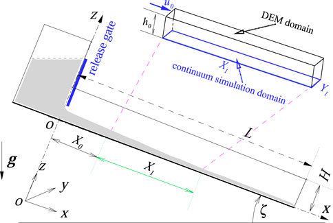
Figure 1. Schematic of the chute flow set-up. The Cartesian coordinate $(x,y,z)$ is aligned with the release gate, representing the downslope, cross-slope, upward normal directions, respectively. The DEM domain and continuum simulation domain are denoted in the top-right inset.

2.1.2 The CFD model

The CFD model for fluid flow adopts the volume-averaged Navier-Stokes equations, where the volume occupied by the fluid within each cell depends on the volume taken by the solid particles. Let ${\alpha }_f$ be the volume fraction, ${\mathit{u}}_f$ the fluid velocity, and ${\rho }_f$ the fluid density, the continuity equation of the CFD model can be given in Equation 3 as

$\frac{\partial }{\partial t}\left({\rho }_f{\alpha }_f\right)+\nabla \cdot \left({\rho }_f{\alpha }_f{\mathit{u}}_f\right)=0,(3)$

and the momentum Equation 4 is

$\frac{\partial }{\partial t}\left({\rho }_f{\alpha }_f{\mathit{u}}_f\right)+\nabla \cdot \left({\rho }_f{\alpha }_f{\mathit{u}}_f\otimes {\mathit{u}}_f\right)=-\nabla p+\nabla \cdot \left({\alpha }_f{\mathit{\tau }}_f\right)-{\mathit{F}}_{pf}+{\rho }_f{\alpha }_f\mathit{g},(4)$

where $\nabla p$ represents the pressure gradient, ${\tau }_f$ is fluid viscous stress tensor, ${\mathit{F}}_{pf}$ denotes the term associated with momentum transfer between the fluid and solid phase, $\mathit{g}$ is the vector of gravitational acceleration, and ‘$\cdot$’ represents the dot product while $\otimes$ denotes the dyadic product.

2.2 The depth-averaged granular flow model

The continuum simulation of chute flow is based on solving a depth-averaged granular flow model of the shallow water type (Stoker, 1957; Eglit and Shahinpoor, 1983; Savage and Hutter, 1989). By averaging the properties of the granular flow across the depth of the flow, this model reduces the computational complexity associated with simulating three-dimensional simulations. With the normal velocity component $w$ in the $z$ direction omitted, the mass and momentum equations of dimensionless form can be expressed as follows (Gray et al., 1999; Cui and Gray, 2013; Tregaskis et al., 2022).

$\frac{\partial h}{\partial t}+\nabla \cdot \left(h\bar{\mathit{u}}\right)=0,(5)$

$\begin{array}{ccc}\hfill \frac{\partial }{\partial t}\left(h\bar{\mathit{u}}\right)+\nabla \cdot \left(h\bar{\mathit{u}}\otimes \bar{\mathit{u}}\right)+\nabla \left(\frac{1}{2}g{h}^2\cos \zeta \right)& =\hfill & \mathit{S},\hfill \\ \hfill & \hfill & \hfill \end{array}(6)$

where $h$ is the flow thickness, $\bar{\mathit{u}}=(\bar{u},\bar{v})$ represents the velocity and its components in the $x$ and $y$ directions, respectively, and the gradient operator is $\nabla =(\partial /\partial x,\partial /\partial y)$. The source term $\mathit{S}=(S_x,S_y)$ on the right-hand side accounts for the effects of gravitational force and frictional resistance exerted on the basal surface, and is given in Equation 7 by

$\mathit{S}=gh\left(\mathit{i}\sin \zeta -\mu \left(\bar{\mathit{u}}/|\bar{\mathit{u}}|\right)\cos \zeta \right),(7)$

where $\mu =\tan \delta$ is the coefficient of friction with $\delta$ being the basal friction angle, $|\bar{\mathit{u}}|={\left({\bar{u}}^2+{\bar{v}}^2\right)}^{\frac{1}{2}}$, and $\mathit{i}$ is the unit vector in the $x-$direction.

Using the conservative variables $h$, $m=h\bar{u}$ and $n=h\bar{v}$, we can rewrite the system of Equations 5 and 6 into a non-strict hyperbolic form in Equations 8

$\frac{\partial \mathit{U}}{\partial t}+\frac{\partial \mathit{E}}{\partial x}+\frac{\partial \mathit{F}}{\partial y}=\mathit{S},(8)$

where $\mathit{U}={(h,m,n)}^T$ with the superscript $T$ denoting the transpose to a row vector. The respective fluxes and source term vector are given in Equation 9 below

$\begin{array}{c}\mathit{E}={\left(m,m^2/h+\frac{1}{2}g{h}^2\cos \zeta ,mn/h\right)}^T,\hfill \\ \mathit{F}={\left(n,mn/h,n^2/h+\frac{1}{2}g{h}^2\cos \zeta \right)}^T,\hfill \\ \mathit{S}={\left(0,S_x,S_y\right)}^T.\hfill \end{array}(9)$

To align with the dimensional DEM simulations, the following scaling is used: the length scale is set to $l=0.03$ meters, velocities are scaled by $\sqrt{gl}=0.54{\mathrm{m}\mathrm{s}}^{-1}$, and time is scaled by $\sqrt{l/g}=0.055$ seconds. Additionally, the Froude number $\text{Fr}$ is defined as the ratio of the flow speed $|\bar{\mathit{u}}|$ to the wave speed $c=\sqrt{h\cos \zeta }$, such that $\text{Fr}=|\bar{\mathit{u}}|/c$.

2.3 Implementation of the numerical simulations

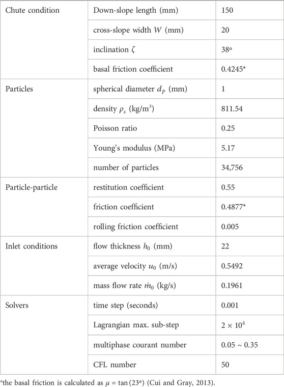
Without considering the complexity of the flow released from the hopper and gate, we focus our simulation on a region of the flow that is sufficiently developed along the slope of the chute. As shown in Figure 1, a typical chute flow set-up consists of a hopper, a release gate, and a chute with a bed and sidewalls. The chute has a downslope length $L$ (e.g., 1,000 mm), a cross-slope width $W$ (e.g., 300 mm), and an adjustable inclination $\zeta$ relative to the horizontal. The sidewalls of the chute are usually made of transparent material and have a height $H$ (e.g., 100 mm).Although our current focus is on numerical simulations, we follow the experimental setup for chute flows, such as described in Cui and Gray (2013); Cui et al. (2022), to define our computational domain. This alignment ensures that the initial flow thickness $h_0$ and velocity $u_0$ (e.g., obtained through high speed camera measurements using the particle image velocimetry (PIV) method) are well defined at a specific location in the chute. In Figure 1, this location is set at $x=X_0$ with the Cartesian coordinate $(x,y,z)$ aligned with the release gate. Such initial conditions are crucial for both DEM and continuum simulations. Consequently, the continuum simulation domain can be defined within a basal surface region with a downslope length of $X_1$ and a cross-slope width of $Y_1$, as illustrated in the top-right inset in Figure 1. In our case, we select $X_1=150$ mm and $Y_1=20$ mm, as no obstacles are used to divert the flow.

Following the selection of the simulation domain, the DEM simulation is conducted in a three-dimensional region where $x\in [\mathrm{0,150}]$ mm, $y\in [\mathrm{0,20}]$ mm, and $z\in [0,h_0]$ mm within the chute. The initial conditions are set $h_0=22$ mm and $u_0=0.5492$ m/s with an inclination angle $\zeta =38°$. This setup results in an initial mass flow rate of 0.1961 kg/s at the inlet. In the continuum simulation, the same initial conditions of $h_0$ and $u_0$ are applied. Key physical and control parameters used for the DEM simulation are summarized in Table 1.

Table 1

Table 1. Parameters and conditions used in the DEM simulation of chute flow.

The governing Equation 8 is solved numerically using a finite-difference method (Cui, 2014; Cui, 2021) on a uniform H-grid covering the domain defined by $x\in [\mathrm{0,150}]$ mm and $y\in [\mathrm{0,20}]$ mm. With a grid interval of 1 mm, the computational grid consists of $151\times 21$ points for the simulation. Due to the simplicity of the domain without obstacles, only the initial conditions of $h_0=22$ mm, ${\bar{u}}_0=0.5492$ m/s, and ${\bar{v}}_0=0$ m/s are needed at the upstream boundary. The other boundaries develop naturally as the flow propagates downstream. Since the numerical method is explicit, the time step is automatically controlled according to the CFL (Courant-Friedrichs-Lewy) stability condition (Anderson, 1995).Finally, the coupled CFD-DEM simulations were conducted using the Simcenter Star-CCM + package, and our continuum simulations utilized an in-house code developed for the finite difference method based on an explicit non-oscillatory central (NOC) scheme (Nessyahu and Tadmor, 1990).

3 DEM and continuum simulations of granular flow

3.1 Time-dependent development of the granular flow

Since DEM and continuum simulations are based on fundamentally different modeling frameworks in both spatial and temporal domains, it is particularly effective to first investigate the time-dependent development of the simulations. This approach provides an overall perspective, as well as a qualitative comparison, between the two methods. To achieve this, we simulate spherical particles with a diameter of 1 mm flowing down a 150 mm slope inclined at $\zeta =38°$.

As shown in Figure 2, the DEM solutions on the left-hand side generally agree well with the continuum solutions on the right-hand side, particularly at later stages of development, say, from $t=0.152$ seconds onward. Even at earlier times, such as $t=0.070$ and 0.1 s, the flow evolution is largely consistent between the DEM and continuum simulations. However, the results at $t=0.035$ seconds show an interesting difference, especially in the moving fronts. This discrepancy arises because, in the DEM simulation, a sheet of particles is injected at the inlet surface, and the particles then move down the slope in a solid-like state. In contrast, the continuum simulation produces a fluid-phase solution from the inlet, causing its moving front to become infinitely thin. Overall, due to mass conservation, the flow thickness decreases as its velocity increases while propagating further downslope.

Figure 2

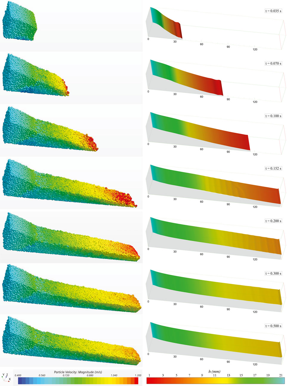
Figure 2. DEM and continuum simulations of time-dependent development in granular flow down a 150 mm by 20 mm slope.

3.2 Spatial-temporal averaged velocity and velocity profile

Figure 3 provides a more quantitative comparison for the spatial-temporal averaged downslope velocity <u>. This velocity is calculated during the simulation in a form of ${\sum }_{j=1}^{n_i}{u}_i/N$, where $u_i$ is the downslope velocity of a particle, $n_i$ is the temporal number of particles in the simulation, and $N$ represents the total number of particles in the steady-state solution. Normalizing <u> by $N$ allows its DEM solution to be directly comparable with the continuum solution, which is averaged over the entire computational domain–either the number of particles in the DEM steady-state solution (e.g., $N_{\text{dem}}=34756$) or grid points in the continuum simulation (e.g., $N_{\text{con}}=151\times 21=3171$). In this figure, both the DEM and continuum solutions converge to a steady state around the same time scale, approximately 0.25 s, though they exhibit notably different build-up histories. The figure also shows the steady-state downslope velocities obtained from the DEM solution at the free surface, mid-depth, and basal surface. The free-surface velocity aligns closely with the continuum solution, consistent with the granular flow being treated as a plug-flow type (Cui and Gray, 2013). On the other hand, the DEM solution at mid-depth closely matches the overall velocity profile, indicating a macroscopic representation of the particle velocities. Given that $N_{\text{dem}}$ and $N_{\text{con}}$ are completely independent measures of particle/grid details, the result in Figure 3 is particularly promising for assessing the microscopic and macroscopic behaviors.

Figure 3

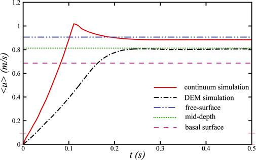
Figure 3. Time-dependent development of downslope velocity over a 150 mm slope: the solid line shows the depth-averaged continuum model result; the dash-dot line indicates the normalized DEM simulation velocity. The dash-dot-dot, dotted, and dashed lines represent the normalized velocities at the free surface, mid-depth, and basal surface, respectively.

A key advantage of continuum simulations over DEM simulations is their significantly lower computational cost. In our case, under similar computing conditions, the continuum simulation required only 42 s on a $151\times 21$ grid with a time step of 0.00055 s, whereas the DEM simulation took 8,750 s for up to 34,756 particles with an implicit time step of 0.001 s, both simulating up to 1 s of physical time. This demonstrates that the continuum simulation is over 200 times faster than the DEM. For a three-dimensional simulation, the continuum approach could still maintain a computational advantage, being approximately 10 times faster on a $151\times 21\times 23$ grid, with 23 grid points extended in the $z-$direction to cover a range of 22 mm $(=h_0)$.

Further details of velocities obtained from the DEM steady-state solution are shown in Figure 4. In this figure, the velocities have been averaged in the cross-slope $y$ direction to produce a velocity field, $<u^{\prime }>$ and $<w^{\prime }>$, in the downslope $x$ and normal $z$ directions, respectively. Since there is no obstacle in the flow field, the cross-slope velocity $v$ remains close to zero. In Figure 4A, the velocity field is overlaid with the magnitude of the velocity, showing a gradual increase from the basal surface at $z=0$ to the free surface. Also shown in Figure 4A is the steady-state free-surface height of the flow obtained from the continuum simulation, denoted in green circular symbols. The agreement of the free-surface heights between the DEM and continuum simulations is overly good, given the fact that these results are obtained independently, using only the same initial inlet conditions defined by $h_0$ and $u_0$ fogure 4b presents the velocity profiles along the flow thickness direction at various downslope locations $x=\mathrm{30,50},\dots ,150$ mm, obtained from the DEM simulation. Due to the “no-slip” viscous condition applied at the base of the slope, a significant velocity change is observed near the basal boundary, resembling a “boundary layer”. Beyond this layer, the velocity increases roughly linearly toward the free-surface. The corresponding depth-averaged velocity, $\bar{u}$, obtained from the continuum simulation is also shown in green circular symbols in Figure 4B. Since these velocities are based on the free-surface flow for a basal friction angle $\delta =23°$ where $\mu =\tan \delta$ (see, (7)), they closely match but are slightly higher than the free-surface solution of DEM. This may be generally expected in continuum simulations, as granular materials are assumed dry, cohesionless, and isotropic. By increasing the value of $\delta$ to $30°$, the continuum’s free-surface velocities align well with the DEM velocity profiles, as illustrated by white-filled circular symbols labelled $\delta =30°$ that cross the DEM profiles in Figure 4B (note, the vertical sense of $h$ has been discarded for this $\delta =30°$ case). In other words, analyzing velocity profiles of DEM can help better calibrate the basal friction coefficient, $\mu$, in continuum simulations, leading to a more consistent solution for granular flows.

Figure 4

Figure 4. Velocity profiles between the DEM and continuum simulations: (A) velocity field in the $x-z$ plane, overlaid by the free-surface thickness of the flow; (B) velocity distributions along the flow thickness direction at various downslope locations from the DEM simulation, compared with the depth-averaged velocity from the continuum simulation.

Accurately capturing the velocity profile is crucial for modelling the rheological behaviour of granular flows, particularly in continuum simulations (Pouliquen, 1999; GDR, 2004; Franci and Cremonesi, 2019; Tregaskis et al., 2022), while also serving as a metric for assessing the robustness and effectiveness of DEM simulations. As particle characteristics become more complex–such as in shape, size, moisture content, attrition, breakage, and mixing–modelling inter-particle contact and interaction becomes increasingly challenging (Guo and Curtis, 2015; Zhong et al., 2016; Vakis et al., 2018). However, detailed insights into particle velocity profiles are vital for uncovering critical physical insights into particle dynamics and behaviors. Since spherical particles represent the most typical shape, our results could offer a benchmark solution for further studies, including the application of machine learning.

4 Machine learning on the granular flow dataset

With the rapid advancement of computing technologies, artificial intelligence and machine learning are increasingly being applied to analyze fluid mechanics problems (Brunton et al., 2020; Molinaro et al., 2021). This section explores the use of machine learning techniques to analyze and interpret the granular flow dataset generated from the DEM simulations discussed in Section 3.1.

4.1 Machine learning framework

Using the Random Forest method as an example, we briefly explain how machine learning can be applied to granular flow data analysis (Breiman, 2001; Zaki and Meira, 2014; Clarke et al., 2009) from training, optimization, to prediction.

Let $\mathbf{X}=\{{\mathbf{x}}_1,{\mathbf{x}}_2,\dots ,{\mathbf{x}}_n\}$ be the input dataset, with each feature vector ${\mathbf{x}}_i={[x_{i1},x_{i2},\dots ,x_{im}]}^T$ in ${\mathbb{R}}^m$. In our case, the feature vector ${\mathbf{x}}_i$ can be defined to include particle-related information such as position, velocity, particle ID, forces, stresses, and volume fraction at each output time step from the DEM simulation. For example, if we use a time interval of 0.02 s over a total simulation time of 1 s, we would generate $\mathcal{N}=100$ feature vectors, forming the input (or training) dataset $\mathbf{X}$, stored in the space ${\mathbb{R}}^m$.

Let $\mathbf{Y}=\{y_1,y_2,\dots ,y_n\}$ represent the corresponding set of labels or target values, where $y_i\in \mathbb{R}$ for regression tasks. In this context, we test RandomForest, LinearRegression, and RidgeRegression models. The RandomForest model operates by building multiple decision trees, denoted by $T_j$, during training process and then aggregating their results to improve prediction accuracy. This can be expressed in Equation 10 as:

$\widehat{y}=\mathcal{F}\left(\mathbf{x}\right)=\frac{1}{B}{\displaystyle \sum _{j=1}^B}{T}_j\left(\mathbf{x}\right)(10)$

where $B$ is the total number of trees, $T_j(\mathbf{x})$ is the prediction from the $j$-th decision tree, and $\mathcal{F}(\mathbf{x})$ can be a generic machine learning model.

Consequently, a loss function, e.g., the Mean Squared Error (MSE), as given in Equation 11 as follows

$\mathcal{L}\left(\mathbf{Y},\widehat{\mathbf{Y}}\right)=\frac{1}{n}{\displaystyle \sum _{i=1}^n}{\left(y_i-{\widehat{y}}_i\right)}^2(11)$

can be used to measure the discrepancy between the true labels $\mathbf{Y}$ and the predicted labels $\widehat{\mathbf{Y}}$.

Without repeating further details of the training process (Breiman, 2001), the model is evaluated using a test dataset $({\mathbf{X}}_{\text{test}},{\mathbf{Y}}_{\text{test}})$. Metrics such as the $R^2$-score can be used to assess the model’s effectiveness, as demonstrated in Figure 5.

Figure 5

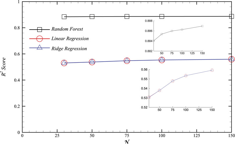
Figure 5. The $R^2$ scores versus the number of feature vectors $\mathcal{N}$ for the RandomForest, LinearRegression, and RidgeRegression methods in the machine learning of the granular flow dataset.

The trained RandomForest model is then applied to predict outputs for new, unseen data points ${\mathbf{x}}_{\text{new}}$, using Equation 12:

${\widehat{y}}_{\text{new}}=\frac{1}{B}{\displaystyle \sum _{j=1}^B}{T}_j\left({\mathbf{x}}_{\text{new}}\right).(12)$

4.2 Implementation of the machine learning method

When training a machine learning model, it is essential to split the dataset $(\mathbf{X},\mathbf{Y})$ into a training set $({\mathbf{X}}_{\text{train}},{\mathbf{Y}}_{\text{train}})$ and a test set $({\mathbf{X}}_{\text{test}},{\mathbf{Y}}_{\text{test}})$. Typically, around $80\%$ of the data is allocated to training, while the remaining $20\%$ is reserved for testing. This split allows the model to learn patterns from the training data and then assess its performance on the test data to evaluate how well it has generalized those patterns, which can be measured by the $R^2$-score for the loss function (11).

In Figure 5, three machine learning models–RandomForest, LinearRegression, and RidgeRegression–are used to train the granular flow dataset with different numbers of feature vectors at $\mathcal{N}=\mathrm{30,50,75,100,150}$. Notably, the RandomForest model consistently outperforms both the Linear and Ridge regression models, which rely on fitting a linear relation to the observed model. Additionally, increasing the number of feature vectors $\mathcal{N}$ does not appear to significantly improve the model scores.

Figure 6 shows the predicted output, ${\widehat{y}}_{\text{new}}$, generated by the Random Forest, Ridge Regression, and Linear Regression models for the granular flow dataset. In this case, the models are used to predict particle positions. The images in the top panel, (a) and (b), are drawn from the test data and represent the true steady-state solution of DEM, as shown in Figure 2 e.g., at $t=0.5$ seconds. The corresponding predictions by the Random Forest model are shown in Figures 6C, D, by the Ridge Regression model in (e) and (f), and by the Linear Regression in (g) and (h), respectively. The images on the left (a,c,e,g) and right (b,d,f,h) panels show the same result from different viewing angles.

Figure 6

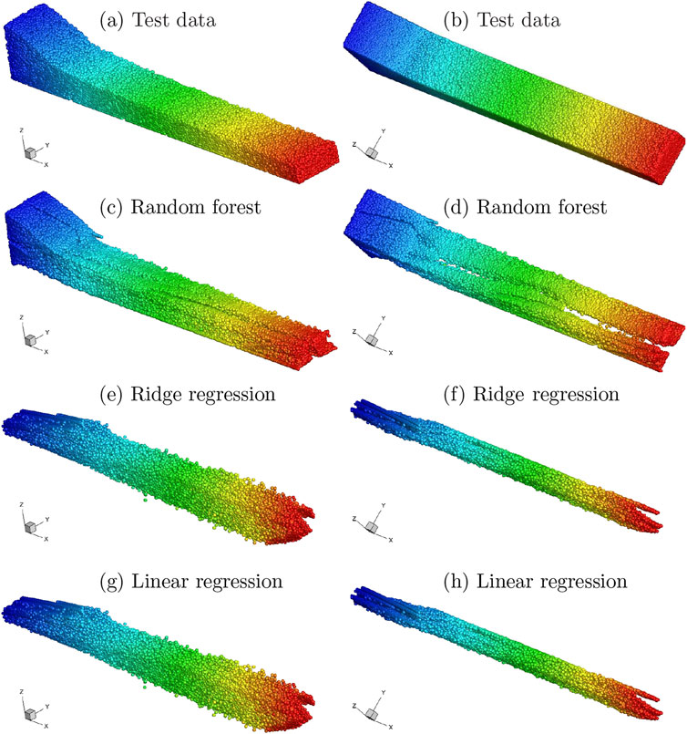
Figure 6. Random Forest, Ridge Regression and Linear Regression machine learning applied to the granular flow dataset, with a comparison to the “true” flow pattern in the test data. (A, B) Test data (C) Random forest (D) Random forest (E) Ridge regression (F) Ridge regression (G) Linear regression (H) Linear regression

Even with the RandomForest model, the predicted result shows a significant discrepancy from the true solution, highlighting the challenges of applying machine learning to accurately predict even relatively simple granular flow patterns. One possible reason for this disagreement is that the original training dataset was selected from the initial injection phase of the flow through to its steady state. This may have complicated (deliberately) the training process due to the continuously evolving flow patterns, as seen in Figure 2. Nevertheless, there is ongoing development in machine learning techniques to address such complexities, with methods like physics-informed neural networks (PINNs) (Karniadakis et al., 2021; Wang et al., 2021; Mao et al., 2020) and graph neural networks (GNNs) (Choi and Kumar, 2024) being tested for tackling complex fluid mechanics problems.

5 Conclusions and recommendations

In this study, we investigated the dynamics of granular flow using both Discrete Element Method (DEM) and continuum modeling, providing an insight to the micro-scale interactions and macro-scale behavior of granular materials. The comparative analysis revealed that although both methods produced generally consistent results, discrepancies, particularly in early-stage flow development, underscore the complexity of accurately simulating granular materials. Furthermore, we explored the application of machine learning techniques, including Random Forest, Ridge Regression, and Linear Regression models, to predict particle positions within the granular flow. While the Random Forest model outperformed the linear models, the overall prediction accuracy highlighted the inherent challenges in using machine learning for complex granular systems.

While the use of spherical particle shapes provides robustness in DEM simulations, actual particle conditions are often more complex, especially in food processing applications.These factors may impose significant complexity to understanding granular particle behaviors. As illustrate in Figure 7, particle size and shape, even for spheres and capsules, can substantially influence particle packing condition, measured by the volume fraction. Within the moving flow mass, particles tend to segregate noticeably based on volume fraction. On the other hand, food particles frequently exhibit varying properties across seasons and regions, making it further challenging to accurately model and simulate their behavior due to the limited knowledge of their complex compositions (Vakis et al., 2018; Fries, 2021). Further exploration in the field of contact mechanics, fracture mechanics, and tribology is therefore essential for more realistically modeling particle interactions at the microscopic scale. Similarly, improvements in granular process rheology are needed to more accurately capture macroscopic flow behaviors (Dunatunga and Kamrin, 2015; Krishnaraj and Nott, 2015). These remain some of the most demanding tasks in the modeling and simulation of granular food processes.

Figure 7

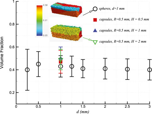
Figure 7. Size and shape on the volume fraction (with error bars) of granular particles, and $d$ is the diameter of spherical particles.

Using the rice milling process as an example, it involves several mechanical processes that exert various forces on the grain, significantly influencing the extent of breakage (Einav, 2007). Particle breakage under impact conditions is often modeled by considering energy dissipation, material resistance, and energy efficiency (Vogel and Peukert, 2003; Shitanda et al., 2001), and DEM-PBM (particle balance method) simulations have been tested for this purpose (Han et al., 2016; Metta et al., 2018; Cabiscol et al., 2021; Nakamura et al., 2022). Additionally, the Material Point Method (MPM) has been introduced in continuum modeling to allow granular materials to transition through various phases during the flow process (Dunatunga and Kamrin, 2015; Haeri and Skonieczny, 2022).

Given the challenges faced by traditional machine learning models in predicting granular flow patterns, future efforts should explore advanced techniques, such as physics-informed neural networks (PINNs) and graph neural networks (GNNs) (Cai et al., 2020; Choi and Kumar, 2024). These methods, which integrate physical laws and complex network structures, could offer more accurate predictions by better capturing the inherent dynamics of granular materials.

Finally, continuous validation of simulation results against experimental data is crucial for ensuring the reliability of both DEM and continuum models. Establishing benchmark cases, particularly for spherical particles, as presented in this study, can provide a valuable reference for future research, enabling the comparison and improvement of various modeling approaches.

Data availability statement

The original contributions presented in the study are included in the article/supplementary material, further inquiries can be directed to the corresponding author.

Author contributions

XC: Conceptualization, Methodology, Supervision, Writing–original draft, Writing–review and editing. DA: Data curation, Investigation, Software, Writing–original draft, Writing–review and editing. HZ: Conceptualization, Project administration, Resources, Writing–review and editing. MH: Conceptualization, Project administration, Resources, Writing–review and editing. AA: Conceptualization, Project administration, Resources, Writing–review and editing. TO: Investigation, Writing–review and editing. KS: Investigation, Writing–review and editing. SF: Investigation, Writing–review and editing.

Funding

The author(s) declare that financial support was received for the research, authorship, and/or publication of this article. The authors would like to acknowledge the support of the Innovate United Kingdom grant BB/S020993, EPSRC Grant EP/V521140/1, the Royal Society grant SIF/R2/212009, and Innovate United Kingdom Grant 10075111 for conducting this research.

Acknowledgments

Xinjun Cui is a Royal Society Short Industry Fellow. For the purpose of open access, the authors have applied a Creative Commons Attribution (CC BY) licence to any Author Accepted Manuscript version arising from this submission.

Conflict of interest

Author AA was employed by Koolmill Systems Ltd.

The remaining authors declare that the research was conducted in the absence of any commercial or financial relationships that could be construed as a potential conflict of interest.

Publisher’s note

All claims expressed in this article are solely those of the authors and do not necessarily represent those of their affiliated organizations, or those of the publisher, the editors and the reviewers. Any product that may be evaluated in this article, or claim that may be made by its manufacturer, is not guaranteed or endorsed by the publisher.

References

Amarsid, L., Delenne, J. Y., Mutabaruka, P., Monerie, Y., Perales, F., and Radjai, F. (2017). Viscoinertial regime of immersed granular flows. Phys. Rev. E 96, 012901. doi:10.1103/PhysRevE.96.012901

PubMed Abstract | CrossRef Full Text | Google Scholar

Anderson, J. D. (1995). Computational fluid dynamics. McGraw-Hill.

Google Scholar

Bérard, A., Patience, G. S., and Blais, B. (2020). Experimental methods in chemical engineering: unresolved CFD-DEM. Can. J. Chem. Eng. 98, 424–440. doi:10.1002/cjce.23686

CrossRef Full Text | Google Scholar

Boyer, F., Guazzelli, É., and Pouliquen, O. (2011). Unifying suspension and granular rheology. Phys. Rev. Lett. 107, 188301. doi:10.1103/PhysRevLett.107.188301

PubMed Abstract | CrossRef Full Text | Google Scholar

Breiman, L. (2001). Random forest. Mach. Learn. 45, 5–32. doi:10.1023/a:1010933404324

CrossRef Full Text | Google Scholar

Brunton, S. L., Noack, B. R., and Koumoustakos, P. (2020). Machine learning for fluid mechanics. Annu. Rev. Fluid Mech. 52, 477–508. doi:10.1146/annurev-fluid-010719-060214

CrossRef Full Text | Google Scholar

Cabiscol, R., Finke, J. H., and Kwade, A. (2021). A bi-directional DEM-PBM coupling to evaluate chipping and abrasion of pharmaceutical tablets. Adv. Powder Technol. 32, 2839–2855. doi:10.1016/j.apt.2021.06.002

CrossRef Full Text | Google Scholar

Cai, S., Mao, Z., Wang, Z., Yin, M., and Karniadakis, G. E. (2020). Physics-informed neural network (PINNs) for fluid mechanics: a review. Acta Mech. Sinca 37, 7127–1738. doi:10.48550/arXiv.2105.09506

CrossRef Full Text | Google Scholar

Choi, Y., and Kumar, K. (2024). Graph neural network-based surrogate model for granular flows. Comput. Geotech. 166, 106015. doi:10.1016/j.compgeo.2023.106015

CrossRef Full Text | Google Scholar

Clarke, B., Fokoué, E., and Zhang, H. (2009). Principles and theory for data mining and machine learning. Springer.

Google Scholar

Crowe, C. T., Sommerfeld, M., and Tsuji, Y. (2012). Multiphase flows with droplets and particles, 2nd Ed. Boca Raton, (CRC Press)

Google Scholar

Cui, K. F. E., Zhou, G. D., Jing, L., Chen, X., and Song, D. (2020). Generalized friction and dilatancy laws for immersed granular flows consisting of large and small particles. Phys. Fluids 32, 113312. doi:10.1063/5.0024762

CrossRef Full Text | Google Scholar

Cui, X. (2014). Computational and experimental studies of rapid free-surface granular flows around obstacles. Comput. & Fluids 89, 179–190. doi:10.1016/j.compfluid.2013.10.036

CrossRef Full Text | Google Scholar

Cui, X. (2021). Strong oblique shock waves in granular free-surface flows. Phys. Fluids 33, 0833024. doi:10.1063/5.0057700

CrossRef Full Text | Google Scholar

Cui, X., and Gray, J. M. N. T. (2013). Gravity-driven granular free-surface flow around a circular cylinder. J. Fluid Mech. 720, 314–337. doi:10.1017/jfm.2013.42

CrossRef Full Text | Google Scholar

Cui, X., Harris, M., Howarth, M., Zealey, D., Brown, R., and Shepherd, J. (2022). Granular flow around a cylindrical obstacle in an inclined chute. Phys. Fluids 34, 093308. doi:10.1063/5.0101694

CrossRef Full Text | Google Scholar

Cundall, P. A., and Strack, O. D. L. (1979). A discrete numerical model for granular assemblies. Geotechnique 29 (1), 47–65. doi:10.1680/geot.1979.29.1.47

CrossRef Full Text | Google Scholar

Dhiman, A., and Prabhakar, P. K. (2021). Micronization in food processing: a comprehensive review of mechanistic approach, physicochemical, functional properties and self-stability of micronized food materials. J. Food Eng. 292, 110248. doi:10.1016/j.jfoodeng.2020.110248

CrossRef Full Text | Google Scholar

Dunatunga, S., and Kamrin, K. (2015). Continuum modelling and simulation of granular flows through their many phases. J. Fluid Mech. 779, 483–513. doi:10.1017/jfm.2015.383

CrossRef Full Text | Google Scholar

Eglit, M. E. (1983). “Some mathematical models of snow avalanches,”. Advances in mechanics and the flow of granular materials. Editor M. Shahinpoor (Clausthal-Zellerfeld: Gulf Publishing Company), 2, 577–588.

Google Scholar

Einav, I. (2007). Breakage mechanics-Part II: modelling granular materials. J. Mech. Phys. 55 (6), 1298–1320. doi:10.1016/j.jmps.2006.11.004

CrossRef Full Text | Google Scholar

Forterre, Y., and Pouliquen, O. (2008). Flows of dense granular media. Annu. Rev. Fluid Mech. 40, 1–24. doi:10.1146/annurev.fluid.40.111406.102142

CrossRef Full Text | Google Scholar

Franci, A., and Cremonesi, M. (2019). 3D regularized (I) rheology for granular flows simulation. J. Comput. Phys. 378, 257–277. doi:10.1016/j.jcp.2018.11.011

CrossRef Full Text | Google Scholar

Fries, L. (2021). Modeling food particle systems: a review of current progress and challenges. Annu. Rev. Chem. Biomol. Eng. 12, 97–113. doi:10.1146/annurev-chembioeng-121820-081524

PubMed Abstract | CrossRef Full Text | Google Scholar

Gdr, M. (2004). On dense granular flows. Eur. Phys. J. E 14, 341–365. doi:10.1140/epje/i2003-10153-0

PubMed Abstract | CrossRef Full Text | Google Scholar

Gray, J. M. N. T. (2018). Particle segregation in dense granular flows. Annu. Rev. Fluid Mech. 50, 407–433. doi:10.1146/annurev-fluid-122316-045201

CrossRef Full Text | Google Scholar

Gray, J. M. N. T., Wieland, M., and Hutter, K. (1999). Gravity-driven free surface flow of granular avalanches over complex basal topography. Proc. Roy. Soc. A 455, 1841–1874. doi:10.1098/rspa.1999.0383

CrossRef Full Text | Google Scholar

Guo, Y., and Curtis, J. S. (2015). Discrete element method simulations for complex granular flows. Annu. Rev. Fluid Mech. 47, 21–46. doi:10.1146/annurev-fluid-010814-014644

CrossRef Full Text | Google Scholar

Haeri, A., and Skonieczny, K. (2022). Three-dimensionsal granular flow continuum modeling via material point method with hyperelastic nonlocal granular fluidity. Comput. Methods Appl. Mech. Engrg. 394, 114904. doi:10.1016/j.cma.2022.114904

CrossRef Full Text | Google Scholar

Han, Y., Jia, F., Zeng, Y., Jiang, L., Zhang, Y., and Cao, B. (2016). Effects of rotation speed and outlet opening on particle flow in a vertical rice mill. Powder Technol. 297, 153–164. doi:10.1016/j.powtec.2016.04.022

CrossRef Full Text | Google Scholar

He, K., Shi, H., and Yu, X. (2022). Effects of interstitial water on collapses of partially immersed granular columns. Phys. Fluids 34, 023306. doi:10.1063/5.0079468

CrossRef Full Text | Google Scholar

Johnson, K. L. (1987). Contact mechanics. Cambridge: Cambridge University Press.

Google Scholar

Kamrin, K., Hill, K. M., Goldman, D. I., and Andrade, J. E. (2024). Advances in modeling dense granular media. Annu. Rev. Fluid Mech. 56, 215–240. doi:10.1146/annurev-fluid-121021-022045

CrossRef Full Text | Google Scholar

Karniadakis, G. E., Kevrekidis, I. G., Lu, L., Perdikaris, P., Wang, S., and Yang, L. (2021). Physics-informed machine learning. Nat. Rev. Phys. 3, 422–440. doi:10.1038/s42254-021-00314-5

CrossRef Full Text | Google Scholar

Kieckhefen, P., Pietsch, S., Dosta, M., and Heinrich, S. (2020). Possibilities and limits of computational fluid dynamics - discrete element method simulations in process engineering: a review of recent advancements and future trends. Annu. Rev. Chem. Biomol. Eng. 11, 397–422. doi:10.1146/annurev-chembioeng-110519-075414

PubMed Abstract | CrossRef Full Text | Google Scholar

Krishnaraj, K. P., and Nott, P. R. (2015). A dilation-driven vortex flow in sheared granular materials explains a rheometric anomaly. Nat. comms 7, 10630. doi:10.1038/ncomms10630

PubMed Abstract | CrossRef Full Text | Google Scholar

Li, T., Zhang, H., Kuang, S., Yan, H., Diao, X., Huang, Z., et al. (2020). Experimental and numerical study of coarse particle conveying in the small absorber sphere system: overview and some recent CFD-DEM simulations. Nucl. Eng. Des. 357, 110420. doi:10.1016/j.nucengdes.2019.110420

CrossRef Full Text | Google Scholar

Ma, G., Guan, S., Wang, Q., Feng, Y. T., and Zhou, W. (2022). A predictive deep learning framework for path-dependent mechanical behavior of granular materials. Acta Geotech. 17, 3463–3478. doi:10.1007/s11440-021-01419-y

CrossRef Full Text | Google Scholar

Mao, Z., Jagtap, A. D., and Karniadakis, G. E. (2020). Physics-informed neural networks for high-speed flows. Comput. Methods Appl. Mech. Engrg. 360, 112789. doi:10.1016/j.cma.2019.112789

CrossRef Full Text | Google Scholar

Metta, N., Ierapetritou, M., and Ramachandran, R. (2018). A multiscale DEM-PBM approach for a continuous comilling process using a mechanistically developed breakage kernel. Chem. Eng. Sci. 178, 211–221. doi:10.1016/j.ces.2017.12.016

CrossRef Full Text | Google Scholar

Molinaro, R., Singh, J., Catsoulis, S., Narayanan, C., and Lakehal, D. (2021). Embedding data analytics and CFD into the digital twin concept. Comput. Fluids 214, 104759. doi:10.1016/j.compfluid.2020.104759

CrossRef Full Text | Google Scholar

Muntán, E., García, C., Oller, P., Martí, G., García, A., and Gutiérrez, E. (2009). Reconstructing snow avalanche in the southeastern pyrenees. Nat. Hazard Earth Syst. Sci. 9, 159901612. doi:10.5194/nhess-9-1599-2009

CrossRef Full Text | Google Scholar

Nakamura, H., Baba, T., Ohsaki, S., Watano, S., Takehara, K., and Higuchi, T. (2022). Numerical simulation of wet granulation using the DEM-PBM coupling method with a deterministically calculated agglomeration kernel. Chem. Eng. J. 450, 138298. doi:10.1016/j.cej.2022.138298

CrossRef Full Text | Google Scholar

Nessyahu, H., and Tadmor, E. (1990). Non-oscillatory central differencing for hyperbolic conservation laws. J. Comput. Phys. 87, 408–463. doi:10.1016/0021-9991(90)90260-8

CrossRef Full Text | Google Scholar

Pouliquen, O. (1999). Scaling laws in granular flows down rough inclined planes. Phys. Fluids 11 (3), 542–548. doi:10.1063/1.869928

CrossRef Full Text | Google Scholar

Raissi, M., Yazdani, A., and Karniadakis, G. E. (2020). Hidden fluid mechanics: learning velocity and pressure fields from flow visualizations. Science 367, 1026–1030. doi:10.1126/science.aaw4741

PubMed Abstract | CrossRef Full Text | Google Scholar

Renzo, A. D., and Maio, F. P. D. (2004). Comparison of contact-force models for the simulation of collisions in DEM-based granular flow codes. Chem. Eng. Sci. 59, 525–541. doi:10.1016/j.ces.2003.09.037

CrossRef Full Text | Google Scholar

Savage, S. B., and Hutter, K. (1989). The motion of a finite mass of granular material down a rough incline. J. Fluid Mech. 199, 177–215. doi:10.1017/s0022112089000340

CrossRef Full Text | Google Scholar

Sen, O., Gaul, N. J., Choi, K. K., Jacobs, G., and Udaykumar, H. S. (2018). Evaluation of multifidelity surrogate modeling techniques to construct closure laws for drag in shock–particle interactions. J. Comput. Phys. 371, 434–451. doi:10.1016/j.jcp.2018.05.039

CrossRef Full Text | Google Scholar

Shitanda, D., Nishiyama, Y., and Koide, S. (2001). Performance analysis of impeller and rubber roll husker using different variaties of rice. Agri. Eng. Int. CIGR J. 19.

Google Scholar

Si, P., Shi, H., and Yu, X. (2018). Development of a mathematical model for submarine granular flows. Phys. Fluids 30, 083302. doi:10.1063/1.5030349

CrossRef Full Text | Google Scholar

Stoker, J. T. (1957). Water waves. Elsevier.

Google Scholar

Tregaskis, C., Johnshon, C. G., Cui, X., and Gray, J. M. N. T. (2022). Subscritical and supercritical granular flow around an obstacle on a rough inclined plane. J. Fluid Mech. 933, A25-1–A25-41. doi:10.1017/jfm.2021.1074

CrossRef Full Text | Google Scholar

Vakis, A. I., Yastrebov, V. S., Scheibert, J., Nicola, L., Dini, D., Ciavarella, M., et al. (2018). Modelling and simulation in tribology across scales: an overview. Tribol. Int. 125, 169–199. doi:10.1016/j.triboint.2018.02.005

CrossRef Full Text | Google Scholar

Vijayan, A., Baju, J., and Kumar, A. R. (2021). Fluid flow assisted mixing of binary granular beds using CFD-DEM. Powder Technol. 383, 183–197. doi:10.1016/j.powtec.2021.01.040

CrossRef Full Text | Google Scholar

Vogel, L., and Peukert, W. (2003). Breakage behaviour of different materials-construction of a mastercurve for the breakage probability. Powder Technol. 129, 101–110. doi:10.1016/s0032-5910(02)00217-6

CrossRef Full Text | Google Scholar

Wang, K., Che, Y., Mehana, M., Lubbers, N., Bennet, K. C., Kang, Q., et al. (2021). A physics-informed and hierarchically regularized data-drive model for predicting fluid flow through porous media. J. Comput. Phys. 445, 110526. doi:10.1016/j.jcp.2021.110526

CrossRef Full Text | Google Scholar

Zaki, M. J., and Meira, W. (2014). Data mining and analysis: fundamental concepts and algorithms. Cambridge University Press.

Google Scholar

Zhao, J., Zhao, S., and Luding, S. (2023). The role of particle shape in computational modelling of granular matter. Nat. Rev. Phys. 5, 505–525. doi:10.1038/s42254-023-00617-9

CrossRef Full Text | Google Scholar

Zhong, W., Yu, A., Liu, X., Tong, Z., and Zhang, H. (2016). DEM/CFD-DEM modelling of non-spherical particulate systems: theoretical developments and applications. Powder Technol. 302, 108–152. doi:10.1016/j.powtec.2016.07.010

CrossRef Full Text | Google Scholar