Comparison of machine learning methods for predicting ground-level ozone pollution in Beijing

High ground - level ozone (O₃) concentrations severely undermine urban air quality and threaten human health, creating an urgent need for precise and effective ozone - level predictions to aid environmental monitoring and policy - making.This study incorporated the historical concentrations of ozone and nitrogen dioxide (NO₂) from the past 3 hours as lagged features into a Lagged Feature Prediction Model (LFPM), evaluated using nine machine - learning algorithms (including XGBoost). Initially, XGBoost combined with SHAP identified 11 key features, boosting computational efficiency by 30% without sacrificing prediction accuracy. Then, ozone concentrations were predicted using six meteorological variables.Results showed that LSTM - based methods, especially ED - LSTM, performed best among meteorological - only models (R² = 0.479). Yet, predictions based solely on meteorological variables had limited accuracy. Adding five pollutant variables markedly improved the predictive performance across all machine - learning methods. XGBoost achieved the highest accuracy (R² = 0.767, RMSE = 11.35 μg/m³), a 125% relative improvement in R² compared to meteorological - variable - only predictions. Further application of the LFPM model enhanced prediction accuracy for all nine machine - learning methods, with XGBoost still leading (R² = 0.873, RMSE = 8.17 μg/m³).These findings conclusively demonstrate that integrating lagged feature variables significantly enhances ozone prediction accuracy, offering stronger support for environmental monitoring and policy - formulation.

1 Introduction

With the accelerating pace of urbanization, air pollution has emerged as a critical global challenge, where ozone (O₃) concentration dynamics have become a pivotal indicator of atmospheric quality (Ellingsen et al., 2008; Li et al., 2019). As a secondary pollutant formed through complex photochemical processes, O₃ levels exhibit strong dependencies on meteorological parameters, vehicular emissions, and industrial activities (Suciu et al., 2017; Wang et al., 2017; Tan et al., 2022). While stratospheric ozone serves as a protective shield against ultraviolet radiation, elevated ground-level ozone concentrations demonstrate profound detrimental effects: epidemiological studies directly associate chronic exposure with respiratory morbidity (e.g., asthma exacerbation) and ocular damage at peak concentrations (Li, 2020b; Maji and Namdeo, 2021; Zheng et al., 2021; Niu, 2022). Furthermore, O₃ phytotoxicity induces leaf chlorosis and stomal dysfunction, ultimately driving agricultural yield reduction–a growing concern for food security (Emberson, 2020; Peng et al., 2020). These multifaceted impacts underscore the urgency of ozone pollution mitigation. Mechanistically, tropospheric O₃ generation primarily stems from sunlight-driven reactions between nitrogen oxides (NO_x) and volatile organic compounds (VOC_s) (Bais et al., 2015; Monks et al., 2015; Wang et al., 2023). The complexity of these photochemical reactions, coupled with their pronounced spatiotemporal variability, poses substantial obstacles in developing reliable predictive models and effective control strategies.

Current research on ozone pollution prediction primarily employs deterministic and statistical approaches. Deterministic methods, such as process-based numerical modeling systems, require explicit parameterization of intricate physicochemical mechanisms. These models often face challenges including prohibitive computational costs and uncertainties stemming from emission inventories and parameterization schemes (Sun et al., 2021; Yang and Zhao, 2023). Conversely, traditional statistical techniques like linear regression can identify linear correlations between predictors and ozone levels but fail to resolve the complex nonlinear couplings between O₃, its precursors (NO_x and VOC_s), and meteorological drivers, leading to compromised predictive accuracy (Comrie, 1997; Zhou et al., 2023). In contrast, machine learning (ML) approaches exhibit superior capability in modeling such nonlinear interactions while maintaining computational efficiency, effectively overcoming the limitations of conventional methods. Distinct from physics-based frameworks, ML operates within a non-parametric paradigm, eliminating dependence on a priori assumptions about data distributions. By autonomously extracting discriminative features from multidimensional datasets through explicit learning mechanisms, ML has garnered substantial research attention in recent years for pollution forecasting applications (Mallet et al., 2009; Zhu et al., 2024).

Recent advancements in ML have revolutionized ozone concentration modeling, particularly demonstrating exceptional efficacy in localized regional applications. Empirical evidence increasingly substantiates ML algorithms’ capability to precisely simulate ground-level ozone dynamics, with state-of-the-art models consistently achieving superior predictive performance (R² > 0.8 in most implementations). Notably, spatial implementations showcase remarkable success: In the Beijing-Tianjin-Hebei megacity cluster, (Ma et al., 2021), developed a Random Forest (RF)-based prediction framework achieving robust predictive performance (R² = 0.85), effectively capturing regional transport patterns. At national scale, (Li et al., 2020), employed Gradient Boosting Regression Trees (GBRT) for China-wide ozone simulation, demonstrating exceptional generalizability through ten-fold cross-validation (R² = 0.89). Regional refinement was exemplified by (Yang et al., 2024), whose RF implementation in the topographically complex Sichuan Basin yielded an R² of 0.87, outperforming conventional chemical transport models. Seasonal predictability was further verified by (Chen et al., 2024) through comparative analysis of 4 ML algorithms in the Pearl River Delta’s autumn ozone episodes, identifying Support Vector Regression (SVR) as optimal (R² = 0.88).

Emerging methodological innovations further demonstrate ML’s transformative potential in ozone prediction (Cheng et al., 2022). pioneered a hybrid architecture integrating Variational Autoencoders (VAE) with Generative Adversarial Networks (GAN), achieving sub-minute temporal resolution (hourly predictions) without compromising accuracy - a critical advancement for real-time monitoring systems. Comparative analysis by Du et al. (2022) across decade-long Houston ozone datasets (2010–2020) identified XGBoost as the optimal algorithm, outperforming conventional approaches in capturing emission trend interactions. Region-specific adaptations have proven particularly effective in tropical environments (Dhanya et al., 2022). synergized meteorological parameters with Principal Component Analysis (PCA)-enhanced Artificial Neural Networks (ANN) for South Bangalore, India, demonstrating comparable efficacy between standalone ANN and PCA-ANN frameworks (R² > 0.82). Conversely, integrated modeling paradigms combining multi-source data reveal fundamental chemical regime transitions (Wang et al., 2019). reconciled satellite retrievals, in-situ measurements, and regional chemical transport modeling to decode ozone-precursor relationships, identifying a widespread shift from VOC-sensitive to NOx-sensitive O₃ formation mechanisms - though notable regional exceptions necessitate location-specific control strategies. Notwithstanding their mechanistic insights, purely physics-based numerical models face inherent limitations: excessive computational resource requirements, dependency on error-prone emission inventories, and specialized operational expertise create substantial implementation barriers for widespread policymaking applications.

Although machine learning techniques have been widely applied to ozone pollution prediction, existing studies have mainly focused on optimizing model structures, with limited systematic evaluations of feature engineering, especially lag features (i.e., using historical data to construct input variables) across different time scales. Considering that ozone concentration is influenced by the accumulation effect of precursor pollutants and meteorological conditions with time lags, this study proposes a prediction model that integrates different lag feature variables (LFPM). This model constructs feature variables by combining historical ozone (1–3 h) and nitrogen dioxide (1–3 h) observation data and systematically evaluates its prediction performance based on nine machine learning methods, including XGBoost, Random Forest, LSTM, and others, covering tree models, neural networks, and traditional regression methods.

Unlike previous studies that typically compare only two to three models, this study analyzes prediction accuracy, computational efficiency, model robustness, and other aspects, and further explores the variation in prediction accuracy of each model for forecasting the next 24 h. Through multi-model comparative experiments, we propose an optimal lag feature selection scheme for urban ozone pollution prediction and validate it using real-world pollution data from Beijing to improve the model’s generalization ability and practical application value.

The results of this study not only provide theoretical support for the optimization of machine learning models in ozone prediction but also offer empirical evidence for optimizing feature engineering and decision-making in air quality early warning systems, thereby enhancing the interpretability and practical value of the models.

2 Materials and methods

2.1 Study data and experimental procedures

This study aims to achieve two objectives: (1) systematically compare the performance differences of nine machine learning models (including XGBoost, Random Forest, LSTM, etc.) in predicting hourly ozone concentrations, with a focus on evaluating their prediction accuracy (R², RMSE, MAE) and computational efficiency (training time, single prediction time); (2) based on this, construct a lag feature prediction model (LFPM) that integrates various historical pollution observation data, optimizing the feature space by introducing time-lagged variables (such as pollutant concentrations from the previous 1–3 h), and explore the impact of feature engineering on model performance, while further comparing and observing the prediction accuracy of each model at different prediction time scales (the next 24 h).

Specifically, the experimental design uses a set of standard pollutant and meteorological data to build ozone prediction models with nine machine learning methods, aiming to predict the ozone concentration at the next time step, i.e., the next hour. Feature selection is performed to reduce the training dataset and improve model efficiency, ultimately selecting the six most important pollutant variables and five meteorological variables. To optimize the performance of each method, we use the GridSearchCV function from the Python Sklearn library for hyperparameter tuning. Additionally, in the hyperparameter tuning process, to prevent data leakage and ensure model consistency with time series data, we adopt the TimeSeriesSplit (5-fold cross-validation) method. This approach progressively expands the training window while maintaining the time order, using subsequent data as a validation set to simulate the data usage in real-world prediction tasks.

This study utilizes high-temporal-resolution pollutant monitoring data and meteorological reanalysis datasets spanning January 1 to 31 December 2023. The hourly ground-level air quality observations were obtained from Station 1006A (41°32′35″N, 116°35′32″E) of the China National Environmental Monitoring Center (CNEMC) network (https://www.cnemc.cn/), representing a typical urban background monitoring site. Meteorological inputs were derived from the ERA5-Land reanalysis product (ECMWF) with 0.25 ° × 0.25 ° spatial resolution and hourly temporal resolution. Site-specific meteorological parameters were extracted through bilinear interpolation centered on the station coordinates (41°32′35″N, 116°35′32″E), ensuring spatiotemporal alignment with pollutant measurements.

Missing values and outliers in the pollutant and meteorological data may be caused by factors such as sensor malfunctions. Therefore, data cleaning is required before building machine learning models. To handle missing values in the pollutant observation data and meteorological data, a unified interpolation method was used. To better accommodate the characteristics of time series data, the rolling mean interpolation method was applied for missing values, which more accurately reflects the temporal and continuity nature of the data. For handling outliers, the median substitution method was chosen. The median effectively suppresses the impact of outliers on the data distribution, avoiding bias that could be caused by extreme values. It is important to note that, during interpolation, some missing values are not just missing data but may result from missing data points at corresponding times, which could lead to errors in interpolation. Therefore, before interpolation, missing time points were first supplemented to ensure that the interpolation process could generate continuous time series data. To simplify the expression, the variable names used in the model were abbreviated (Table 1). All data processing steps were ultimately consolidated into a single CSV file and processed using Python’s Pandas library (Figure 1). The model’s performance was evaluated by calculating the error metrics between the predicted ozone concentration and the actual observed concentration 1 hour later.

Table 1

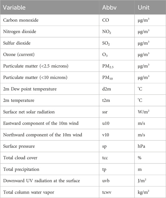
Table 1. List of parameters for meteorological and pollutant variables used in this study.

Figure 1

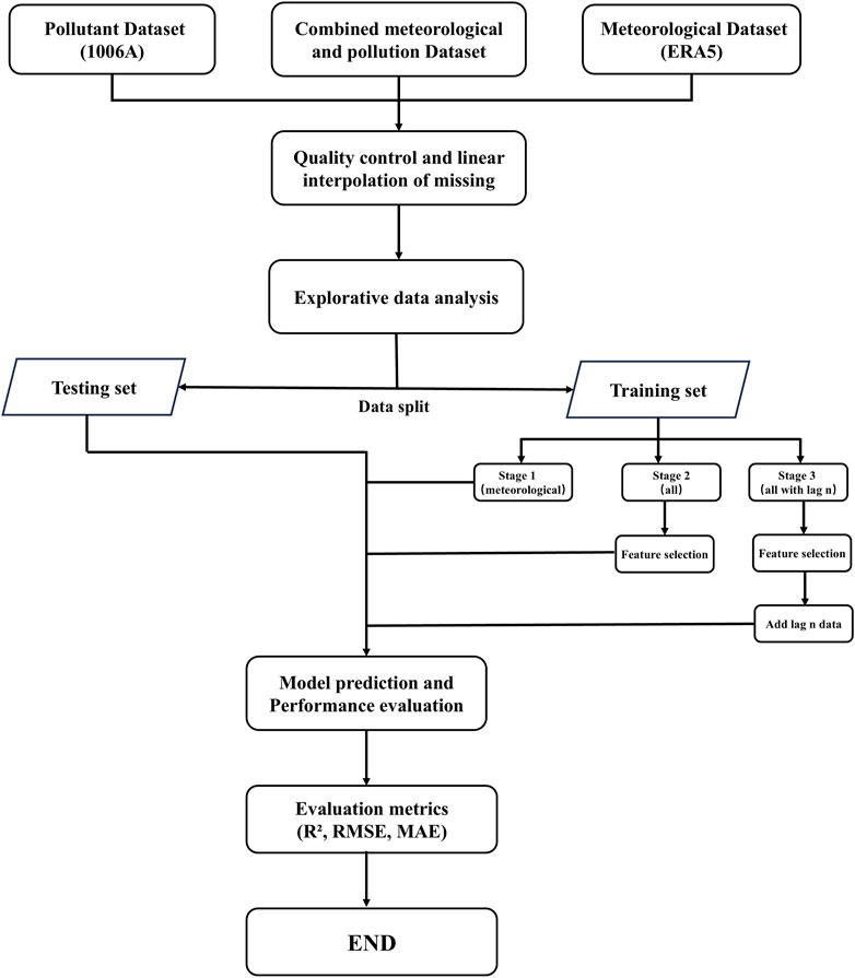
Figure 1. Data preprocessing and modeling process.

For predicting ozone concentration changes, this study selects three types of machine learning methods: 1. Traditional methods: KNN (based on distance similarity) and SVM (kernel space mapping); 2. Ensemble tree models: Random Forest, Decision Tree, XGBoost (feature splitting and gradient boosting); 3. Neural networks: MLP (fully connected networks), LSTM, and its variants (modeling temporal dependencies). These machine learning methods have multiple hyperparameters that can be adjusted to improve performance. The GridSearchCV function from the Python Sklearn library was used. This function employs the TimeSeriesSplit cross-validation method to evaluate each set of parameter combinations. Some hyperparameters were also manually adjusted and tested to verify whether they returned the highest accuracy score. Each machine learning model tested with hyperparameter tuning was trained using hourly data from 1 year (2023). We created an algorithm to try different parameter combinations and return the best parameters, fine-tuning sensitive model parameters (such as the hidden layer dimension of LSTM and the subtree depth of XGBoost) based on validation set performance to ensure the globally optimal parameter combination. To obtain the best parameter combination for each machine learning model during both experimental stages, different hyperparameter adjustments were made in each experiment process (see Tables 2, 3). The experimental parameters for adding lag features followed those used in the meteorological variables and pollutant variables experiments.

Table 2

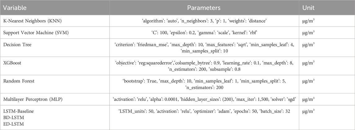
Table 2. Machine learning algorithm parameters for Python Scikit-Learn and Keras (meteorological variables prediction).

Table 3

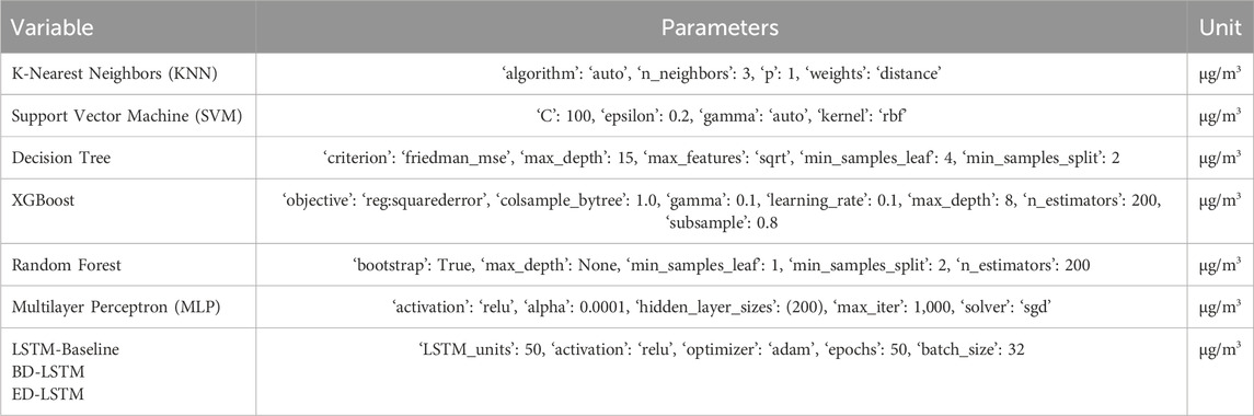
Table 3. Machine learning algorithm parameters for Python Scikit-Learn and Keras (meteorological and pollutant variables prediction).

Figure 2 shows the distribution of the collected data. It is evident that these data do not conform to a Gaussian distribution but instead exhibit some skewness or multimodal characteristics. This non-Gaussian distribution may be caused by various complex factors, such as fluctuations in meteorological conditions, uneven spatial distribution of pollution sources, and intermittent changes in industrial activities (Li, 2020a; Zhang et al., 2023). Understanding these distribution characteristics is helpful for model selection and performance optimization.

Figure 2

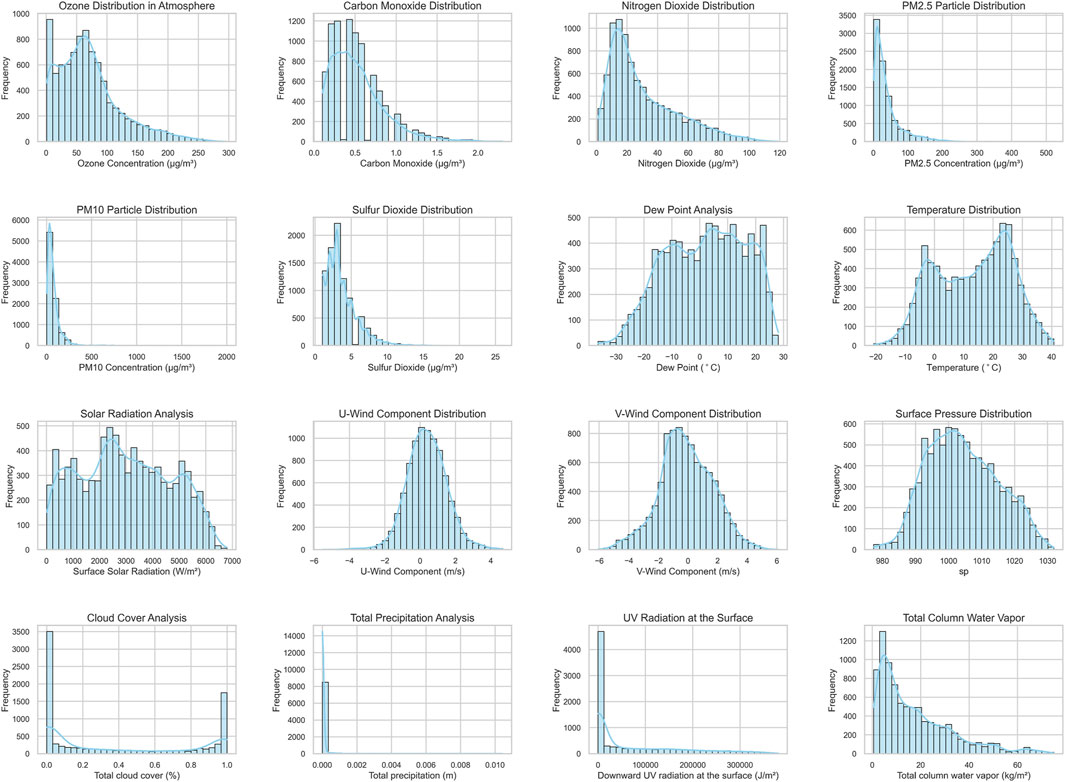
Figure 2. Distribution of pollutant and meteorological data.

2.2 Methodology

This section introduces the machine learning methods used in this study for ozone concentration prediction and the model evaluation metrics. The machine learning methods compared in this study include SVM, XGBoost, RF, MLP, KNN, Decision Tree, as well as Long Short-Term Memory (LSTM) and its variants, which are suitable for handling nonlinear problems. The evaluation metrics used include the coefficient of determination (R²), Root Mean Square Error (RMSE), and Mean Absolute Error (MAE).

The MLP (Multilayer Perceptron) (Wang and Lu, 2006), also known as Artificial Neural Network, consists of an input layer, an output layer, and several hidden layers. The input layer receives external inputs, while the hidden and output layers process the signals using activation functions, with the output layer providing the final results. By using the GridSearchCV function from the Python Sklearn library to tune the MLP, it was found that the relu function yielded the best results. Therefore, relu is used as the activation function in this study. The computation process for MLP is as follows:

$h_j={\displaystyle \sum _{i=0}^N}{W}_{ij}{x}_{ij}$

In the formula, $h_j$ represents the weighted sum of all inputs to the neuron node in the hidden layer, $W_{ij}$ denotes the weight from the input layer neuron to the hidden layer neuron, and $x_{ij}$ represents the input value.

$a_j=g\left(h_j\right)=g\left({\displaystyle \sum _{i=0}^N}{W}_{ij}{x}_{ij}\right)$

In the formula, $a_j$ represents the output value of the neuron in the hidden layer, g(x) is the activation function, and $a_j=x_{ij}$, meaning the output value of the neuron in the current layer is equal to the input value of the neuron in the next layer.

$y=g\left(h_k\right)=g\left({\displaystyle \sum _{i=0}^N}{W}_{jk}{x}_{jk}\right)$

In the formula, y represents the value of the output layer, i.e., the predicted value. $h_k$ is the weighted sum of all inputs to the neuron node in the output layer, and $W_{jk}$ denotes the weight from the hidden layer neuron to the output layer neuron.

Support Vector Regression (SVR) (Ortiz-García et al., 2010) maps the original low-dimensional input x into a high-dimensional feature space $\phi \left(x\right)$ using a nonlinear function $\phi$. In the high-dimensional space, it seeks a linear regression hyperplane to address nonlinear problems in the low-dimensional space. SVR is known for its resistance to overfitting and strong generalization capabilities. The linear function in the high-dimensional feature space can be expressed as:

$y=〈W_{\phi }\left(x\right)〉+b$

In the formula, y represents the output, $〈W_{\phi }\left(x\right)〉$ denotes the inner product in the feature space, where W is the weight vector, and b is the bias constant. These parameters W and b can be determined by minimizing the risk function as follows:

$Q=\frac{{‖w‖}^2}{2}+C{\displaystyle \sum _{i=1}^N}{L}_g\left(x_i,y_i,f\right)$

Where:

$L_g\left(x_i,y_i,f\right)=\left\{\begin{array}{l}\left|y_i-f\left(x_i\right)\right|-\epsilon ,\left|y_i-f\left(x_i\right)\right|\geqq \epsilon ,\\ 0,else\end{array}\right.$

In the formula: C: A pre-defined penalty coefficient that penalizes errors greater than ε epsilon. ε epsilon: The margin of tolerance, representing the deviation allowed between the predicted values and the actual observations in the training set. Errors within ε epsilon are not penalized.

The choice of the kernel function can significantly affect the model’s performance. Therefore, this study selected the radial basis function (rbf) kernel, which is well-suited for learning and effectively handles nonlinear data.

Compared to the SVR algorithm, the Random Forest (RF) model (Stafoggia et al., 2020) is an ensemble learning algorithm known for its simplicity, high accuracy, and strong generalization ability. It is also more robust to noise and outliers. The algorithm generates multiple sampling sets using random sampling techniques, trains multiple weak learners on these sets, and then combines their outputs through an aggregation strategy to produce the final model output. For regression tasks, a simple averaging method is typically used, where the regression results from all weak learners are averaged arithmetically to yield the final model output. The calculation process is as follows:

$m_{ni}=y_i-f_{n-1}\left(x_i\right)$

In the formula, $m_{ni}$ represents the residual, $y_i$ is the observed value of the $i$ sample, $f_{n-1}\left(x_i\right)$ is the predicted value from the previous learner, the residual is fitted to obtain a residual model $g_n\left(x\right)$, and the regression tree is updated accordingly:

$f_n\left(x\right)=f_{n-1}\left(x\right)-g_n\left(x\right)$

Decision Tree (Gao et al., 2021) is a tree-structured supervised learning method used for solving classification and regression problems. It recursively divides the data into subsets to construct a decision tree that maximizes information gain, ultimately achieving the prediction objective. Its core idea is to build branches based on features and use leaf nodes to represent the prediction results.

At each split, the decision tree attempts to find the optimal feature and split point within the given feature space to maximize the objective function (e.g., the increment of information gain or Gini index). Each resulting subset continues to recursively execute the same process until the stopping criteria are met (e.g., the node purity is sufficiently high or the number of samples falls below a predefined threshold). The prediction function in a decision tree can be expressed as:

$y=f\left(x\right)={\displaystyle \sum _{i=1}^M}{c}_i·I\left(x\in R_i\right)$

Where: y is the output value. M is the number of leaf nodes. $c_i$ is the predicted value in leaf node $R_i$ (category label for classification tasks or mean/median for regression tasks). $I\left(x\in R_i\right)$ is an indicator function that signifies whether the sample x falls within the region $R_i$.

The K-Nearest Neighbors Regression model (KNN Regression) (Zhang et al., 2022a) is an instance-based non-parametric supervised learning method that makes predictions by measuring the similarity (usually distance) between data points. In KNN regression, for a given input sample x, the model’s predicted output y is the weighted average of the target values of its k-nearest neighbors:

$\widehat{y}=\frac{1}{k}{\displaystyle \sum _{i\in N_k\left(x\right)}}{y}_i$

Where: $N_k\left(x\right)$ represents the index set of the k-nearest neighbors of sample x. $y_i$ is the target value of the i neighbor.

The core idea of Extreme Gradient Boosting (XGBoost) is to iteratively combine multiple weak learners (base models) into a strong learner using the gradient boosting algorithm (Zhang et al., 2022b) In each iteration, XGBoost constructs a new weak learner based on the gradient of the prediction error from the previous model and optimizes the loss function to improve prediction accuracy.

For a given dataset $\left(x_i,y_i\right)$, the model’s prediction output can be expressed as:

$\widehat{y_i}={\displaystyle \sum _{k=1}^K}{f}_k\left(x_i\right)$

Where: K is the total number of trees. $f_k$ represents the k weak learner, where $f_k\in F$. F denotes the set of all regression trees. XGBoost trains the model by minimizing the objective function:

$L={\displaystyle \sum _{i=1}^n}l\left(y_i,\widehat{y_i}\right)+{\displaystyle \sum _{k=1}^K}\mathrm{\Omega }\left(f_k\right)$

Where: $l\left(y_i,\widehat{y_i}\right)$ is the loss function (e.g., squared error or log loss). $\mathrm{\Omega }\left(f_k\right)=\mathrm{{\rm Y}}T+\frac{1}{2}\lambda {‖\omega ‖}^2$ represents the complexity of the model. $\mathrm{{\rm Y}}$ and $\lambda$ are regularization parameters.

LSTMs (Long Short-Term Memory Networks) fundamentally diverge from traditional machine learning algorithms in their temporal processing capabilities, demonstrating superior performance in time series modeling. We systematically evaluated three LSTM variants: Standard LSTM, Bidirectional LSTM (BD-LSTM), and Encoder-Decoder LSTM (ED-LSTM). As specialized recurrent neural networks (RNNs), these architectures overcome the gradient vanishing problem inherent in conventional RNNs through innovative memory cell designs with forget gates (Zhang et al., 2021). This mechanism enables selective retention or discarding of historical information from preceding timesteps, thereby effectively capturing long-range temporal dependencies critical for ozone prediction.

Notably, LSTMs have demonstrated strong empirical validity in air quality forecasting research, particularly in one-step-ahead prediction scenarios (Xayasouk et al., 2020). successfully implemented an LSTM integrated with deep autoencoders to predict particulate matter levels using historical weather variables (humidity, wind speed/direction, temperature) (Tiwari et al., 2021). further advanced multi-step forecasting through multivariate BD-LSTM configurations, establishing their predictive superiority. In our experimental framework, all three LSTM variants underwent rigorous performance benchmarking against six conventional machine learning algorithms across three experimental phases.

The metrics used in our evaluation are as follows: for evaluating the performance of the prediction models, this study uses the coefficient of determination (R²), root mean square error (RMSE) and mean absolute error (MAE). Each evaluation metric measures the model accuracy from different perspectives and effectively compares the prediction accuracy of different models. For RMSE and MAE, smaller values indicate better performance, while for R², larger values indicate better performance.

$R^2=1-\frac{{\sum }_{i=0}^{n-1}{\left(\widehat{y_i}-{\overline{y}}_i\right)}^2}{{\sum }_{i=0}^{n-1}{\left(y_i-{\overline{y}}_i\right)}^2}$

$RMSE\left(y,\widehat{y}\right)=\sqrt{\frac{1}{n}{\displaystyle \sum _{i=0}^{n-1}}{\left(y_i-\widehat{y_i}\right)}^2}$

$\text{MAE}\left(y,\widehat{y}\right)=\frac{1}{n}{\displaystyle \sum _{i=0}^{n-1}}{‖y_i-\widehat{y_i}‖}_1$

2.3 Feature variable selection

XGBoost is an ensemble learning algorithm based on Gradient Boosting Decision Trees (GBDT), capable of effectively handling large-scale data and providing built-in feature importance evaluation (Li, 2022). Feature importance is measured by calculating the gain (Gain) of each feature at the splitting nodes, reflecting the contribution of each feature to the improvement of model performance. SHAP is a game-theory-based model explanation method that quantifies the marginal contribution of each feature to the prediction outcome, offering both global and local model interpretability. The advantage of SHAP lies in its consistency and fairness, providing reliable explanations in complex models with multiple feature interactions (Wang et al., 2024). By combining XGBoost and SHAP, this section aims to identify the most influential feature variables for ozone concentration prediction, thereby improving the computational efficiency of the model.

We first evaluated the performance of XGBoost. XGBoost achieved an R² of 0.767, RMSE of 11.35, and MAE of 8.82 on the test set, indicating its good predictive capability. This provides a reliable basis for the subsequent feature variable importance analysis. The built-in feature importance evaluation of XGBoost showed that NO₂, SSR, UVB, and TCWV are key features influencing ozone concentration prediction (Figure 3). To further validate the reliability of the feature variable importance analysis, we used SHAP analysis to interpret XGBoost. The SHAP analysis results (Figure 4) were highly consistent with the XGBoost results, indicating that NO₂, SSR, UVB, and TCWV have a significant impact on predicting ozone concentration.

Figure 3

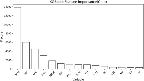
Figure 3. Feature importance in the XGBoost prediction model.

Figure 4

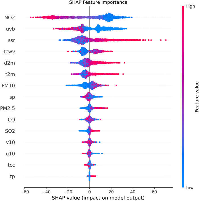
Figure 4. Feature selection based on SHAP importance.

Based on the feature variable importance analysis, we selected the top 11 important features to train the model. These variables represent a combination of pollutant and meteorological factors, which can balance prediction accuracy and computational complexity to some extent, providing a solid foundation for subsequent model optimization. After simplifying the input model parameters, the model’s performance was similar to that of the full model (RMSE decreased from 11.35 to 11.39, R² decreased from 0.767 to 0.766), but the computation time was reduced by 30%. This result indicates that feature variable selection helps improve computational efficiency and model interpretability while maintaining prediction performance.

3 Results

3.1 Ozone concentration prediction using meteorological variables

We used the hourly training dataset from 2023 to capture the variability and dynamics within the data. Since the data includes two main types of features: meteorological variables and pollutant variables, we designed a three-phase experimental process. In the first phase, only meteorological variables, such as UVB, SSR, D2M, and TCWV, were used to analyze the impact of these meteorological factors on ozone concentration. The second phase added the remaining pollutant variables, such as NO₂, PM₁₀, CO, and SO₂, based on the first phase. The third phase further introduced lag features for O₃ and NO₂ (lag-n) to capture dynamic characteristics within the time series.

After determining the best hyperparameters for each machine learning model using meteorological variables to create ozone prediction models via GridSearchCV in the Python Sklearn library, the data was split chronologically to avoid data leakage. The first 90% of the data was used as the training set, and the remaining 10% was used as the validation set for model evaluation. This approach ensures that the model predicts on entirely unseen data, allowing for a fair comparison and providing the final performance results.

In the first experiment, we only considered meteorological variables to predict ozone concentration, specifically: 2m dew point temperature, 2m temperature, surface net solar radiation, surface pressure, downward UV radiation at the surface, and total column water vapor. Importantly, this experiment aimed to assess the capability of machine learning in predicting ozone concentration based solely on meteorological variables. Table 4 presents the average performance of different machine learning methods in predicting ozone concentration using hourly meteorological data from the entire year of 2023. The metrics include R², root mean square error (RMSE), mean absolute error (MAE), and training time. The results show that for ozone concentration prediction using meteorological variables, LSTM models performed excellently in terms of accuracy and error control, especially ED-LSTM, which had the highest R² (0.479) across all models, along with the lowest RMSE (16.98 μg/m³) and MAE (13.77 μg/m³). This indicates that LSTM effectively captures complex dynamic features within the time series data and outperforms traditional machine learning models in prediction accuracy. In contrast, KNN and Decision Trees, despite having very short training times (0.01 and 0.02 s, respectively), performed poorly, with R² values of 0.215 and 0.192. XGBoost showed moderate performance (R² = 0.341) but did not reach the accuracy level of LSTM-based models. Overall, while LSTM models required longer training times, especially LSTM-Baseline and BD-LSTM (14.74 and 13.46 s, respectively), their accuracy advantages made them more stable for long-term predictions, capable of providing more precise ozone concentration predictions at higher time resolutions. Figure 5 compares the predicted and observed ozone concentrations from different models, clearly demonstrating the limitations of relying solely on meteorological variables for ozone prediction. Additionally, Figures 6, 7, showing R², RMSE, and MAE, further highlight the performance differences and emphasize the superior accuracy of LSTM-based models in predicting ozone concentration using meteorological variables.

Table 4

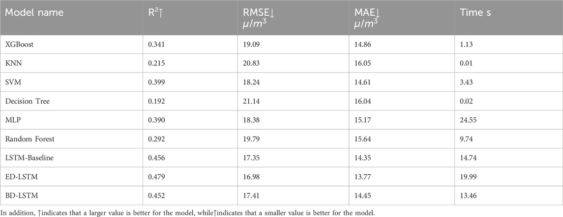
Table 4. Ozone prediction performance of each machine learning Model using meteorological variables.

Figure 5

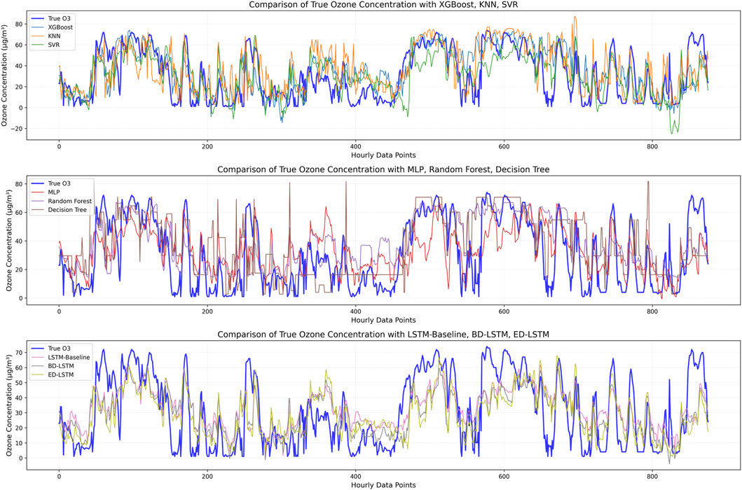
Figure 5. Comparison between observed O3 concentration and predicted O3 concentration when using meteorological variables for prediction.

Figure 6

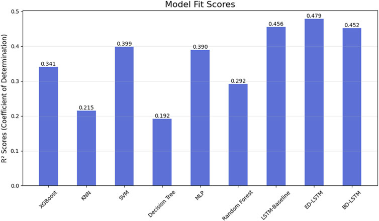
Figure 6. Fitting scores of predictions made by each model trained with meteorological variables: LSTM and its variants perform the best.

Figure 7

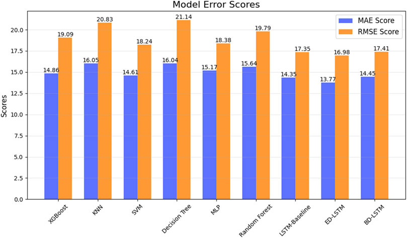
Figure 7. Similar to Figure 6, but showing the annual model error scores for MAE and RMSE. Both are in units of μg/m3.

In conclusion, when predicting ozone concentration using only meteorological variables, LSTM models, particularly ED-LSTM, perform the best. Although training times are longer, their accuracy advantage makes them the optimal choice. For scenarios requiring real-time, rapid predictions, traditional models like XGBoost may offer efficiency benefits, but their lower prediction accuracy limits their practical application. The next phase of experiments will integrate pollutant variables to improve model performance in more complex scenarios.

3.2 Ozone concentration prediction using meteorological and pollutant variables

In the first experiment, we used only meteorological variables as inputs and employed various machine learning models to predict ozone pollution. The main purpose of this phase was to evaluate the independent contribution of meteorological conditions to ozone concentration prediction. In the second experiment, to further improve prediction performance, we added pollutant variables (including CO, PM₁₀, PM_2.5, NO₂, and SO₂) to the meteorological variables. These pollutant variables, being major precursors or indirect influencers of ozone, significantly impact the generation and consumption processes of ozone (Wang et al., 2017). The best hyperparameters for each machine learning model using both meteorological and pollutant variables to create ozone prediction models were determined using the GridSearchCV function in the Python Sklearn library. By combining both meteorological and pollutant variables, we can capture the factors affecting ozone variations more comprehensively.

As can be seen from Table 5, it is clear that introducing pollutant variables significantly improved the performance of all models, especially XGBoost. When only meteorological variables were used, XGBoost had an R² of 0.341, which was quite modest. However, after introducing pollutant variables, XGBoost’s R² increased significantly to 0.767, RMSE decreased from 19.09 μg/m³ to 11.35 μg/m³, and MAE decreased from 14.86 μg/m³ to 8.82 μg/m³, demonstrating its strong prediction performance after incorporating pollutant variables. In addition, KNN, which performed excellently in terms of training time with only meteorological variables (training time of 0.01 s), had a low R² of 0.215 and poor prediction accuracy. After introducing pollutant variables, KNN’s performance improved, with an R² of 0.661, but it still lagged behind XGBoost. SVM and MLP performed weakly in the meteorological-only ozone prediction experiment, especially MLP, which had an R² of only 0.390, but the training time was as high as 24.55 s, revealing its efficiency bottleneck when handling large-scale data. After adding pollutant variables, both SVM and MLP saw improvements in their R² values, reaching 0.661 and 0.627, respectively, but their computational efficiency remained low, especially with MLP, where the training time increased to 29.18 s after including pollutant variables. Decision Trees performed poorly when predicting ozone using both meteorological and pollutant variables, with an R² of 0.685. Although the training time was the shortest (0.04 s), its prediction accuracy was lower than that of models like XGBoost. Random Forest showed stable performance in both experiments. After incorporating pollutant variables, its R² was 0.749, RMSE was 11.79 μg/m³, MAE was 9.25 μg/m³, and the training time was 3.13 s. While it did not outperform XGBoost, it still performed quite well. LSTM-based models also showed stable performance, but due to their longer training times, their computational efficiency was lower, and their R² values were not as high as those of XGBoost and Random Forest. Figure 8 compares the predicted and observed ozone concentrations of different machine learning models using both meteorological and pollutant variables. It clearly shows that predicting ozone concentration using both meteorological and pollutant variables is far more accurate than using meteorological variables alone.

Table 5

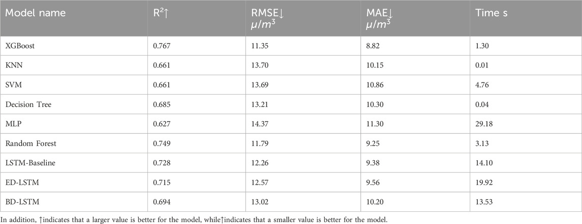
Table 5. Ozone prediction performance of each machine learning Model using meteorological and pollutant variables.

Figure 8

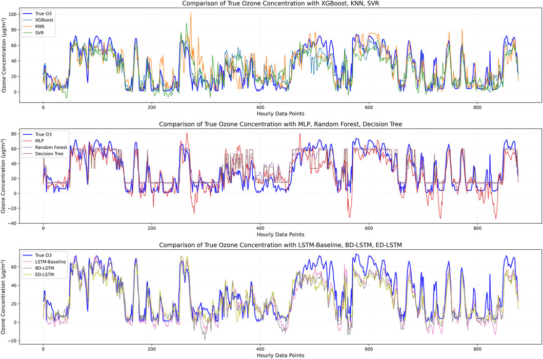
Figure 8. Comparison between observed O3 concentration and predicted O3 concentration when using meteorological and pollutant variables.

Overall, after incorporating pollutant variables, XGBoost is undoubtedly the best choice, as it achieves optimal accuracy and efficiency. KNN is suitable for scenarios requiring efficient predictions but has lower prediction accuracy. Other models, such as SVM, MLP, and LSTM, still have room for improvement in both computational efficiency and prediction accuracy.

3.3 Ozone prediction using lagged feature variables

In the previous two experiments, machine learning did not consider the information from lagged feature variables, which made it difficult to effectively capture the dynamics in the data. As slight bias still existed in the previous experiment, we attempted to reduce algorithmic bias by introducing lagged feature variables for O₃ and NO₂(O₃ and NO₂ concentrations at previous time points) to create a Lagged Feature Prediction Model (LFPM). O₃ and NO₂ time series data exhibit significant dynamic characteristics, as shown in the Autocorrelation Function (ACF) plot (Figure 9). The autocorrelation analysis reveals that O₃ exhibits significant time lag effects, with its autocorrelation remaining high over a longer lag range, indicating that past ozone concentrations have a significant impact on future concentration changes. Meanwhile, as a major precursor to O₃, changes in NO₂ concentration directly influence the generation and consumption processes of ozone.

Figure 9

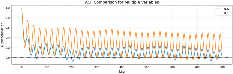
Figure 9. Autocorrelation of lagged feature time series data: Strong periodicity in the dataset.

The chemical formation process of O₃ involves key precursors such as NO₂ and generates O₃ through a series of complex photochemical reactions (Figure 10). In this process, NO₂ is decomposed by short-wave ultraviolet radiation into nitric oxide (NO) and atomic oxygen (O (³P)), and then the atomic oxygen reacts with oxygen molecules (O₂) and a third body (M) to form ozone (O₃) (Jian et al., 2022). Additionally, O₃ reacts with NO to form NO₂ and O₂, creating a dynamic equilibrium. Therefore, in order to better capture the interaction between O₃ and NO₂ in the time series and their contribution to the prediction, setting lagged feature variables for O₃ and NO₂ is crucial. These lagged feature variables can reflect the potential impact of ozone and nitrogen dioxide concentrations at previous time points on current and future concentration changes, thereby improving the model’s accuracy in predicting ozone concentrations.

Figure 10

Figure 10. Key chemical equations for Ground-Level Ozone formation and depletion (Highlighting substances relevant to this study) model.

Therefore, when predicting ozone concentration, simultaneously introducing lagged feature variables for O₃ and NO₂ to create the LFPM helps better capture the temporal information and dynamic relationships between the pollution variables, thus improving prediction accuracy. In this experiment, we considered lagged feature variables for O₃ and NO₂ in ozone concentration prediction. In brief, this section aims to investigate the impact of introducing lagged feature variables on the accuracy of ozone prediction.

To this end, we introduced lag features in predicting ozone concentration to account for the influence of historical O₃ and NO₂ data. In the first scenario (Lag 1), the input data includes 12 variables, including pollutants (CO, SO₂, PM₂.₅, PM₁₀), meteorological factors (d2m, t2m, ssr, sp, uvb, tcwv), as well as the lagged O₃ and NO₂ data from the previous hour (O₃.Lag1, NO₂.Lag1). In the second scenario (Lag 3), the input variables are expanded to 16, adding the lagged O₃ and NO₂ data from the second and third hours (O₃.Lag1, O₃.Lag2, O₃.Lag3, NO₂.Lag1, NO₂.Lag2, NO₂.Lag3). Additionally, to enhance the rigor of the experiment and effectively avoid data leakage caused by lag features, we set reasonable buffers for different lag lengths. In the Lag one scenario, a 1-h buffer was applied, while in the Lag three scenario, a 3-h buffer was used. This ensures complete independence between the training and testing data, thus enhancing the reliability and scientific integrity of the experimental results.

Table 6 defines the lagged feature variables for O₃ and NO₂ that were considered. Figures 11, 12 show the comparison between the observed values and predicted ozone values, while Tables 7 and 8 present the prediction accuracy. From the figures, we can visually observe that, as expected, considering the lagged feature variables for O₃ and NO₂ helps improve the prediction of the machine learning models (Figures 11, 12).

Table 6

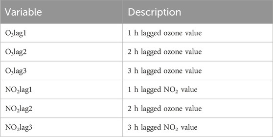
Table 6. Lagged feature variables for O₃ and NO₂.

Figure 11

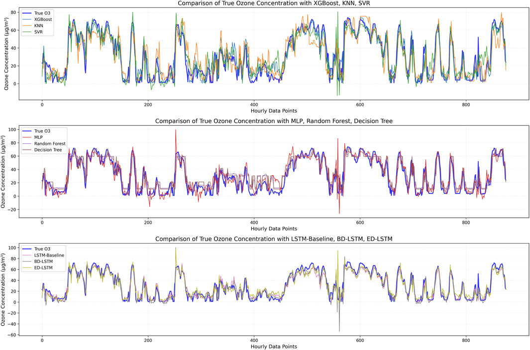
Figure 11. Comparison between observed O3 concentration and predicted O3 concentration, including lagged features of O3 (lag 1) and NO2 (lag 1).

Figure 12

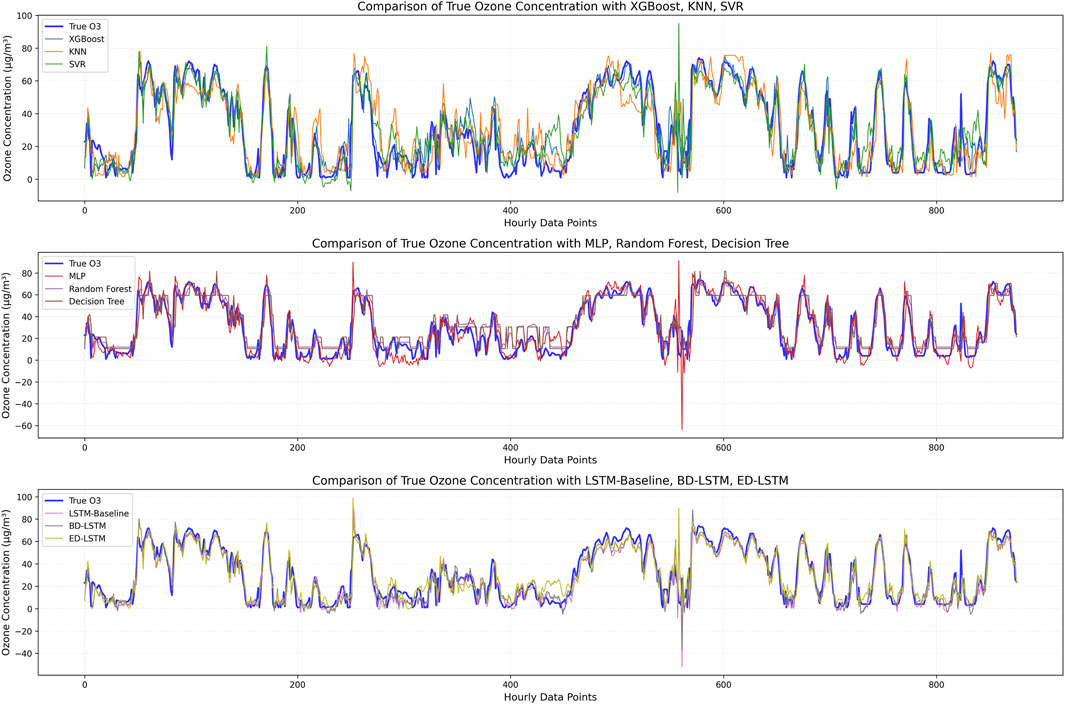
Figure 12. Comparison between observed O3 concentration and predicted O3 concentration, including lagged features of O3 (lag 3) and NO2 (lag 3).

Table 7

Table 7. Ozone prediction performance of each machine learning Model with Lag 1 O₃ and NO₂ lagged feature variables.

Table 8

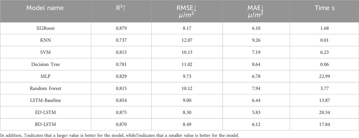
Table 8. Ozone prediction performance of each machine learning Model with Lag 3 O₃ and NO₂ lagged feature variables.

Tables 7 and 8 provide the prediction results and error levels using lagged feature variables for O₃ and NO₂ with lag one and lag 3, respectively. The results in Table 7 show that the XGBoost model achieved the best performance across all metrics, and importantly, the training time was only 1.37 s. In this case study, XGBoost is the optimal model, offering both high accuracy and efficiency. The XGBoost model achieved the highest R² value (0.879) and the lowest RMSE (8.17 μg/m³). Among the trained models, all models with the inclusion of lagged feature variables for O₃ and NO₂ were able to capture the ozone trend well, with reasonable prediction errors. Therefore, this result confirms that the lagged feature variables for O₃ and NO₂ (O₃.Lag1, O₃.Lag2, and O₃.Lag3; NO₂.Lag1, NO₂.Lag2, and NO₂.Lag3) are sufficient to enhance the prediction quality of the machine learning models studied.

The results in Table 8 indicate that when considering the inclusion of lagged feature variables for O₃ and NO₂ over three periods in the input for ozone prediction, the conclusions are consistent with those in Table 7. Specifically, XGBoost still outperforms other models in terms of both accuracy and efficiency. Additionally, by incorporating lagged feature variables for O₃ and NO₂ over three periods, the performance of most models becomes more stable. More precisely, all metrics show slight improvements, and the prediction error range in Figure 12 becomes noticeably narrower and more concentrated. Therefore, we can conclude that XGBoost is the best model in terms of accuracy and efficiency, and further confirm that introducing lagged feature variables for O₃ and NO₂ helps the model better capture the temporal information and dynamic relationships between pollutants, thereby improving prediction accuracy.

However, in long-term forecasting tasks, the prediction ability of each model shows a declining trend, with accuracy gradually decreasing as the forecast horizon increases (as shown in Figure 13). This may be related to the highly dynamic nature of ozone concentration and the attenuation effect of lag features in long-term forecasting. When the prediction window extends to 6 h or longer, the complex nonlinear relationships between pollutants and meteorological variables may lead to cumulative errors, making it difficult for the models to maintain high-accuracy predictions. Furthermore, as the prediction horizon increases, the influence of lag features, which are further from the current time, on future ozone concentration gradually weakens, further exacerbating prediction uncertainty. However, in short-term forecasting (e.g., predicting the next hour), after adding lag features, all models achieve relatively high prediction accuracy, indicating that lag information significantly improves short-term ozone concentration prediction.

Figure 13

Figure 13. Variation trends of R2 and RMSE for Each Model in 24-Hour Forecasting.

Ensuring that the selected best prediction model is statistically superior to other models is very important. One common method is to compare the performance of models through statistical tests, such as the Chow test and the Breusch-Pagan test (Demšar, 2006). In this study, we used the Diebold-Mariano test (Diebold and Mariano, 2002) to compare the prediction accuracy of each model. The Diebold-Mariano test is commonly used in economics and finance to evaluate the performance of different prediction models. The advantage of this test is that it does not require prediction errors to follow a specific distribution, making it a reliable statistical test for comparing the predictive capabilities of different models under the assumption of no bias. Additionally, the Diebold-Mariano test is easy to implement and its results are straightforward to interpret, making it a widely used tool for comparing prediction model performance.

The core idea of the Diebold-Mariano test is to evaluate the prediction accuracy by comparing the mean squared errors of the two models’ predictions. Specifically, the p-value generated by the test reflects whether there is a significant difference in the mean squared errors of the prediction errors between the two models. The null hypothesis assumes that there is no significant difference in prediction accuracy between the two models, while the alternative hypothesis suggests that one model outperforms the other in terms of prediction performance. To conduct this test, we first calculate the differences between the prediction errors of the two models, then assess the statistical significance of this difference using a t-test. If the p-value is less than the significance level, it indicates that one model is significantly superior to the other in terms of prediction performance.

Figure 14 shows the p-value matrix heatmap generated by the Diebold-Mariano test. The p-values range from 0 to 1, with values closer to 0 providing stronger evidence against the null hypothesis, indicating a significant difference in prediction performance between the two models. If the p-value is less than 0.05, it suggests that the null hypothesis can be rejected, and the conclusion can be made that there is a significant difference in prediction performance between the two models. The results in Figure 14 show that most p-values are close to 0, providing strong evidence to reject the null hypothesis, indicating that there is a significant difference in prediction performance between most of the model comparisons. However, there are some exceptions, such as combinations involving (SVM), (KNN), and (XGBoost), which have relatively higher p-values (0.05 or above), suggesting that the prediction performance differences between these models may not be significant.

Figure 14

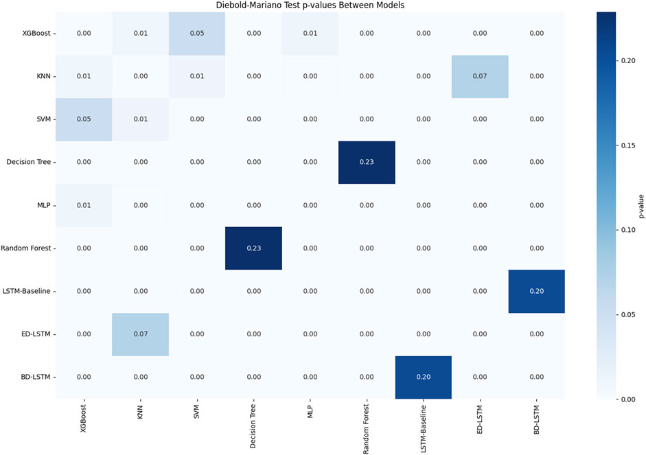
Figure 14. DM test of the models.

Overall, this indicates that the XGBoost model performs the best among all tested models, as both the Diebold-Mariano test and evaluation metrics (such as R², RMSE, and MAE) show it has the strongest prediction accuracy. The model’s R² value is 0.879, indicating a strong correlation between the predicted and actual ozone concentrations. Furthermore, the RMSE value is 8.17 μg/m³ and the MAE value is 6.10 μg/m³, suggesting that the average difference between the predicted and actual values is very small.

4 Discussion

This study systematically evaluates machine learning models for ground-level ozone prediction in Beijing, demonstrating the critical role of temporally-embedded feature engineering in enhancing forecasting accuracy. Our proposed Lagged Feature Prediction Model (LFPM), incorporating historical O₃ and NO₂ concentrations (t-1 to t-3 h), achieved superior performance across all evaluated algorithms. XGBoost emerged as the optimal predictor with LFPM integration (R² = 0.879, RMSE = 8.17 μg/m³, MAE = 6.10 μg/m³), outperforming conventional static models by 30% in R² improvement–a testament to its capability in resolving ozone’s spatiotemporal dynamics through gradient-boosted tree ensembles.

The temporal dependency analysis revealed significant predictive gains from lagged features, particularly highlighting the photochemical memory effect: historical NO₂ levels (as precursor) and O₃ auto-correlation collectively explain >40% of feature importance through SHAP decomposition. This aligns with ozone formation mechanisms requiring cumulative solar radiation exposure and precursor accumulation (Bais et al., 2015), suggesting LFPM effectively encodes critical photochemical timescales (typically 2–5 h in urban environments (Sadanaga et al., 2003)).

Comparative benchmarking against prior studies contextualizes our advancements:

• Nonlinear methods: Our XGBoost-LFPM (R² = 0.873) substantially exceeds reported neural network performances (R² = 0.49 (Sinha and Singh, 2021)) and RF benchmarks (R² = 0.72 (Shukla et al., 2021)).

• Model universality: The absence of a consistent “best algorithm” across studies (Capilla, 2016; Shukla et al., 2021; Sinha and Singh, 2021) underscores the necessity for case-specific model selection, particularly when adapting to regional emission profiles and monitoring network architectures.

While XGBoost demonstrated superior efficiency-accuracy tradeoffs, alternative models showed context-dependent merits.

• MLP captured complex meteorological-O₃ nonlinearities more effectively in reduced feature spaces, albeit with 3× longer training times.

• SVM exhibited greater stability under sparse data conditions, suggesting potential utility in sensor-limited deployments.

Notably, feature space optimization through SHAP-guided selection identified NO₂, surface solar radiation (ssr), uvb, and total column water vapor (tcwv) as photochemically critical variables. Retraining with the top 11 features maintained predictive fidelity (ΔR²<0.01) while reducing computational overhead by 30% – a crucial advancement for real-time air quality management systems requiring operational efficiency.

5 Conclusion

The detrimental impacts of elevated ground-level ozone (O₃) on urban atmospheric systems and public health underscore the critical need for precise ozone forecasting to inform environmental governance. As a canonical secondary pollutant, tropospheric O₃ production exhibits intricate dependence on synergistic interactions between meteorological drivers (temperature, atmospheric stability, solar irradiance) and precursor emissions (NO₂, CO, VOCs). While stratospheric ozone serves vital UV-protective functions, elevated tropospheric ozone concentrations demonstrate nonlinear coupling with photochemical regimes–where precursor reactivity modulates diurnal patterns and spatial heterogeneity under varying meteorological conditions. Current predictive frameworks struggle to resolve these spatiotemporally dynamic interactions, particularly in balancing model fidelity with operational efficiency across urban pollution hotspots.

This investigation systematically benchmarks nine machine learning architectures (XGBoost, LSTM variants, RF, etc.) for Beijing’s ozone prediction, establishing XGBoost-integrated LFPM (Lagged Feature Prediction Model) as the superior paradigm (R² = 0.879, RMSE = 8.17 μg/m³). Our methodology reveals two critical advancements:

1. Dual-input optimization combining real-time meteorology and multi-hour pollutant lag terms (t-1 to t-3) enhances predictive skill by 30% compared to single-modality inputs;

2. SHAP-guided feature selection identifies NO₂ and solar radiation parameters as photochemical linchpins, enabling 30% computational acceleration without accuracy loss.

These findings position machine learning–particularly gradient-boosted ensembles–as transformative tools for urban ozone management. Future work must address real-world deployment challenges: hybrid architectures integrating chemical transport models with adaptive ML, edge-computing optimizations for sensor networks, and explainable AI frameworks for policy translation. The ultimate objective remains developing city-specific digital twins that bridge predictive accuracy, operational efficiency, and regulatory actionability in combating ozone pollution.

Data availability statement

The original contributions presented in the study are included in the article/supplementary material, further inquiries can be directed to the corresponding authors.

Author contributions

ZtL: Conceptualization, Data curation, Formal Analysis, Investigation, Methodology, Project administration, Software, Validation, Visualization, Writing–original draft, Writing–review and editing. ZgL: Writing–review and editing, Conceptualization, Project administration, Formal Analysis. WZ: Formal Analysis, Funding acquisition, Project administration, Supervision, Writing–review and editing. JY: Funding acquisition, Project administration, Supervision, Writing–review and editing. ZC: Conceptualization, Formal Analysis, Writing–review and editing. TC: Conceptualization, Investigation, Writing–review and editing. SL: Data curation, Validation, Writing–review and editing. YX: Data curation, Visualization, Writing–review and editing. XZ: Data curation, Software, Writing–review and editing.

Funding

The author(s) declare that no financial support was received for the research and/or publication of this article.

Acknowledgments

The authors gratefully acknowledge the meteorological reanalysis data provided by the European Centre for Medium-Range Weather Forecasts (ECMWF) and the hourly pollutant observation data from the National Air Quality Monitoring Network of China.

Conflict of interest

The authors declare that the research was conducted in the absence of any commercial or financial relationships that could be construed as a potential conflict of interest.

Generative AI statement

The author(s) declare that no Generative AI was used in the creation of this manuscript.

Publisher’s note

All claims expressed in this article are solely those of the authors and do not necessarily represent those of their affiliated organizations, or those of the publisher, the editors and the reviewers. Any product that may be evaluated in this article, or claim that may be made by its manufacturer, is not guaranteed or endorsed by the publisher.

References

Bais, A. F., McKenzie, R. L., Bernhard, G., Aucamp, P. J., Ilyas, M., Madronich, S., et al. (2015). Ozone depletion and climate change: impacts on UV radiation. Photochem and Photobiological Sci. 14 (1), 19–52. doi:10.1039/c4pp90032d

PubMed Abstract | CrossRef Full Text | Google Scholar

Capilla, C. (2016). Prediction of hourly ozone concentrations with multiple regression and multilayer perceptron models. Int. J. SDP. 11, 558–565. doi:10.2495/sdp-v11-n4-558-565

CrossRef Full Text | Google Scholar

Chen, Z., Liu, R., Luo, Z., Xue, X., Wang, Y., and Zhao, Z. J. (2024). Prediction of autumn ozone concentration in the Pearl River Delta based on machine learning. Huan Jing ke Xue= Huanjing Kexue 45 (1), 1–7. doi:10.13227/j.hjkx.202302044

PubMed Abstract | CrossRef Full Text | Google Scholar

Cheng, M., Fang, F., Navon, I. M., Zheng, J., Tang, X., Zhu, J., et al. (2022). Spatio-temporal hourly and daily ozone forecasting in China using a hybrid machine learning model: autoencoder and generative adversarial networks. J. Adv. Model. Earth Syst. 14 (3), e2021MS002806. doi:10.1029/2021ms002806

CrossRef Full Text | Google Scholar

Comrie, A. C. (1997). Comparing neural networks and regression models for ozone forecasting. J. Air and Waste Manag. Assoc. 47 (6), 653–663. doi:10.1080/10473289.1997.10463925

CrossRef Full Text | Google Scholar

Demšar, J. (2006). Statistical comparisons of classifiers over multiple data sets. J. Mach. Learn. Res. 7, 1–30.

Google Scholar

Dhanya, G., Pranesha, T. S., Nagaraja, K., Chate, D. M., and Beig, G. (2022). Comprehensive modeling of seasonal variation of surface ozone over southern tropical city, Bengaluru, India. Nat. Environ. Pollut. Technol. 21 (3), 1269–1277. doi:10.46488/NEPT.2022.v21i03.033

CrossRef Full Text | Google Scholar

Diebold, F. X., and Mariano, R. S. (2002). Comparing predictive accuracy. J. Bus. and Econ. statistics 20 (1), 134–144. doi:10.1198/073500102753410444

CrossRef Full Text | Google Scholar

Du, J., Qiao, F., Lu, P., and Yu, L. (2022). Forecasting ground-level ozone concentration levels using machine learning. Resour. Conservation Recycl. 184, 106380. doi:10.1016/j.resconrec.2022.106380

CrossRef Full Text | Google Scholar

Ellingsen, K., Gauss, M., Van Dingenen, R., Dentener, F. J., Emberson, L., Fiore, A. M., et al. (2008). ‘Global ozone and air quality: a multi-model assessment of risks to human health and crops’. Build. Environ. 96, 101845. doi:10.5194/acpd-8-2163-2008

CrossRef Full Text | Google Scholar

Emberson, L. (2020). Effects of ozone on agriculture, forests and grasslands. Philosophical Trans. R. Soc. A Math. Phys. Eng. Sci. 378 (2183), 20190327. doi:10.1098/rsta.2019.0327

PubMed Abstract | CrossRef Full Text | Google Scholar

Gao, Y., Wang, Z., Zheng, T., and Peng, Z. R. (2021). Assessing neighborhood variations in ozone and PM2.5 concentrations using decision tree method. Build. Environ. 188, 107479. doi:10.1016/j.buildenv.2020.107479

CrossRef Full Text | Google Scholar

Jian, J., Hashemi, H., Wu, H., Jasper, A. W., and Glarborg, P. (2022). A reaction mechanism for ozone dissociation and reaction with hydrogen at elevated temperature. Fuel 322, 124138. doi:10.1016/j.fuel.2022.124138

CrossRef Full Text | Google Scholar

Li, J., Gao, Y., and Huang, X. (2020). The impact of urban agglomeration on ozone precursor conditions: a systematic investigation across global agglomerations utilizing multi-source geospatial datasets. Sci. Total Environ. 704, 135458. doi:10.1016/j.scitotenv.2019.135458

PubMed Abstract | CrossRef Full Text | Google Scholar

Li, K., Jacob, D. J., Liao, H., Zhu, J., Shah, V., Shen, L., et al. (2019). A two-pollutant strategy for improving ozone and particulate air quality in China. Nat. Geosci. 12 (11), 906–910. doi:10.1038/s41561-019-0464-x

CrossRef Full Text | Google Scholar

Li, K., Jacob, D. J., Shen, L., Lu, X., De Smedt, I., and Liao, H. (2020a). Increases in surface ozone pollution in China from 2013 to 2019: anthropogenic and meteorological influences. Atmos. Chem. Phys. 20 (19), 11423–11433. doi:10.5194/acp-20-11423-2020

CrossRef Full Text | Google Scholar

Li, Y. (2020b). Estimation of ground-level ozone concentration based on GBRT. China Environ. Sci. 40 (3), 997–1007.

Google Scholar

Li, Z. (2022). Extracting spatial effects from machine learning model using local interpretation method: an example of SHAP and XGBoost. Comput. Environ. Urban Syst. 96, 101845. doi:10.1016/j.compenvurbsys.2022.101845

CrossRef Full Text | Google Scholar

Ma, R., Ban, J., Wang, Q., Zhang, Y., Yang, Y., He, M. Z., et al. (2021). Random forest model based fine scale spatiotemporal O3 trends in the Beijing-Tianjin-Hebei region in China, 2010 to 2017. Environ. Pollut. 276, 116635. doi:10.1016/j.envpol.2021.116635

PubMed Abstract | CrossRef Full Text | Google Scholar

Maji, K. J., and Namdeo, A. (2021). Continuous increases of surface ozone and associated premature mortality growth in China during 2015–2019. Environ. Pollut. 269, 116183. doi:10.1016/j.envpol.2020.116183

PubMed Abstract | CrossRef Full Text | Google Scholar

Mallet, V., Stoltz, G., and Mauricette, B. (2009). Ozone ensemble forecast with machine learning algorithms. J. Geophys. Res. Atmos. 114 (D5), 2008JD009978. doi:10.1029/2008JD009978

CrossRef Full Text | Google Scholar

Monks, P. S., Archibald, A. T., Colette, A., Cooper, O., Coyle, M., Derwent, R., et al. (2015). Tropospheric ozone and its precursors from the urban to the global scale from air quality to short-lived climate forcer. Atmos. Chem. Phys. 15 (15), 8889–8973. doi:10.5194/acp-15-8889-2015

CrossRef Full Text | Google Scholar

Niu, Y., Chen, R., Kan, H., and Zhou, M. (2022). Regional effects unlikely to explain association between ozone and cardiovascular mortality in China - authors' reply, Lancet. Planet. Health, 6, e780, e781. doi:10.1016/S2542-5196(22)00224-8

PubMed Abstract | CrossRef Full Text | Google Scholar

Ortiz-García, E. G., Salcedo-Sanz, S., Pérez-Bellido, Á., Portilla-Figueras, J., and Prieto, L. (2010). Prediction of hourly O3 concentrations using support vector regression algorithms. Atmos. Environ. 44 (35), 4481–4488. doi:10.1016/j.atmosenv.2010.07.024

CrossRef Full Text | Google Scholar

Peng, J., Shang, B., Xu, Y., Feng, Z., and Calatayud, V. (2020). Effects of ozone on maize (Zea mays L.) photosynthetic physiology, biomass and yield components based on exposure- and flux-response relationships. Environ. Pollut. 256, 113466. doi:10.1016/j.envpol.2019.113466

PubMed Abstract | CrossRef Full Text | Google Scholar

Sadanaga, Y., Matsumoto, J., and Kajii, Y. (2003). Photochemical reactions in the urban air: recent understandings of radical chemistry. J. Photochem. Photobiol. C Photochem. Rev. 4 (1), 85–104. doi:10.1016/S1389-5567(03)00006-6

CrossRef Full Text | Google Scholar

Shukla, K., Dadheech, N., Kumar, P., and Khare, M. (2021). Regression-based flexible models for photochemical air pollutants in the national capital territory of megacity Delhi. Chemosphere 272, 129611. doi:10.1016/j.chemosphere.2021.129611

PubMed Abstract | CrossRef Full Text | Google Scholar

Sinha, A., and Singh, S. (2021). ‘Dynamic forecasting of air pollution in Delhi zone using machine learning algorithm’, 2, pp. 40–53.

Google Scholar

Stafoggia, M., Johansson, C., Glantz, P., Renzi, M., Shtein, A., de Hoogh, K., et al. (2020). A random forest approach to estimate daily particulate matter, nitrogen dioxide, and ozone at fine spatial resolution in Sweden. Atmosphere 11 (3), 239. doi:10.3390/atmos11030239

CrossRef Full Text | Google Scholar

Suciu, L. G., Griffin, R. J., and Masiello, C. A. (2017). Regional background O₃ and NO_x in the Houston–Galveston–Brazoria (TX) region: a decadal-scale perspective. Atmos. Chem. Phys. 17, 6565–6581. doi:10.5194/acp-17-6565-2017

CrossRef Full Text | Google Scholar

Sun, H., Fung, J. C., Chen, Y., Chen, W., Li, Z., Huang, Y., et al. (2021). Improvement of PM2.5 and O3 forecasting by integration of 3D numerical simulation with deep learning techniques. Sustain. Cities Soc. 75, 103372. doi:10.1016/j.scs.2021.103372

CrossRef Full Text | Google Scholar

Tan, X., Qian, Y., Wang, H., Fu, J., and Wu, J. (2022). Analysis of the spatial and temporal patterns of ground-level ozone concentrations in the guangdong–Hong Kong–Macao greater bay area and the contribution of influencing factors. Remote Sens. 14 (22), 5796. doi:10.3390/rs14225796

CrossRef Full Text | Google Scholar

Tiwari, A., Gupta, R., and Chandra, R. (2021). Delhi air quality prediction using LSTM deep learning models with a focus on COVID-19 lockdown. arXiv Prepr. arXiv.

Google Scholar

Wang, D., and Lu, W.-Z. (2006). Ground-level ozone prediction using multilayer perceptron trained with an innovative hybrid approach. Ecol. Model. 198 (3), 332–340. doi:10.1016/j.ecolmodel.2006.05.031

CrossRef Full Text | Google Scholar

Wang, H., Liang, Q., Hancock, J. T., and Khoshgoftaar, T. M. (2024). Feature selection strategies: a comparative analysis of SHAP-value and importance-based methods. J. Big Data 11 (1), 44. doi:10.1186/s40537-024-00905-w

CrossRef Full Text | Google Scholar

Wang, J., Dong, J., Guo, J., Cai, P., Li, R., Zhang, X., et al. (2023). Understanding temporal patterns and determinants of ground-level ozone. Atmos. (Basel). 14, 604. doi:10.3390/atmos14030604

CrossRef Full Text | Google Scholar

Wang, N., Lyu, X., Deng, X., Huang, X., Jiang, F., and Ding, A. (2019). Aggravating O3 pollution due to NOx emission control in eastern China. Sci. Total Environ. 677, 732–744. doi:10.1016/j.scitotenv.2019.04.388

PubMed Abstract | CrossRef Full Text | Google Scholar

Wang, T., Xue, L., Brimblecombe, P., Lam, Y. F., Li, L., and Zhang, L. (2017). Ozone pollution in China: a review of concentrations, meteorological influences, chemical precursors, and effects. Sci. Total Environ. 575, 1582–1596. doi:10.1016/j.scitotenv.2016.10.081

PubMed Abstract | CrossRef Full Text | Google Scholar

Xayasouk, T., Lee, H., and Lee, G. (2020). Air pollution prediction using long short-term memory (LSTM) and deep autoencoder (DAE) models. Sustainability 12 (6), 2570. doi:10.3390/su12062570

CrossRef Full Text | Google Scholar

Yang, J., and Zhao, Y. (2023). Performance and application of air quality models on ozone simulation in China – a review. Atmos. Environ. 293, 119446. doi:10.1016/j.atmosenv.2022.119446

CrossRef Full Text | Google Scholar

Yang, X.-T., Kang, P., Wang, A. Y., Zang, Z. L., and Liu, L. (2024). Prediction of ozone pollution in Sichuan Basin based on random forest model. Huan Jing ke Xue= Huanjing Kexue 45 (5), 2507–2515. doi:10.13227/j.hjkx.202304226

PubMed Abstract | CrossRef Full Text | Google Scholar

Zhang, B., Song, C., and Jiang, X. (2022a). Spatiotemporal prediction of O3 concentration based on the KNN-Prophet-LSTM model. Heliyon 8 (11), e11670. doi:10.1016/j.heliyon.2022.e11670

PubMed Abstract | CrossRef Full Text | Google Scholar

Zhang, B., Zhang, Y., and Jiang, X. (2022b). Feature selection for global tropospheric ozone prediction based on the BO-XGBoost-RFE algorithm. Sci. Rep. 12 (1), 9244. doi:10.1038/s41598-022-13498-2

PubMed Abstract | CrossRef Full Text | Google Scholar

Zhang, L., Wang, L., Tang, G., Xin, J., Li, M., Li, X., et al. (2023). Comprehensively exploring the characteristics and meteorological causes of ozone pollution events in Beijing during 2013–2020. Atmos. Res. 294, 106978. doi:10.1016/j.atmosres.2023.106978

CrossRef Full Text | Google Scholar

Zhang, X., Zhang, Y., Lu, X., Bai, L., Chen, L., Tao, J., et al. (2021). Estimation of lower-stratosphere-to-troposphere ozone profile using long short-term memory (LSTM). Remote Sens. 13 (7), 1374. doi:10.3390/rs13071374

CrossRef Full Text | Google Scholar

Zheng, X., Orellano, P., Lin, H. l., Jiang, M., and Guan, W. j. (2021). Short-term exposure to ozone, nitrogen dioxide, and sulphur dioxide and emergency department visits and hospital admissions due to asthma: a systematic review and meta-analysis. Environ. Int. 150, 106435. doi:10.1016/j.envint.2021.106435

PubMed Abstract | CrossRef Full Text | Google Scholar

Zhou, Z., Qiu, C., and Zhang, Y. (2023). A comparative analysis of linear regression, neural networks and random forest regression for predicting air ozone employing soft sensor models. Sci. Rep. 13 (1), 22420. doi:10.1038/s41598-023-49899-0

PubMed Abstract | CrossRef Full Text | Google Scholar

Zhu, W., Li, Y., Jiang, H., Zhang, X., Huang, Y., and Wang, P. (2024). Regionally differentiated responses of chlorophyll-a concentrations to reduced human activity during COVID-19 lockdown in the San Francisco bay area. J. Environ. Manage. 373, 123801. doi:10.1016/j.jenvman.2024.123801

PubMed Abstract | CrossRef Full Text | Google Scholar