Uncertainty analysis of field trials of low-cost Bi-TiO2-P25 solar photocatalyst for sustainable water treatment

Solar photocatalysis has the potential to reduce chemical and microbial contaminants in water and make it safer for consumption in an effective and sustainable manner. This has been studied and proven well under laboratory-scale conditions. In our previous work, the developed solar photocatalyst, Bi-${\text{TiO}}_2$-P25 has been tested for its efficiency in reducing total coliform from natural waters under solar light. Along with the promising results (up to 99% reduction of total coliform and 99.9% reduction of Escherichia coli in 2 hours), the uncertainties due to environmental factors associated with the process were also observed. The reaction rate was largely impacted by the change in sunlight intensity over the treatment or different initial concentrations of contaminants in natural water. Therefore, it becomes essential to understand how the performance would be impacted in such varied conditions to predict the optimum results. This paper discusses how the treatment time could be impacted by uncertainties affecting either the kinetic rate constant, or the initial concentration of bacteria, or both, as well as external factors such as solar intensity and other randomly varying factors during the treatment. Mathematically exact results are derived and future development trends, and challenges are discussed while providing a prospective outlook for the deployment of solar photocatalysis at pilot scale.

1 Introduction

Surface water bodies are valuable resources of water supply but highly prone to chemical and microbial contamination (Walker et al., 2019; Singh et al., 2024; Syeed et al., 2023). Chemical contamination is primarily caused by untreated industrial wastewater being discharged into water bodies, introducing pollutants such as dyes, antibiotics, pesticides, and more. Microbial contamination, on the other hand, is mainly the result of both natural processes and anthropogenic activities. Once contaminated, the microbial level can rise rapidly by bacteria multiplication and chemical contamination can lead to several resistances such as antibiotic resistance, algal blooms, etc. (Stevenson et al., 2015). The most common microorganisms that can be present in surface waters are total coliforms, fecal coliforms, and E. coli (E. coli) due to either the organisms found in water or animals having access to that surface water body (Cabral, 2010). Effective and sustainable treatment of surface water can not only utilize that resource but also lead to healthy and safe water consumption throughout the world. For such treatments, chlorination has been proven an effective approach for decades but it has its own limitations; for example, it ends up creating harmful by-products in water which are toxic to consume (Al-Abri et al., 2019). To overcome that, Advanced Oxidation Processes (AOPs) have gained attention in treating water in a more sustainable manner as they can mineralize the contaminants and avoid transferring them into solid and/or air phases (Hübner et al., 2024; Dhamorikar et al., 2024). Among AOPs, photocatalytic oxidation, in particular, is acknowledged to be highly effective in degrading both chemical as well as microbial contaminants in water treatment (Kuspanov et al., 2024; Serik et al., 2024). In order to make this technique even more sustainable, efforts are being put on to drive this technology using solar light (Ren et al., 2021).

Previous field studies (Porley et al., 2020) and assessment of catalyst substrates (Porley and Robertson, 2020) strongly indicate the possibilities of using this technology in a sustainable manner in real-world conditions. In a recent paper, a solar photocatalyst, Bi-${\text{TiO}}_2$-P25, was developed and tested for its ability to degrade chemical and microbial contaminants from water under laboratory-scaled conditions (Arora et al., 2025). Moreover, the developed photocatalyst offers the added benefit of being low-cost, as it is made from affordable materials, e.g., ${\text{TiO}}_2$ which is one of the most stable, versatile and studied photocatalyst (Alimard et al., 2024). The estimated raw material cost is approximately 5 USD/g, with 1 g of catalyst coating approximately 150 g of treating substrate (i.e., glass chips). Considering that 150 g of chips can treat up to 15 L of water, the total treatment amounts to 0.33 USD/L.

To assess the efficiency of catalyst to degrade chemical organic contaminant and (E. coli) in laboratory scale tests, 4-Chlorophenol was chosen to study microbial degradation (Arora et al., 2025). On achieving efficient results, the study was scaled up, and field trials were conducted in rural India in March’23, where the photocatalyst was tested to degrade total coliform and E. coli in real-world water in the presence of sunlight (Arora et al., 2025). However, field tests have primarily focussed on microbial contaminant degradation to adress the specific need of the area.The results unveiled that the developed catalyst can reduce up to 99% of total coliform and 99.9% of E. coli in 2 h under direct sunlight. However, the treatment process was notably influenced by independent variables, including solar light intensity, bacterial contamination levels, and the reusability of the photocatalyst. After achieving such promising results in field trials, it becomes crucial to understand how environmental uncertainties can affect solar photocatalytic oxidation and how the technology can be improved to achieve even better performances. Advancements in this direction will allow the transfer of technology to a practical scale. For example, the statistics of the treatment time as a function of uncertainties affecting the process variables will allow to better quantify the probability of failure given the size of the reactor and the catalyst or, vice-versa, design the best reactor size and catalyst by imposing the level of risk, etc.

In the present work, two types of uncertainties affecting the reaction process are considered. The first one is the statistical variability of the reaction parameters, namely, the reaction constant and the initial concentration of bacteria. The so-called derived distribution approach is used to study how the statistical change in one or both parameters - considered belonging to a given statistical distribution - impacts the statistical distribution of the treatment time. The second one is the source of variability directly affecting the reaction dynamics via a continuously (randomly) changing reaction constant. The latter case corresponds to environmental noise effects influencing the reaction process such as variable cloudiness and radiation or imperfect and inhomogeneous mixing, which technically transform the reaction kinetics into a stochastic differential equation of the Langevin type (Cox and Miller, 1977; Gardiner et al., 1985; Van Kampen, 1992). Furthermore, the theory of stochastic processes is used to derive mathematically exact solutions for both the probability density functions of the concentration at all times and the treatment time.

2 Methodology

2.1 Bi-${\text{TiO}}_2$-P25 photocatalytic oxidation

The main steps of the low-cost methodology adopting Bi-${\text{TiO}}_2$-P25 as the photocatalyst in the laboratory as well as the field are shown in Figure 1. The process begins with synthesizing the solar photocatalyst and coating it on recycled glass chips. A more detailed description of the synthesis procedure, as well as the material characterization, is mentioned in the Supplementary Material. For laboratory analysis, the glass chips were immersed in the water to be treated and illuminated with light (UV led) of optimum wavelengths ($\lambda =365nm$ and $\lambda$ = 410 nm). Direct sunlight was also tested, as a reference case (Arora et al., 2025). In the field, transparent plastic bottles were used as containers for treatment. The bottles were filled with water to be treated and 45 g of catalyst-coated chips were added. The bottles were exposed to sunlight for 2 h and rotated every 15 min to ensure a uniform mixing of water during treatment (Arora et al., 2025).

Figure 1

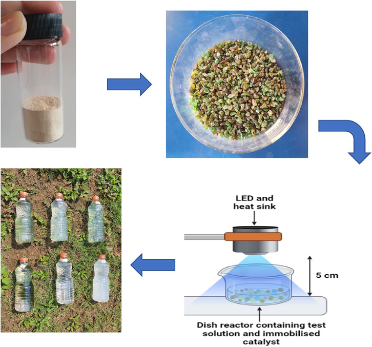
Figure 1. Illustration of the developed low-cost Bi-${\text{TiO}}_2$-P25 solar photocatalyst, the coating on the recycled glass chips followed by the laboratory, and the field test set up (modified from Arora et al., 2025).

For both laboratory experiments and field tests, it is well known that photocatalytic oxidation for microbial contaminants follows first-order kinetics (Lebedev et al., 2018; Tran et al., 2023; Masoom et al., 2024). Accordingly, the corresponding equation describing the temporal evolution of the concentration for the microbial contaminant, $A$, is:

$\left[A\left(t\right)\right]=\left[A\left(0\right)\right]e^{-Kt},(1)$

where $[A(t)]$ is the concentration of bacteria at time $t$, $[A(0)]$ is the initial concentration (i.e., at time $t=0$), and $K$ is the first-order rate constant. For the sake of brevity, the notation $[A(t)]$ is hereafter replaced by $c(t)$. Assuming a value $C_T$ as a target concentration to be reached at the end of the treatment, the treatment time, $\tau$, can be calculated as

$\tau =\frac{1}{K}\log \left[\frac{C_0}{C_T}\right](2)$

with $C_0$ the initial concentration of the microbial contaminant (i.e., $C_0=[A(0)]$).

2.2 Sources of indeterminate (random) errors

According to Equations 1 and 2, the reaction and the treatment time depend on the concentration of one reactant only. However, in practical situations the reaction is affected by many factors such as light intensity, catalyst pore size, solubility, catalyst efficiency, band gap, light distance, type of contaminant, etc. (Kim et al., 2024). The field studies also uncovered similar observations for instance, the rate and reaction efficiency significantly depended on environmental factors such as solar intensity and rotation frequency due to mass transport effects (Arora et al., 2025). Therefore, besides considering statistical changes in the initial concentration, it is important to take into account the sources of variability in the reaction constant to predict the photocatalyst’s and overall treatment’s efficiency. Two cases are studied in detail, namely,: i) uncertainty in the initial concentration for a given rate constant $K$, and ii) uncertainty in the rate constant for a given initial concentration, $C_0$, of the contaminant.

The uncertainty in the initial microbial concentration in the water (colony-forming unit (CFU) per mL) with which the treatment begins is given by the pollution process due to environmental or anthropic origin. As such, the concentration may have temporal and spatial variability (e.g., location of the water source). Without describing the current reason for such variability in the field measurements, in this work, simple probability density functions to describe the uncertainty in the initial concentration are accounted for.

The uncertainty in the reaction rate may depend on the environmental variables governing the treatment process, such as solar intensity, photocatalyst usage, and lifespan (i.e., the time after which regeneration is required). The latter effect, however, would affect the process at much larger timescales and is therefore not considered in this work. In a previous publication, Arora et al. (2025) showed that the treatment efficiency depends on the light wavelength used during the process, as well. Similarly to the previous case, an analysis based on the probability distribution functions is performed to study the effects induced by variability in the rate constant. Additionally, a stochastic approach considering a continuously changing constant rate is involved (see Section 2.4).

Additional sources of uncertainty in the final treatment time (Equation 2) are related to the variability of the target concentration, $C_T$, and the volume of treated water. In this regard, all the experimental and field measurements were performed using the same amount of water. Therefore, hereafter any uncertainty related to possible variation of treatment efficiency in relation to the treated volume is not considered. Noteworthy, the quantity $C_T$ this quantity usually represents the minimum concentration of bacteria considered safe to consume for a drinking water treatment technology. The value of $C_T$ may come from local or worldwide guidelines. For instance, the World Health Organisation (WHO) recommends that no coliform (in terms of CFU) must be present per 100 mL of water to match the drinking water standard (World Health Organization, 2022). Given that the value represents a target value based on different references, it is not correct to consider it as a random variate for the same treatment. Accordingly, it is considered deterministic and set equal to an exemplary value $C_T=50$ CFU/mL throughout the analysis.

2.3 Derived distribution approach

The derived distribution approach (Kottegoda and Rosso, 2008) allows calculating the probability distribution function (pdf) of a variable, $y=f(x)$, where $x$ is a random variable with known pdf (i.e., $p_x(x)$) and $f(x)$ is a monotonic and derivable function on a certain interval $[X_1,X_2]$. Consequently, the variable $y$ is bounded within the interval $[f(x_1),f(x_2)]$. The rule of mass conservation for the pdf.s allows to write

$\left|{\int }_{f\left(X_1\right)}^{f\left(X_2\right)}{p}_y\left(y\right)dy\right|={\int }_{X_1}^{X_2}{p}_x\left(x\right)dx=1,(3)$

where the presence of the absolute value on the left-hand side term allows for neglecting the sign of the integral when $f(X_1)<f(X_2)$. Accordingly, $p_y(y)$ can be obtained from $p_x(x)$ by introducing the change of variable $x=f^{-1}(y)$ and by recalculating the increment $dx=|\frac{1}{f^{\prime }(x)}|dy$, i.e.,

$\left|{\int }_{f\left(X_1\right)}^{f\left(X_2\right)}{p}_y\left(y\right)dy\right|={\int }_{f\left(X_1\right)}^{f\left(X_2\right)}{p}_x\left(f^{-1}\left(y\right)\right)\left|\frac{1}{f^{\prime }\left(x\right)}\right|dy=1.(4)$

By comparing the two integrand functions and rearranging the terms it follows that

$p_y\left(y\right)=p_x\left(f^{-1}\left(y\right)\right)\left|\frac{dx}{dy}\right|=\frac{p_x\left(f^{-1}\left(y\right)\right)}{\left|\frac{dy}{dx}\right|},(5)$

where the term $\left|\frac{dy}{dx}\right|=|f^{\prime }(x)|$ is the first derivative of the function $f(x)$ and represents the Jacobian of the change of variable. Mathematically, this acts as a scaling factor between one coordinate set and another, thus ensuring that both statistical distributions represent actual density functions (i.e., have unit area).

The effect of concurrent variation of both the initial concentration $C_0$ and the rate constant $K$ can be obtained by interpreting the derived distribution - e.g., with respect to $K$ - as conditional to the choice of the other variate, i.e., $C_0$. Then, the following superstatistics leads to the pdf of the treatment times, $\tau$, including both variates

$p_{\tau }\left(\tau \right)={\int }_{\mathrm{\Omega }}{p}_{\tau }\left(\tau |c_0\right)p_{c_0}\left(c_0\right)d{c}_0,(6)$

where $p_{\tau }(\tau |c_0)$ is the derived distribution of the treatment times given the $p_k(k)$ as per Equation 5 and $p_{c_0}(c_0)$ is the pdf of the initial concentration. To notice, $\tau$, $c_0$, and $k$ are related by the deterministic first-order relationship (Equation (1)), which produces a distortion of the integration domain $\mathrm{\Omega }$, and may result in an integral over multiple regions (an example of the distorted domain is reported in Section 3.1, and in Figure 4A).

2.4 Stochastic kinetic reaction

Random temporal changes in the rate constant may affect the actual treatment time. By considering the possibility that $K$ may vary as a consequence of random fluctuations during the process, the notation $k(t)$ is put in place, and the first-order reaction equation becomes

$\frac{dc\left(t\right)}{dt}=-k\left(t\right)c\left(t\right),(7)$

subject to the initial condition that $c(0)=C_0$ and that the minimal concentration $c(\tau )=C_T$ is reached at the reaction time, $\tau$. It is of interest to consider $k(t)$ being affected by random fluctuations induced by factors affecting the treatment process (e.g., solar intensity, Section 2.2). As previously discussed, this can be the case originating from environmental noise caused by variable cloudiness and non-homogeneous mixing within the reactor. Accordingly, $k(t)=K-{\mathrm{\Delta }}_k(t)$ is considered, where ${\mathrm{\Delta }}_k(t)$ represents the displacement (noise) of $k(t)$ from the mean value $⟨k(t)⟩=K$. The noise term, ${\mathrm{\Delta }}_k(t)$, is taken from a Gaussian distribution with zero mean (i.e., ${\bar{\mathrm{\Delta }}}_k(t)=0$) and variance ${\sigma }_k^2=⟨{\mathrm{\Delta }}_k{(t)}^2⟩$. Consequently, one can write ${\mathrm{\Delta }}_k(t)=g(C(t))\xi (t)$ where $\xi (t)$ is a Gaussian uncorrelated (i.e., white) noise with zero mean and strength $g(c(t))$. Equation 7 can now be rewritten as

$\frac{dc\left(t\right)}{dt}=-Kc\left(t\right)+g\left(c\left(t\right)\right)c\left(t\right)\xi \left(t\right),(8)$

or, equivalently,

$dc\left(t\right)=-Kc\left(t\right)dt+g\left(c\left(t\right)\right)c\left(t\right)dW(9)$

where $dW=\xi (t)dt$ represents the Wiener process (Van Kampen, 1992).

Equations 8 and 9 represent the evolution equation of a stochastic process continuous in time and space (i.e., concentration) and affected by multiplicative white Gaussian noise (i.e., the noise term $\xi (t)$ is multiplied by the state variable $c(t)$). In this work, the attention is paid to the case of additive noise, that is when the noise term $\xi (t)$ is not multiplied by the variable concentration $c(t)$From a dynamic point of view, the noise term represents continuous corrections to the reaction trajectory independent of the concentration. Equation 8 can now be simplified by considering the particular case of $g(c(t))=\sigma /c(t)$, thus yielding

$\frac{dc\left(t\right)}{dt}=-Kc\left(t\right)+\sigma \xi \left(t\right),(10)$

where $\sigma$ is the process variance (Daly and Porporato, 2006). It can be shown that $\sigma$ and ${\sigma }_k(t)$ are related by the following relationship

$\sigma ={\sigma }_k\left(t\right)\sqrt{\frac{C{\left(t\right)}^2-{\sigma }_c{\left(t\right)}^2}{t}},(11)$

where $C(t)$ and ${\sigma }_c^2(t)$ are the mean concentration and its variance, respectively, at each time $t$.

Equation 10 is commonly referred to as the Ornstein-Uhlenbeck stochastic process (Uhlenbeck and Ornstein, 1930; Van Kampen, 1992). An example of numerically generated trajectories for this process (Equation 10) is given in Figure 2, from which clearly appears the statistical nature of the concentration and the time to reach the minimum concentration even when starting from the same initial concentration $C_0$.

Figure 2

Figure 2. Sample realizations of stochastic trajectories driving the process from the initial concentration $C_0$ to the minimum concentration, $C_T$. The reaction constant, $K$, and the variance of the process, $\sigma$, refer to the average trajectory drawn in black (deterministic trajectory). The corresponding pdf for the process, $p_c(c,t=3\text{h})$, and the arrival time, $p_{\tau }(t)$, are drawn in red and blue, respectively. (A) process with $\sigma =1\left[\frac{\mathrm{C}\mathrm{F}\mathrm{U}}{\mathrm{m}\mathrm{L}{\mathrm{h}}^{0.5}}\right]$; (B) process with $\sigma =4\left[\frac{\mathrm{C}\mathrm{F}\mathrm{U}}{\mathrm{m}\mathrm{L}{\mathrm{h}}^{0.5}}\right]$.

Solving Equation 10 cannot be done with usual methods given the stochastic nature of the process and therefore the loose mathematical meaning of the solution $c(t)$. However, a statistical mechanics approach allows for writing the balance equation for the evolution of the probability density function, $p_c(c,t)$, for the concentration, $c$ of the contaminant $A$ at all times, $t$. The balance equation is known as Chapman-Kolmogorov forward equation and reads

$\frac{\partial p_c\left(c,t\right)}{\partial t}=K\frac{\partial }{\partial c}c{p}_c\left(c,t\right)+D\frac{{\partial }^2}{\partial c^2}{p}_c\left(c,t\right),+\text{\hspace{0.17em}I.C\hspace{0.17em}and\hspace{0.17em}B.Cs.}(12)$

where $D={\sigma }^2/2$. The solution of Equation 12 requires one initial condition and two boundary conditions. As an initial condition, it is imposed that all trajectories start from the initial concentration at time $t=0$, i.e., $p_c(c,0)=\delta (c-C_0)$, with $\delta (\cdot )$ being the Dirac delta distribution. Boundary conditions are taken as $p_c(C_T,t)=0$ and $p_c(\infty ,t)=0$, where $c=C_T$ represents the lower boundary at the minimal concentration at which the treatment stops.

The exact solution for $p_c(c,t)$ reads (Daly and Porporato, 2006)

$p_c\left(c,t\right)=\sqrt{\frac{K}{2\pi D\left(1-e^{-2Kt}\right)}}{e}^{-\frac{K}{2D}\frac{{\left(c-C_0{e}^{-Kt}\right)}^2}{1-e^{-2Kt}}}.(13)$

From $p_c(c,t)$, it is of interest to find the distribution, $p_{\tau }(\tau )$, of the times $\tau$ to reach the lower boundary at $c=C_T$. This can be obtained via the so-called survivor function method, which requires to calculate

$p_{\tau }\left(\tau \right)=-\frac{d}{d\tau }{\int }_{C_T}^{\infty }{p}_c\left(c,\tau \right)dc.(14)$

After some algebra one obtains

$p_{\tau }\left(\tau \right)=\frac{C_0{e}^{K\tau }-C_T}{\sqrt{2\pi D}}{\left(\frac{K}{e^{2K\tau }-1}\right)}^{3/2}{e}^{K\tau -\frac{K}{2D}\frac{{\left(C_0-e^{K\tau }{C}_T\right)}^2}{e^{2K\tau }-1}}.(15)$

2.5 Numerical simulations

Numerical simulations for testing the derived distribution approach are performed via a standard MonteCarlo technique and the MatLab software (MatLab 2023b). In particular, random generation of either initial concentration $c_0$ or rate constant $k$ is performed by extracting 1000 values from three different probability distribution functions (i.e., uniform, log-normal, and Gaussian). The initial concentration, $c_0$, ranges from $C_1$ = 100 CFU/mL and $C_2$ = 700 CFU/mL, and the rate constant, $k$, varies between $K_1$ = 0.3 ${\text{h}}^{-1}$ and $K_2$ = 0.7 ${\text{h}}^{-1}$, which are consistent with the field measurements (Arora et al., 2025). The generated values are then accounted for to calculate the corresponding treatment time, $\tau$, using Equation 2. The generated distribution of treatment time, $p_{\tau }(\tau )$, is then graphically compared to the theoretical distribution calculated using the derived distribution approach (Equation 5).

As far as the stochastic model is concerned, the effects of changing the parameters of the distribution of $k(t)$, i.e., the mean value, $K$, and the process variance, $\sigma$, are investigated. The analysis is performed by calculating the main statistics of the treatment time pdf, $p_{\tau }(\tau )$ (Equation 15), that is the mean treatment time, $T={\int }_0^{\infty }t{p}_{\tau }(t)dt$, and the time variance, ${\sigma }_{\tau }={\int }_0^{\infty }{t}^2{p}_{\tau }(t)dt$.

3 Results and discussions

3.1 Derived distribution of process variates

In this study, three probability distributions are used to study the statistics of the water treatment method: uniform (Supplementary Equation S1), lognormal (Supplementary Equation S4), and normal (Supplementary Equation S7) distribution. Except for the uniform one, which is mainly used as a didactical case here, these statistical distributions are chosen because of their broad applicability in describing environmental process uncertainties (Kottegoda and Rosso, 2008). All the three distributions are scaled between minimum and maximum values based on experimental and field measurements (Arora et al., 2025), so that the condition ${\int }_{X_1}^{X_2}{p}_x(x)/P_{x}dx=1$ holds, where the scaling factor $P_x$ is given by the relationship $P_x={\int }_{X_1}^{X_2}{p}_x(x)dx$. The mathematical relationships of the pdf.s, $p_x(x)$, analyzed in this work, alongside the derived distribution of the treatment time, $p_{\tau }(\tau )$, are reported in the Supplementary Material (Supplementary Table S1).

Values for either $c_0$ or $k$ were numerically generated as i.i.d process from the uniform (Supplementary Equation S1), lognormal (Supplementary Equation S4), and normal (Gaussian, Supplementary Equation S7) distribution functions, respectively. For each generated value, the time $\tau$ required to reach $C_T$ was calculated by using the first order rate Equation 2 and the resulting empirical histogram of values compared with the corresponding theoretical distribution functions obtained via the derived distribution approach (Equation 5). For all the tested cases, the results are shown in Figure 3.

Figure 3

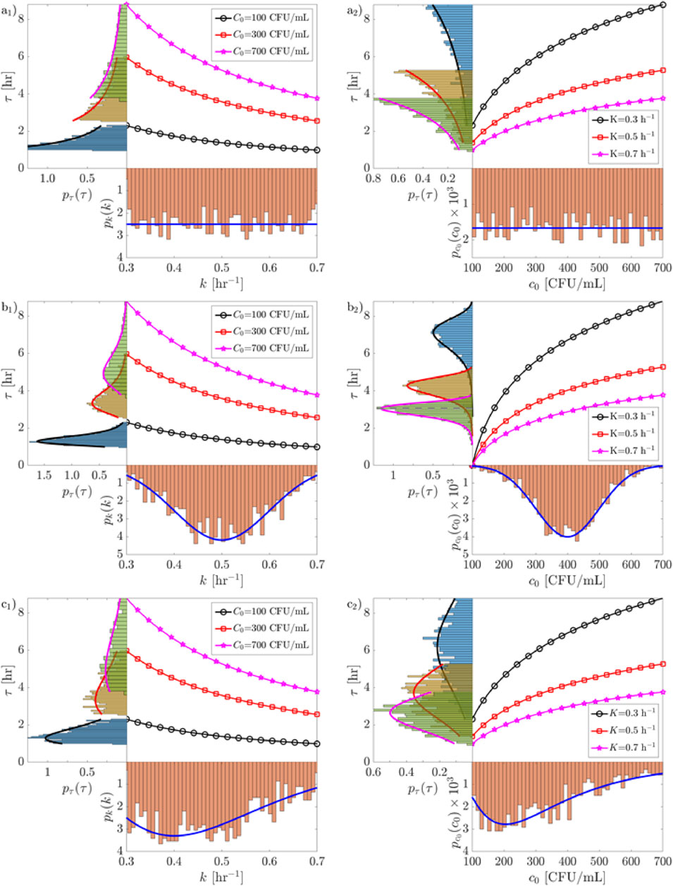
Figure 3. The probability distribution function, $p_{\tau }(\tau )$, of the treatment time, $\tau$, as a result of the derived distribution approach (Equation 5) for all the tested distributions of the rate constant, $k$, and the initial concentration, $c_0$. (a₁) uniform distribution of the constant rate, $k$ (Supplementary Equation S2) and $p_{\tau }(\tau )$ given by Supplementary Equation S2; (a₂) uniform distribution of the initial concentration, $c_0$ (Supplementary Equation S3) and $p_{\tau }(\tau )$ given by Supplementary Equation S3; (b₁) normal distribution of the constant rate, $k$ (Supplementary Equation S8) and $p_{\tau }(\tau )$ given by Supplementary Equation S8; (b₂) normal distribution of the initial concentration, $c_0$ (Supplementary Equation S9) and $p_{\tau }(\tau )$ given by Supplementary Equation S9; (c₁) log-normal distribution of the constant rate, $k$ (Supplementary Equation S5) and $p_{\tau }(\tau )$ given by Supplementary Equation S5; (c₂) log-normal distribution of the initial concentration, $c_0$ (Supplementary Equation S6) and $p_{\tau }(\tau )$ given by Supplementary Equation S6.

Consider first the case of the uniform distribution (Figure 3A): from a mathematical point of view, one sees that the reaction dynamics (exponential) transforms a uniform distribution into exponential ones (see Supplementary Table S1). Moreover, the effect of the reaction is that of introducing a skewness in the distribution of the treatment times, $\tau$. Regardless of the distribution affecting $c_0$ or $k$, the effect would be to deform such distributions by either introducing or modifying the original skewness and kurtosis values. In general, one expects the skew effect be positive as far as the uncertainty on $k$ is concerned. Conversely, the effect on the skewness is negative for that affecting the initial concentration, $c_0$. Figures 3B, C show that together with the asymmetry described by the skewness, the mode of the derived distribution may shift its position quite remarkably as a function of the other control parameter (i.e., with $c_0$ or $k$). This is rather important to consider for upscaling the treatment to the pilot scale, given that for skew distributions the mean and the mode of the distributions do not coincide anymore.

In order to move from the laboratory scale to the pilot scale, understanding the impact of all uncertainties involved in the process is critical. These uncertainties play a crucial role in optimizing the efficiency of water treatment using photocatalytic oxidation. In this regard, the proposed approach (i.e., the derived distribution, Equation 5) can be used to assess how uncertainties in $c_0$ and $k$ propagate to the treatment time required to reach the safer limit of contaminant concentration by using solar photocatalytic oxidation. For example, in the discussed case, it can be seen that the treatment time ranges between 1 and 8 h, i.e., in the best case scenarios (with high solar intensity, less polluted water, etc.) this treatment can make water safe to consume in around an hour and in worst cases it can take as long as 8 h. Therefore, in view of its large-scale application, this suggests introducing controls that restrict the variability of both the initial concentration $c_0$ and the reaction rate $k$ to narrow ranges.

The role of the initial concentration deserves some more attention, though. When the initial concentration of pollutants increases, the treatment time generally increases as well. This is because a higher concentration of contaminants requires more time for the photocatalyst to degrade them effectively. However, at higher concentrations, saturation effects or inhibition due to excess pollutant concentration might also reduce the overall efficiency of the process, thereby altering the expected degradation rate (Hanafi and Sapawe, 2020; Mangrulkar et al., 2012).

The variability in rate constant primarily depends on two factors: i) the life span of the photocatalyst and, ii) solar intensity during the treatment. Uncertainties arising from environmental noises (such as a change in solar intensities during treatment) or the photocatalyst’s life could lead to variation in the reaction rate constant, $k$. A higher $k$ means the reaction occurs more quickly, leading to a reduced treatment time. Conversely, a lower $k$ would result in longer treatment times, as the rate of degradation slows down. Variations in $k$ could arise from factors such as photocatalyst activity, light intensity, or environmental conditions (e.g., cloud cover, precipitation) that affect the reaction rate. The comprehensive understanding of the system’s dynamics is crucial for predicting and managing performance variations under real-world conditions, which often differ significantly from controlled experimental settings. Such insights enable the fine-tuning of operational parameters such as catalyst load, light intensity, and flow rates, thus improving sustained treatment efficiency and scalability. Ultimately, the proposed framework not only enhances the robustness of the technology but also facilitates its deployment in different environmental contexts, ensuring that the system remains effective even as operating conditions fluctuate.

As the final point of our analysis, an example of the resulting derived distribution of the treatment time in the case where both $c_0$ and $k$ vary following a uniform distributionis provided. This requires the approach shown in Equation 6 and the calculation of the integral therein. Figure 4A shows that the original rectangular domain, $[K_1,K_2],[C_1,C_2]$, becomes a figure with curved sides in the space $K,\tau$ and three integration domains $[\{{\tau }_1,{\tau }_2\},\{{\tau }_2,{\tau }_3\},\{{\tau }_3,{\tau }_4\}]$ (highlighted by different shading colors), the sum of which defines the whole domain of integration, $\mathrm{\Omega }$, of Equation 6. The result in this case is analytic and exact

$p_{\tau }\left(\tau \right)=\left\{\begin{array}{cc}\frac{C_1\left(1-\log \left[\frac{C_1}{C_T}\right]\right)+C_T{e}^{K_2\tau }\left(K_2\tau -1\right)}{\left(C_2-C_1\right)\left(K_2-K_1\right){\tau }^2}\hfill & {\tau }_1\le \tau \le {\tau }_2\hfill \\ \hfill \\ C_T\frac{e^{K_2\tau }\left(K_2\tau -1\right)-e^{K_1\tau }\left(K_1\tau -1\right)}{\left(C_2-C_1\right)\left(K_2-K_1\right){\tau }^2}\hfill & {\tau }_2<\tau \le {\tau }_3\hfill \\ \hfill \\ \frac{C_2\left(\log \left[\frac{C_2}{C_T}\right]-1\right)-C_T{e}^{K_1\tau }\left(K_1\tau -1\right)}{\left(C_2-C_1\right)\left(K_2-K_1\right){\tau }^2}\hfill & {\tau }_3<\tau \le {\tau }_4\hfill \\ \hfill \\ 0\hfill & \mathrm{o}\mathrm{t}\mathrm{h}\mathrm{e}\mathrm{r}\mathrm{w}\mathrm{i}\mathrm{s}\mathrm{e}\hfill \end{array}\right.(16)$

Figure 4

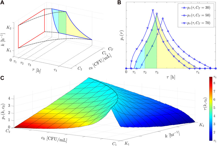
Figure 4. The bivariate derived distribution approach (Equation 6) and its application to calculate $p_{\tau }(\tau )$ in the case of uniform pdf.s for both $k$ and $c_0$. (A) The initial (red rectangular) and transformed domains of integration, $\mathrm{\Omega }$, showing the three sub-domains; (B) The $p_{\tau }(\tau ,C_T)$ at varying the final treatment concentration, $C_T$; (C) The surface plot of the bivariate pdf of the treatment time, $p_{\tau }(k,c_0)$. Shading colors represent the corresponding treatment time, $\tau$.

with ${\tau }_1=\frac{1}{K_2}\log \left[\frac{C_1}{C_T}\right]$, ${\tau }_2=\frac{1}{K_2}\log \left[\frac{C_2}{C_T}\right]$, ${\tau }_3=\frac{1}{K_1}\log \left[\frac{C_1}{C_T}\right]$, and ${\tau }_4=\frac{1}{K_1}\log \left[\frac{C_2}{C_T}\right]$. The corresponding pdf is shown in Figure 4B for three different final treatment concentrations, $C_T$, with the shaded regions of the curve $p_{\tau }(\tau ,C_T=50)$ corresponding to the three integration domains shown in Figure 4A. Figure 4C shows the bivariate joint distribution $p_{\tau }(k,c_0)$ obtained by re-substituting Equation 2 into Equation 16.

To summarize, the proposed study aims to highlight how treatment times are influenced by variations in initial concentration, $c_0$, or the rate constant, $k$, i.e., two key parameters in photocatalytic processes. On the contrary, this approach is not able to see how environmental noise forcing the reaction rate to change during the treatment would affect the treatment time. This is discussed in the next section.

3.2 Stochastic reaction dynamics

Examples of probability density functions $p_c(c,t)$ for the concentration at different times are shown in Figure 5A for different times. Notice, the initial peak distribution coincides with the Dirac delta function at the initial concentration $C_0$ at time $t=0$. As time evolves, uncertainty due to noise produces diverging trajectories and so the pdf increases its variance while losing mass when trajectories arrive at the boundary and the process stops. Increasing the intensity of the noise produces a higher variance for $p_c(c,t)$.

Figure 5

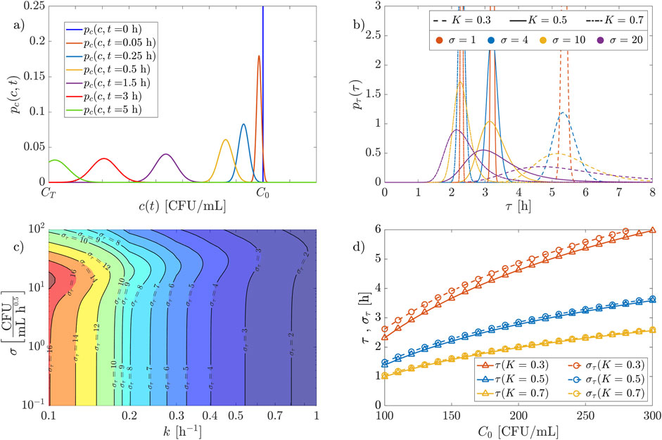
Figure 5. Probability distribution functions of concentration and treatment time for the Ornstein-Uhlenbeck process under analysis. (A) pdf of the concentration at different times ($K=0.3$, $\sigma =10$); (B) pdf of the treatment time, $p_{\tau }(\tau )$, for different combinations of the mean rate constant, $K$, and process variance, $\sigma$; (C) shaded plot of the treatment time variance, ${\sigma }_{\tau }$, as a function of the reaction constant and the process variance; (D) the mean treatment time, $T$, and its variance, ${\sigma }_{\tau }$, as a function of the initial concentration, $C_0$, for different values of the mean rate constant, $K$.

Although the solution for $p_c(c,t)$ is inspiring, for practical reasons, it is more interesting to focus on the statistics of the first passage time across the boundary, which corresponds to the treatment time, $\tau$ (Van Kampen, 1992; Daly and Porporato, 2006; Calvani and Perona, 2023). This time is also stochastic in nature and its statistical distribution, $p_{\tau }(t)$, is given by Equation 15, whose mean coincides with that of the deterministic dynamics, i.e., Equation 2. Examples of such pdf.s are shown in Figure 5B for the different mean rate constant $K$ and process noise intensity $\sigma$. The standard deviation of the distribution $p_{\tau }$, that is ${\sigma }_{\tau }$ is obtained numerically for a range of rate constants and noise intensities (Figure 5C) and a given initial concentration $C_0$. Notice that, as the environmental noise, $\sigma$, decreases in intensity, the variance of the treatment time, ${\sigma }_{\tau }$ depends on the mean rate constant $K$, only. Similarly, the effect of different initial concentrations is shown in Figure 5D. In this case, the change in ${\sigma }_{\tau }$ induced by small variations in the initial concentration, $C_0$, can be assessed by calculating the derivative $\partial {\sigma }_{\tau }/\partial C_0$. This procedure (i.e., sensitivity analysis) can be performed for any variable and parameters affecting the behavior of another variable. For the specific case shown in Figure 5D and regarding the treatment time variance, ${\sigma }_{\tau }$, the closed-form relationship of ${\sigma }_{\tau }$ appears to be quite cumbersome and, as such, a proper sensitivity analysis can only be performed via numerical tools. However, a quick insight into the sensitivity analysis can be graphically assessed in Figure 5C (for variation of $k$) and Figure 5D (for variation of $C_0$).

As the last aspect of our analysis, the level of dynamic environmental noise that may have affected the experimental data is assessed. From the experimental data, Arora et al. (2025) evaluated the rate constant of the reaction using a simple regression line to fit the experimental data on a logarithmic plot and obtain the mean rate constant, $K$. By taking the mean deviation of the experimental data from the theoretical reaction law, a first approximation of the standard deviation ${\sigma }_k$ that may have affected the rate constant of the reaction during the experiment is obtained. Using Equation 11, the strength of the noise $\sigma$ is calculated. From the mean concentration $C(t)$ and its measured standard deviation ${\sigma }_C(t)$ the regions within which the reaction was expected to evolve for all treatments are drawn. Such curves are shown in Figure 6 together with the experimental points, and some exemplary “noisy” trajectories for different treatments corresponding to different light sources. All clearly stay within the estimated range of variability (colored zone) predicted by the stochastic model. The same figure also shows the pdf.s of the concentration, $p_c(c,t)$ at the time $t=3h$ as well as the corresponding pdf.s of the treatment time, $p_{\tau }(t)$. Notice how the variance of the distribution for the sunlight treatment is higher with respect to that of the treatment with a light source of constant wavelength (e.g., $\lambda =410nm$, orange points and curves in Figure 6), which resulted in the highest mean rate constant.

Figure 6

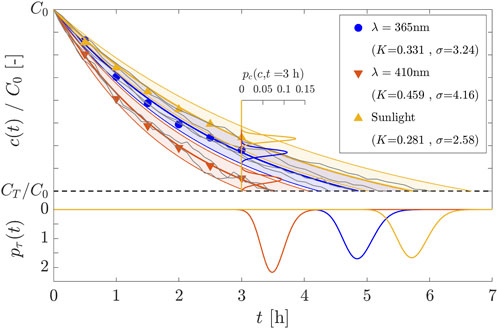
Figure 6. Experimental measurements (points), time evolution and associated pdf.s of the solar photocatalyst reaction using different light sources, i.e., wavelengths (blue for $\lambda$ = 365 nm, orange for $\lambda$ = 410 nm, yellow for direct sunlight). Data are plotted against the theoretical first-order reaction with $k=K$ (thick lines) and the shaded areas represent the corresponding regions of $k=K\pm {\sigma }_k$. Gray lines show some stochastic trajectories for each light source. The corresponding $p_c(c,t)$ and $p_{\tau }(t)$ are drawn.

In the present analysis, the process noise (rate constant variability) is considered to be originated by (random) variations in solar radiation and/or cloud cover, including the presence of precipitation. Due to the chemical nature, it is taken for granted that fluctuations in water temperature and pH affect the overall reaction dynamics. Furthermore, additional factors may impact the reaction dynamics, particularly for pilot-scale treatments. In this case, the size, shape, and orientation of the tank to sunlight can induce variations in concentration, potentially dampened by mechanical mixing. Determining the single contribution of each factor to the overall dynamic randomness is quite challenging, yet beyond the scope of this work. Nevertheless, the process noise $\sigma$ in Equation 10 may represent the presence of all the potential randomness sources. As such, one may proceed by calibrating its value based on available experimental or field data.

4 Conclusion

Following the field trials of the low-cost Bi-${\text{TiO}}_2$-P25 solar photocatalyst conducted in March 2023 in rural India, it was observed that the catalyst’s efficiency was significantly impacted by several external factors. Key variables such as the initial concentration of bacteria in the water and the solar intensity during treatment, which indirectly affected the reaction rate, played a major role in the process. This study explores the impact of these uncertainties on solar photocatalytic water treatment and the statistics of the treatment times. To model these uncertainties, in case they result from a pure field source basis, the derived distribution approach was employed, generating randomly distributed values (uniform, lognormal, and Gaussian) for the initial contaminant concentration, $C_0$, and the rate constant, $k$. Treatment times were then calculated for each set of values, and their histogram was validated against the theoretical distribution. This model offers a means to estimate average treatment times while accounting for uncertainties, provided that the distribution of the initial bacterial concentration and that of the rate constant are known and do not change during the treatment. The case of randomly varying rate constant was treated as environmental noise causing stochastic reaction dynamics, which was solved exactly as far as the pdfs of the concentration and the treatment times are concerned. This second approach is more meaningful to describe field-scale applications, i.e., where sunlight conditions (and so the rate constant) are not constant but potentially varying because of random cloudiness and other type of disturbances.

The two proposed approaches can be very useful in estimating treatment times during the process, enhancing the practicality of this technology in real-world applications. Additionally, they provide insights into the operational challenges posed by varying conditions and helps to optimize the design of solar photocatalytic systems. An extension of this study could involve examining the stochastic nature of water arrival, both in terms of volume and timing, and using this information to optimize the development of large-scale photocatalytic water treatment systems. This would be particularly valuable for designing photocatalytic reservoirs that can handle fluctuating water inputs and optimize treatment times for large-scale applications.

Data availability statement

The data analyzed in this study is subject to the following licenses/restrictions: The manuscript with the dataset is currently under review. See the reference in the submitted manuscript. Requests to access these datasets should be directed to YS5hcm9yYS00QHNtcy5lZC5hYy51aw==.

Author contributions

AA: Conceptualization, Investigation, Writing–original draft, Writing–review and editing. GC: Formal analysis, Writing–original draft, Writing–review and editing. EC: Conceptualization, Writing–original draft, Writing–review and editing. NR: Conceptualization, Writing–original draft, Writing–review and editing. PP: Formal analysis, Writing–original draft, Writing–review and editing.

Funding

The author(s) declare that financial support was received for the research, authorship, and/or publication of this article. AA thanks E4 DTP Project Reference 2581304 Natural Environmental Research Council for the studentship and the Overseas Research and Conference Fund for the travel funding. The Platform of Hydraulic Constructions (PL-LCH) EPFL, and the G-Research are also acknowledged for supporting the research visits.

Acknowledgments

AA thanks the University of Edinburgh and École Polytechnique Fédérale de Lausanne, EPFL for a smooth collaboration for this project.

Conflict of interest

The authors declare that the research was conducted in the absence of any commercial or financial relationships that could be construed as a potential conflict of interest.

The author(s) declared that they were an editorial board member of Frontiers, at the time of submission. This had no impact on the peer review process and the final decision.

Generative AI statement

The author(s) declare that no Generative AI was used in the creation of this manuscript.

Publisher’s note

All claims expressed in this article are solely those of the authors and do not necessarily represent those of their affiliated organizations, or those of the publisher, the editors and the reviewers. Any product that may be evaluated in this article, or claim that may be made by its manufacturer, is not guaranteed or endorsed by the publisher.

Supplementary material

The Supplementary Material for this article can be found online at: https://www.frontiersin.org/articles/10.3389/fenvs.2025.1536359/full#supplementary-material

References

Al-Abri, M., Al-Ghafri, B., Bora, T., Dobretsov, S., Dutta, J., Castelletto, S., et al. (2019). Chlorination disadvantages and alternative routes for biofouling control in reverse osmosis desalination. NPJ Clean. Water 2 (2), 2. doi:10.1038/s41545-018-0024-8

CrossRef Full Text | Google Scholar

Alimard, P., Gong, C., Itskou, I., and Kafizas, A. (2024). Achieving high photocatalytic nox removal activity using a bi/biobr/tio2 composite photocatalyst. Chemosphere 368, 143728. doi:10.1016/j.chemosphere.2024.143728

PubMed Abstract | CrossRef Full Text | Google Scholar

Arora, A., Porley, V. E., Meikap, B. C., Sen, R., Debnath, A., Chatzisymeon, E., et al. (2025). Field trials of low-cost Bi-TiO₂-P25 solar photocatalyst for water treatment. Adv. Sustain. Syst. doi:10.1002/adsu.202400823

CrossRef Full Text | Google Scholar

Cabral, J. P. (2010). Water microbiology. bacterial pathogens and water. Int. J. Environ. Res. public health 7, 3657–3703. doi:10.3390/ijerph7103657

PubMed Abstract | CrossRef Full Text | Google Scholar

Calvani, G., and Perona, P. (2023). Splitting probabilities and mean first-passage times across multiple thresholds of jump-and-drift transition paths. Phys. Rev. E 108, 044105. doi:10.1103/physreve.108.044105

PubMed Abstract | CrossRef Full Text | Google Scholar

Cox, D. R., and Miller, H. D. (1977). The theory of stochastic processes, 134. Boca Raton, FL: CRC Press.

Google Scholar

Daly, E., and Porporato, A. (2006). Probabilistic dynamics of some jump-diffusion systems. Phys. Rev. E—Statistical, Nonlinear, Soft Matter Phys. 73, 026108. doi:10.1103/physreve.73.026108

PubMed Abstract | CrossRef Full Text | Google Scholar

Dhamorikar, R. S., Lade, V. G., Kewalramani, P. V., and Bindwal, A. B. (2024). Review on integrated advanced oxidation processes for water and wastewater treatment. J. Industrial Eng. Chem. 138, 104–122. doi:10.1016/j.jiec.2024.04.037

CrossRef Full Text | Google Scholar

Gardiner, C. W. (1985). Handbook of stochastic methods, 3. Berlin: Springer.

Google Scholar

Hanafi, M. F., and Sapawe, N. (2020). Effect of initial concentration on the photocatalytic degradation of remazol brilliant blue dye using nickel catalyst. Mater. Today Proc. 31, 318–320. doi:10.1016/j.matpr.2020.06.066

CrossRef Full Text | Google Scholar

Hübner, U., Spahr, S., Lutze, H., Wieland, A., Rüting, S., Gernjak, W., et al. (2024). Advanced oxidation processes for water and wastewater treatment–Guidance for systematic future research. Heliyon 10, e30402. doi:10.1016/j.heliyon.2024.e30402

PubMed Abstract | CrossRef Full Text | Google Scholar

Kim, C.-M., Jaffari, Z. H., Abbas, A., Chowdhury, M. F., and Cho, K. H. (2024). Machine learning analysis to interpret the effect of the photocatalytic reaction rate constant (k) of semiconductor-based photocatalysts on dye removal. J. Hazard. Mater. 465, 132995. doi:10.1016/j.jhazmat.2023.132995

PubMed Abstract | CrossRef Full Text | Google Scholar

Kottegoda, N. T., and Rosso, R. (2008). Applied statistics for civil and environmental engineers. Blackwell Malden, MA.

Google Scholar

Kuspanov, Z., Serik, A., Matsko, N., Bissenova, M., Issadykov, A., Yeleuov, M., et al. (2024). Efficient photocatalytic degradation of methylene blue via synergistic dual co-catalyst on srtio3@ al under visible light: experimental and dft study. J. Taiwan Inst. Chem. Eng. 165, 105806. doi:10.1016/j.jtice.2024.105806

CrossRef Full Text | Google Scholar

Lebedev, A., Anariba, F., Tan, J. C., Li, X., and Wu, P. (2018). A review of physiochemical and photocatalytic properties of metal oxides against Escherichia coli. J. Photochem. Photobiol. A Chem. 360, 306–315. doi:10.1016/j.jphotochem.2018.04.013

CrossRef Full Text | Google Scholar

Mangrulkar, P. A., Kamble, S. P., Joshi, M. M., Meshram, J. S., Labhsetwar, N. K., and Rayalu, S. S. (2012). Photocatalytic degradation of phenolics by n-doped mesoporous titania under solar radiation. Int. J. Photoenergy 2012, 1–10. doi:10.1155/2012/780562

CrossRef Full Text | Google Scholar

Masoom, W., Iqbal, S., Rasool, M., Musaddiq, S., and Javaid, A. (2024). “Light driven microbial disinfection of water; mechanisms, kinetic models and factors influencing it,” in Graphene-based photocatalysts: from fundamentals to applications (Springer), 413–439.

Google Scholar

Porley, V., Chatzisymeon, E., Meikap, B. C., Ghosal, S., and Robertson, N. (2020). Field testing of low-cost titania-based photocatalysts for enhanced solar disinfection (SODIS) in rural India. Environ. Sci. Water Res. and Technol. 6, 809–816. doi:10.1039/c9ew01023h

CrossRef Full Text | Google Scholar

Porley, V., and Robertson, N. (2020). Substrate and support materials for photocatalysis. Nanostructured photocatalysts. Elsevier, 129–171.

CrossRef Full Text | Google Scholar

Ren, G., Han, H., Wang, Y., Liu, S., Zhao, J., Meng, X., et al. (2021). Recent advances of photocatalytic application in water treatment: a review. Nanomaterials 11, 1804. doi:10.3390/nano11071804

PubMed Abstract | CrossRef Full Text | Google Scholar

Serik, A., Kuspanov, Z., Bissenova, M., Idrissov, N., Yeleuov, M., Umirzakov, A., et al. (2024). Effective photocatalytic degradation of sulfamethoxazole using pan/srtio3 nanofibers. J. Water Process Eng. 66, 106052. doi:10.1016/j.jwpe.2024.106052

CrossRef Full Text | Google Scholar

Singh, P. K., Kumar, U., Kumar, I., Dwivedi, A., Singh, P., Mishra, S., et al. (2024). Critical review on toxic contaminants in surface water ecosystem: sources, monitoring, and its impact on human health. Environ. Sci. Pollut. Res. 31, 56428–56462. doi:10.1007/s11356-024-34932-0

PubMed Abstract | CrossRef Full Text | Google Scholar

Stevenson, A., Burkhardt, J., Cockell, C. S., Cray, J. A., Dijksterhuis, J., Fox-Powell, M., et al. (2015). Multiplication of microbes below 0.690 water activity: implications for terrestrial and extraterrestrial life. Environ. Microbiol. 17, 257–277. doi:10.1111/1462-2920.12598

PubMed Abstract | CrossRef Full Text | Google Scholar

Syeed, M. M., Hossain, M. S., Karim, M. R., Uddin, M. F., Hasan, M., and Khan, R. H. (2023). Surface water quality profiling using the water quality index, pollution index and statistical methods: a critical review. Environ. Sustain. Indic. 18, 100247. doi:10.1016/j.indic.2023.100247

CrossRef Full Text | Google Scholar

Tran, H. D., Nguyen, D. Q., Do, P. T., and Tran, U. N. (2023). Kinetics of photocatalytic degradation of organic compounds: a mini-review and new approach. RSC Adv. 13, 16915–16925. doi:10.1039/d3ra01970e

PubMed Abstract | CrossRef Full Text | Google Scholar

Uhlenbeck, G. E., and Ornstein, L. S. (1930). On the theory of the Brownian motion. Phys. Rev. 36, 823–841. doi:10.1103/physrev.36.823

CrossRef Full Text | Google Scholar

Van Kampen, N. G. (1992). Stochastic processes in physics and chemistry, 1. Elsevier.

Google Scholar

Walker, D., Baumgartner, D., Gerba, C., and Fitzsimmons, K. (2019). Surface water pollution. Elsevier.

Google Scholar

World Health Organization (2022). Guidelines for drinking-water quality: incorporating the first and second addenda. WHO chronicle. World Health Organization.

Google Scholar