Soil salinity inversion by combining multi-temporal Sentinel-2 images near the sampling period in coastal salinized farmland

Rapid and accurate soil salinity (SS) analysis is essential for effective management of salinized agricultural lands. However, the potential of utilizing periodic remote sensing satellite data to improve the accuracy of regional SS inversion requires further exploration. This study proposes a novel inversion approach that combines multi-temporal images captured near the SS field sampling period (September 5–10, 2020). Focusing on Wudi County, China, we analyzed three time-series Sentinel-2 images obtained near the sampling period to determine the inversion time window. Images within the window were synthesized into four combined-temporal images through three arithmetic operation strategies and one band combination strategy. SS-related spectral variables derived from both single and combined-temporal images were selected using Random Forest (RF), ReliefF, and Support Vector Machine Recursive Feature Elimination algorithms (SVM-RFE). Subsequently, inversion models were developed and compared using an Extreme Learning Machine. The optimal model was then applied to map regional SS distribution. The results demonstrate that: (1) combined-temporal models consistently outperformed single-temporal models, particularly those employing the band combination strategy, showing a 0.25–0.53 higher mean Relative Percentage Deviation (RPD); (2) models utilizing RF for variable selection exhibited superior stability and efficiency, with a mean RPD 0.02 to 0.04 higher than models using other algorithms; (3) the ELM model with band combination image and RF variable selection achieved the highest validation precision (Coefficient of Determination = 0.72, Root Mean Square Error = 0.87 dS/m, RPD = 1.93); (4) the final SS inversion map revealed a spatial gradient of increasing salinity in farmland from the southwestern area toward the northeastern coastal region, with 46.7% of farmland exhibiting yield-affecting salinity levels. These findings provide empirical insights into the development of soil remote sensing techniques and supporting agricultural-environmental management strategies.

1 Introduction

Soil degradation and compaction caused by salinization pose significant challenges to land use and ecosystem health, particularly in arid, semi-arid, and coastal regions (Nawar et al., 2014; Ivushkin et al., 2019b; He et al., 2023). This issue has become a growing global agricultural concern (Bian et al., 2021), with soil salinization expanding at an estimated rate of 2 million hectares annually (Abbas et al., 2013). The Yellow River Delta, a region with substantial development potential (Li et al., 2023), is particularly affected by salinization, with nearly half of its land area experiencing varying degrees of salt accumulation (Zhang Z. et al., 2023). Consequently, understanding the salinity status in this region is crucial for effective agricultural management and sustainable development. In recent years, precision and smart agriculture have become central to global agricultural advancements (Ayaz et al., 2019; Nyaga et al., 2021), driving the need for accurate and timely soil salinity (SS) monitoring data. Satellite remote sensing has emerged as the primary tool for SS measurement, offering significant advantages including large-area coverage, high temporal resolution, and cost-effectiveness (Vermeulen and Van Niekerk, 2017; Abuelgasim and Ammad, 2019). However, the accuracy of remote sensing-based SS quantification is influenced by various factors such as vegetation type, crop growth stage, and soil moisture content (Scudiero et al., 2014; Dong and Na, 2021), resulting in regional and temporal variations in estimation accuracy. These limitations highlight the necessity for ongoing refinement of salinity inversion techniques to improve the reliability of remote sensing predictions.

Two primary approaches have been developed to enhance the precision of remote sensing-based SS inversion. The first method transitions from broad regional salinity modeling to more refined, sub-type-specific models (Bouaziz et al., 2011; Taghadosi et al., 2019; Nguyen et al., 2020). This approach involves segmenting areas based on factors such as land use, crop types, or vegetation cover, enabling the development of customized salinity inversion models for each sub-type. By analyzing the relationship between SS and spectral characteristics within these sub-segments, model construction precision is significantly improved (Allbed et al., 2014). For instance, Qi et al. (2021) focused on a coastal corn cultivation area in mid-July, integrating three data sources for SS inversion. Similarly, Ivushkin et al. (2019a) inverted salinity information for agricultural fields at Wageningen University’s experimental farm in the Netherlands in late April. Mukhamediev et al. (2023) further developed salinity inversion models for three distinct land types—corn fields, sandy areas, and mixed arable lands—in southern Kazakhstan. This refined approach, which customizes models to specific regional salinity spectra, strengthens the connection between spectral data and salinity, thereby improving inversion accuracy. However, this method typically relies on individual satellite images, limiting the utilization of periodic satellite data.

The second approach involves the use of multi-temporal remote sensing imagery, which has shown significant advancements in recent years (Wu et al., 2014; Fathololoumi et al., 2020). By combining or fusing images captured at different time intervals, researchers have enhanced the precision of salinity models. For example, Whitney et al. (2018) developed a time-series vegetation index from 2007 to 2013 using MODIS imagery to monitor SS in California’s San Joaquin Valley, demonstrating superior performance compared to single-image models. Similarly, Wang et al. (2023) utilized Sentinel-2 MSI images from the Yellow River Delta in eastern China, applying non-negative matrix factorization to combine images from bare soil periods in spring and autumn (2018–2021) with vegetation-covered images from October. This approach minimized vegetation interference in topsoil salinity estimates, significantly improving model accuracy. Such methods, which often rely on multi-temporal data spanning months or years, enrich spectral information and strengthen the correlation between reflectance and salinity (Lobell et al., 2007; Furby et al., 2010), helping to isolate SS from confounding factors (Lobell et al., 2010). However, a key limitation is that multi-temporal images often cover extended intervals, potentially leading to temporal mismatches with soil sampling periods and introducing irrelevant data. Given that SS measurements are typically obtained within days or weeks, this temporal discrepancy poses challenges for real-time, accurate salinity prediction. Furthermore, SS exhibits significant spatial and temporal variability (Sun et al., 2022), with short-term fluctuations influenced by crop growth, rainfall, and agricultural practices, complicating spectral data interpretation. Further research is needed to leverage spectral features that change over short periods, minimizing external factor impacts and enhancing inversion accuracy.

Recent research has shifted from broad regional models to more detailed, type-specific approaches to improve SS inversion accuracy. However, many studies still rely on single-temporal images, limiting spectral information and underutilizing the periodic benefits of satellite imagery. Additionally, multi-temporal studies often use images with large temporal gaps that may not align with the sampling periods, affecting real-time salinity prediction accuracy (Morshed et al., 2016). SS can also fluctuate significantly over short periods due to precipitation, irrigation, fertilization, and cultivation practices. To maximize the periodic advantages of satellite data, it is essential to use multi-temporal imagery closely matching the sampling period. This approach better captures temporal variations, reduces external factor influences, and enhances real-time SS inversion accuracy.

To improve regional SS inversion accuracy, this study focuses on salinized farmland in Wudi County, Shandong Province, China. By leveraging the periodic advantages of remote sensing satellites, the study aims to: (1) identify an appropriate inversion time window before and after sampling and combine multi-temporal spectral data within this window to enrich salinity spectral information; (2) evaluate the effectiveness of various spectral variable selection algorithms; and (3) develop an accurate SS inversion model and generate detailed salinity spatial distribution map. These outcomes will provide precise soil salinization data for agricultural management, environmental protection, and sustainable utilization of salinized farmland resources.

2 Materials and methods

2.1 The study area and technical flow

2.1.1 Overview of the study area

Wudi County is located in eastern mainland China (Figure 1A) and occupies the northwestern edge of Shandong Province (Figure 1B), adjacent to the Yellow River Delta. This region possesses significant developmental potential but faces substantial challenges from soil salinization (37°4′–38°16′N, 117°31′–118°04′E). The terrain gradually slopes from southwest to northeast, with elevations ranging between 2 and 8 m. The climate is influenced by both the East Asian monsoon circulation and marine effects from Bohai Bay, classified as a northern temperate East Asian monsoon climate. This climatic regime is characterized by distinct wet and dry seasons: hot, rainy summers and cold, arid winters. The annual mean temperature is 14.9°C, with average precipitation (575.4 mm) significantly lower than annual evaporation (1881.8 mm). The northern coastal zone is predominantly composed of salt pans, while southern areas are dominated by croplands and built-up regions. The primary soil type in farmland areas is coastal solonchaks. Dryland crops, primarily wheat and maize, are cultivated locally in a rotation system, with wheat typically grown as a winter crop and maize as a summer crop. Irrigation heavily relies on groundwater, where widespread groundwater salinization—combined with unique climatic conditions—has led to salt accumulation in surface soils. This has resulted in severe soil compaction and widespread farmland salinization, significantly reducing crop productivity.

Figure 1

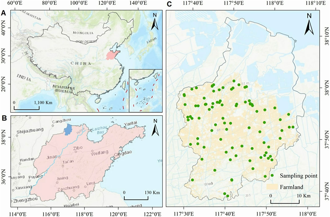
Figure 1. Geographic location of the study area and samples. (A) China; (B) Shandong Province; (C) Distribution of sampling points for farmland in Wudi County.

2.1.2 The technical flow of the study

To investigate the impact of combining multi-temporal images on SS inversion accuracy, this study implements the workflow illustrated in Figure 2. The methodology comprises five key steps: (1) collection and processing of both field-measured and remote sensing data; (2) identification of the optimal SS inversion time window and construction of combined images using various temporal integration strategies; (3) selection of SS-related spectral variables through multiple feature selection algorithms; (4) development and comparative analysis of inversion models; and (5) spatial mapping and validation of salinity distribution patterns.

Figure 2

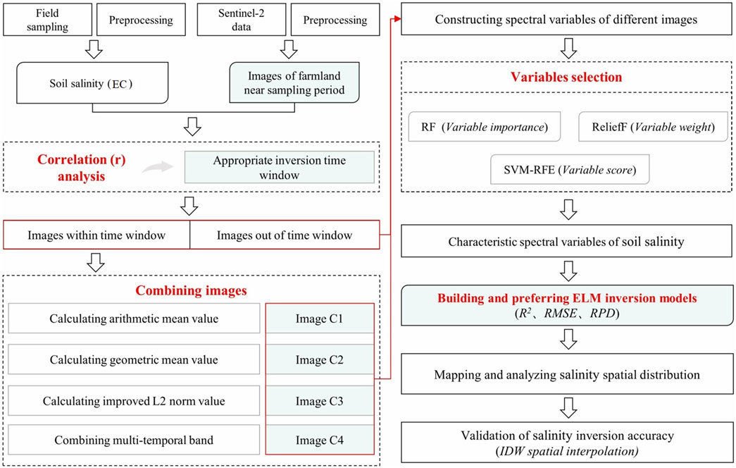
Figure 2. The workflow of this study.

2.2 Field sampling and data processing

Field sampling was conducted in the agricultural areas of Wudi County from September 5 to 10, 2020. During this period, cotton was in the boll splitting and shedding stage, while corn was in the grain filling and ripening stage, both exhibiting rapid growth variations. Additionally, frequent irrigation activities occurred due to high evapotranspiration rates. These conditions resulted in significant variations in soil and crop spectra, highlighting the importance of utilizing multi-temporal remote sensing imagery for effective SS monitoring. A total of 100 sampling sites were systematically distributed across the study area’s farmland, with precise locations determined using GPS coordinates. To minimize sampling errors and enhance data representativeness, a 2 m × 2 m sampling area was roughly established at each site, centered on the GPS coordinates. Following the five-point sampling method, soil electrical conductivity (EC, dS/m) measurements were taken at 0–10 cm depth using a portable soil conductivity meter (EC 110, Spectrum Technologies, United States) at the center and four corners of each sampling area. The average of the five measurements was calculated as the final EC value for each sampling point (Qi et al., 2022). To ensure data quality, outliers exceeding three times the average Mahalanobis distance (Chen et al., 2021) were removed using the Mahalanobis distance method, which accounts for the correlation between EC values and spectral data. This process resulted in 90 high-quality sample points retained for further analysis, with their spatial distribution illustrated in Figure 1C.

2.3 Multi-temporal images acquisition and processing

This study employed multispectral imagery from the Sentinel-2A and Sentinel-2B satellites, both equipped with the Multispectral Instrument (MSI), as the primary remote sensing data sources. These satellites provide 13 spectral bands spanning the visible to short-wave infrared spectrum, with consistent central wavelengths and spatial resolutions of 10, 20, and 60 m. While each individual satellite has a 10-day revisit period, the combined operation of Sentinel-2A and 2B reduces the temporal resolution to 5 days, enabling more detailed monitoring of agricultural activities and land cover dynamics. Focusing on the sampling period, six scenes of Level-2A images (geometrically and atmospherically corrected) with minimal cloud cover were acquired from the European Space Agency (ESA) website (https://dataspace.copernicus.eu) for three specific dates: September 1, 6, and 16 (Table 1). The coastal aerosol band (Band 1) and cirrus band (Band 10), primarily designed for nearshore water monitoring and cirrus cloud detection respectively, were excluded from the soil surface parameter inversion analysis. The remaining 11 spectral bands were resampled to a 10-meter resolution using three-dimensional convolution interpolation in the Sentinel Application Platform (SNAP). The six scenes were mosaicked into three single-temporal composite images (Image 1, Image 2, and Image 3) using ENVI 5.3 software. These images were subsequently cropped and classified by land use type to isolate farmland areas within the study region. Finally, spectral reflectance values corresponding to each sampling point were extracted using ArcGIS 10.2 software for subsequent analysis.

Table 1

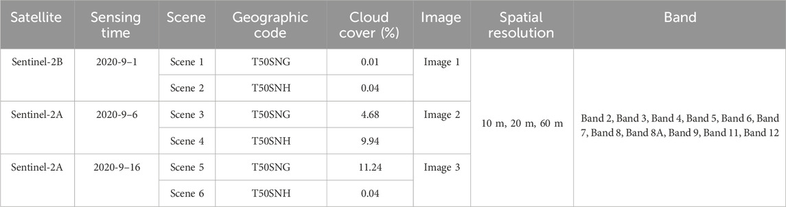
Table 1. Multi-temporal image information.

2.4 Image and spectral construction

2.4.1 Identification of the appropriate inversion window

The multi-temporal images contain extensive information, much of which is redundant for SS analysis. Therefore, the critical challenge lies in selecting the most relevant features that contribute to improving SS inversion precision. To address this, we employed two correlation-based metrics: (1) the individual correlation coefficient between each spectral band and SS, and (2) the total absolute correlation sum of all bands with SS. These metrics enable the identification of images containing the most significant salinity information. Based on the image acquisition times, an appropriate inversion window was determined. Images within this window were considered more suitable for extracting salinity information under varying environmental conditions, providing a robust foundation for subsequent image combination and analysis.

2.4.2 Reconstruction of combined-temporal images

To effectively capture salinity information from multiple images within the identified time window, four spectral combination strategies were designed from diverse perspectives to reconstruct combined-temporal images. These strategies comprise three arithmetic operations and one band combination approach. The specific procedures are as follows, where n represents the number of single-temporal images, and R_i denotes the reflectance of a specific spectral band across different periods.

(1) Combined-Temporal Image 1 (Image C1) – Arithmetic Mean of Multi-Temporal BandsThe arithmetic mean, a fundamental measure of central tendency, uniformly distributes spectral data to represent the average level of salinity spectra. The new reflectance (R) is calculated as shown in Equation 1.

$\mathit{R}=\frac{\mathbf{1}}{\mathit{n}}{\displaystyle \sum _{\mathit{i}=\mathbf{1}}^{\mathit{n}}}{\mathit{R}}_{\mathit{i}}(1)$

(2) Combined-Temporal Image 2 (Image C2) – Geometric Mean of Multi-Temporal BandsThe geometric mean is particularly effective for analyzing relative magnitudes and accommodating variations within the dataset. This approach mitigates the influence of outliers and provides a more robust representation of salinity spectrum variations. The new reflectance (R) is calculated as shown in Equation 2.

$\mathit{R}=\sqrt[\mathit{n}]{{\displaystyle \prod _{\mathit{i}=\mathbf{1}}^{\mathit{n}}}{\mathit{R}}_{\mathit{i}}}(2)$

(3) Combined-Temporal Image 3 (Image C3) – Improved L2 Norm of Multi-Temporal BandsThe L2 norm, widely employed in machine learning and data analysis, serves as a valuable tool in spectral analysis by compressing and centralizing salinity spectral information across different time points. To account for significant deviations in reflectance values, a correction coefficient of 1/n² is incorporated to enhance the calculation accuracy. The new reflectance (R) is calculated as shown in Equation 3.

$\mathit{R}=\sqrt{\frac{\mathbf{1}}{\mathit{n}}{\displaystyle \sum _{\mathit{i}=\mathbf{1}}^{\mathit{n}}}{{\mathit{R}}_{\mathit{i}}}^{\mathbf{2}}}(3)$

(4) Combined-Temporal Image 4 (Image C4) – Multi-Temporal Band Combination

The salinity features captured by different spectral bands exhibit multidimensional characteristics, with even the same band containing temporally varying salinity information. By analyzing the correlation between spectral bands and SS across multiple temporal images, the most sensitive bands for each spectral channel were identified and retained.

Using the four strategies described above, the new reflectance values for the 11 spectral bands were sequentially calculated. These values were then stacked in ENVI software and reconstructed into four combined-temporal images for subsequent analysis.

2.4.3 Construction of spectral indexes

To strengthen the relationship between spectral data and measured soil EC values, 34 spectral indexes were derived for each image to directly or indirectly represent salinity levels (Ivushkin et al., 2017; Guo et al., 2019). These indexes include 15 vegetation indexes, such as the Salinity Index 1 (SI1) and Salinity Index 2 (SI2), and 18 salinity indexes, including the Normalized Difference Vegetation Index (NDVI) and Difference Vegetation Index (DVI). Additionally, red-edge bands, which exhibit heightened sensitivity to salinity in vegetated areas (Kaplan and Avdan, 2019), were incorporated to enhance salinity characterization, exemplified by the Salinity Index 1 Red Edge 1 (SI1re1). The calculation formulas for these indexes were detailed in Table 2.

Table 2

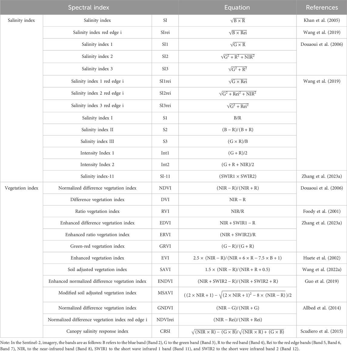
Table 2. Spectral indexes calculation equations.

2.5 Statistical method

2.5.1 Selection of SS characteristic spectral variables

Variable selection represents a critical step in data modeling and machine learning processes, primarily aimed at identifying the most influential variables for enhancing model predictive performance. Variable selection methods can be broadly categorized into three types: wrapper, filter, and embedded approaches (Chandrashekar and Sahin, 2014). In this study, we employed three distinct algorithms—Random Forest (RF), ReliefF, and Support Vector Machine Recursive Feature Elimination (SVM-RFE)—to identify key variables from spectral datasets derived from both single-temporal and combined-temporal images. These datasets included 11 spectral bands and 34 spectral indexes. These algorithms effectively reduce data redundancy (Wang et al., 2019) and streamline the construction of inversion models. All methods were implemented using MATLAB R2016b software.

2.5.1.1 RF selection algorithm

RF variable selection is an embedded ensemble learning algorithm that constructs multiple decision trees through random sampling of both data instances and variables. This method inherently evaluates the importance of each variable within the decision tree framework and identifies the most relevant features (Tan et al., 2023). The algorithm’s key parameter is the number of trees, which was set to 150 in this study, with a minimum of five leaf nodes per tree.

2.5.1.2 ReliefF selection algorithm

ReliefF is a widely recognized filter-based variable selection algorithm, particularly effective for identifying significant variables in high-dimensional datasets. In regression applications, ReliefF assesses a variable’s contribution by analyzing weight value differences between each sample and its nearest similar samples (neighbors) (Xi et al., 2023). A greater difference in weight values relative to the target variable indicates a stronger impact of the variable. In this study, the algorithm parameters were configured with six nearest neighbors and 50 randomly selected samples.

2.5.1.3 SVM-RFE selection algorithm

SVM-RFE is a wrapper-based variable selection algorithm that iteratively trains a support vector machine while progressively eliminating variables with minimal impact on model performance (Guo et al., 2022). In this study, the algorithm was configured with the following parameters: an initial score of 45 for each spectral variable, where the score for a variable removed in the nth iteration was calculated as 45 - n until no variables remained. The penalty parameter was set to 4, the radial basis function was employed as the kernel function with a bandwidth of 0.2, and epsilon was set to 0.01.

To ensure comparability across the results from the three algorithms, the variable importance values generated by RF, the variable weights from ReliefF, and the variable scores from SVM-RFE were normalized to a common scale of variable importance. These normalized values served as consistent evaluation metrics for subsequent analysis and comparative assessment of the results.

2.5.2 Building and preferring of SS inversion model

This study employed 90 measured salinity samples and selected spectral variables, divided into training and test sets at a 2:1 ratio. The Extreme Learning Machine (ELM) algorithm, implemented in MATLAB R2016b, was used to develop SS inversion models. The ELM network architecture consists of an input layer, at least one hidden layer, and an output layer. While the weights between the input and hidden layers are randomly initialized, the weights between the hidden and output layers are systematically trained. This streamlined training process significantly enhances the model’s learning efficiency and generalization capabilities, making ELM a widely adopted method in soil property analysis (Acar et al., 2020; Zhao et al., 2022). In this study, the number of neurons in the input layer corresponds to the number of input variables, while the hidden layer is configured with 10 neurons using a sigmoid activation function. The output layer contains a single neuron.

Model performance was evaluated on both training and test sets using the Coefficient of Determination (R²) and Root Mean Square Error (RMSE), where higher R² values and lower RMSE values indicate superior model performance. Additionally, the Relative Percentage Deviation (RPD) was calculated for the test set to further assess the model’s generalization ability. Based on established criteria (Wang Y. et al., 2022), model predictive capability is classified as poor when RPD <1.4, moderate when 1.4 ≤ RPD <1.8, and excellent when RPD ≥1.8 (Wang Y. et al., 2022).

2.5.3 Mapping and validation of SS spatial distribution

Using the best-performing inversion model, SS was mapped for the study area. Referring to the classification criteria for salinized soils proposed by the U.S. Salinity Laboratory staff (Richards, 1954), soil salinity maps were classified into the following categories of criteria: Salinity effects mostly negligible (EC = 0–2 dS/m), Yields of very sensitive crops maybe restricted (EC = 2–4 dS/m), Yields of many crops restricted (EC = 4–8 dS/m), Only tolerant crops yield satisfactorily (EC = 8–16 dS/m), and Only a few very tolerant crops yield satisfactorily (EC ≥ 16 dS/m). Furthermore, to validate the remote sensing model’s accuracy, we conducted a comparative analysis with geostatistical interpolation results. Specifically, an inverse distance weighting (IDW) map was generated using the limited field sampling data from the study area (Chen et al., 2021). This IDW-derived map was then systematically compared with the remote sensing inversion map through spatial statistical evaluation.

3 Results

3.1 Description of sample point salinity

Figure 3 presents the statistical characteristics of SS for samples collected in Wudi County. The EC values ranged from 0.37 to 6.25 dS/m (mean = 1.60 dS/m). Notably, the training set (n = 60, mean EC = 1.66 dS/m) and test set (n = 30, mean EC = 1.77 dS/m) exhibited nearly identical statistical distributions to the entire dataset. Crucially, no statistically significant differences were detected in the interquartile ranges among the three datasets, confirming homogeneous sample distribution patterns. This stratification consistency ensured representative data partitioning, thereby effectively reducing potential estimation bias during both model calibration and validation phases.

Figure 3

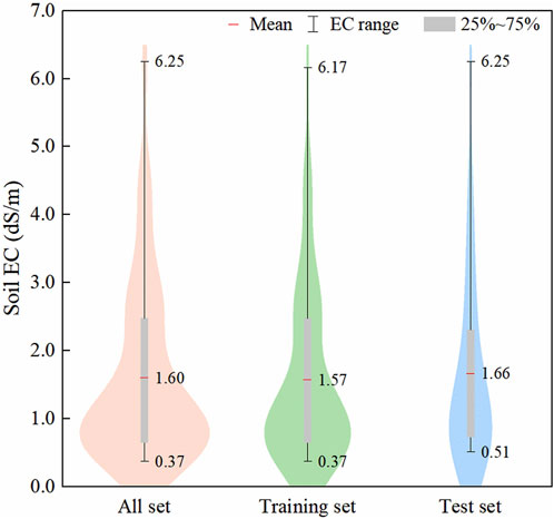
Figure 3. Soil EC statistics of the sample sets.

3.2 Appropriate SS inversion time windows and image spectral construction

To determine an appropriate inversion time window, correlation analysis was conducted as shown in Figure 4. The temporal correlation patterns between spectral bands and SS showed general consistency across the three single-date images. With increasing wavelengths of Sentinel-2 bands, the correlation with SS transitioned from positive to negative before returning to positive values in longer wavelengths. Maximum positive correlations were observed in Band 4 (Red) and Band 5 (Red Edge 1), while peak negative correlations centered on Band 8 (Near Infrared). Notably, Image two demonstrated the strongest positive correlations (highlighted by solid red borders), particularly in Bands 2–5 (Visible to Red Edge1) and Bands 11–12 (Shortwave Infrared). Conversely, Image three showed the most pronounced negative correlations (highlighted by solid red borders), primarily in Bands 6–9 (Red Edge to Near Infrared). The enhanced sensitivity of these specific bands in Images two and three compared to equivalent bands in other images suggests that the spectral reflectance-SS relationship is not static. Environmental factors such as soil moisture, organic matter content, and land cover may affect this relationship and render it variable over time.

Figure 4

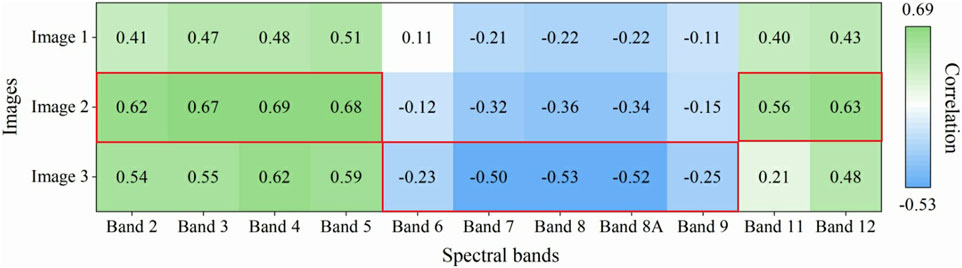
Figure 4. The correlation between single-temporal spectra and SS.

The total correlation between SS and all bands was quantified for each image. Image one showed correlations ranging from −0.22 to 0.51, with a cumulative absolute correlation sum of 3.57. Image two demonstrated a broader correlation interval (−0.36–0.69) and a higher cumulative sum (5.14), indicating enhanced salinity sensitivity. Image three exhibited correlations from −0.53 to 0.62, with a cumulative sum of 5.02. This analysis confirms that Images two and three exhibit significantly stronger correlations with SS than Image 1, both at individual band and full-image scales. Consequently, the period spanning September 6–16 was identified as the appropriate time window for SS inversion. Subsequently, Images two and three within the window are reconstructed using the four methods mentioned earlier to obtain the combined-temporal images. In addition, not all proximate images can be effectively combined; rigorous time window analysis remains critical for identifying suitable candidates.

3.3 SS informativeness of combined-temporal images

To assess whether the spectral informativeness of SS in the combined-temporal images was enhanced, a correlation analysis between the images and SS was conducted, as illustrated in Figure 5. The combination of Image two and Image three using four distinct strategies led to a significant increase in the correlation between the combined-temporal images and SS, compared to the individual images within the time window. Specifically, the total absolute correlation for the 11 spectral bands in Image C1 increased by 0.12–0.24, in Image C2 by 0.06–0.18, in Image C3 by 0.23–0.35, and Image C4 demonstrated the most substantial improvement, ranging from 0.74 to 0.86. These results clearly indicate that combining images from the appropriate time window enhances correlation and further enriches the information content related to salinity.

Figure 5

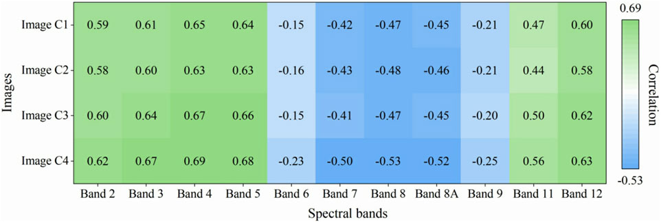
Figure 5. The correlation between combined-temporal spectra and SS.

The multi-temporal band combination strategy (Image C4) proved to be the most effective, as it integrated the most relevant bands from both Image two and Image 3. In contrast, the arithmetic-based combination strategies (Images C1, C2, and C3) exhibited more modest improvements. While the overall performance of these images improved, certain bands displayed a slight reduction in sensitivity. For instance, in Image C1, the correlation of Band five was higher than in Image three but slightly lower than in Image 2, whereas Band eight showed the opposite trend, being higher than in Image two but lower than in Image 3.

3.4 The characteristic spectral variable of SS

To mitigate the impact of variable quantity on model performance, this study fixed the number of output variables at six during the variable selection process, a point at which modeling effectiveness became relatively stable. Figure 6 illustrates the top six spectral variables prioritized by three feature selection algorithms across the seven image datasets.

Figure 6

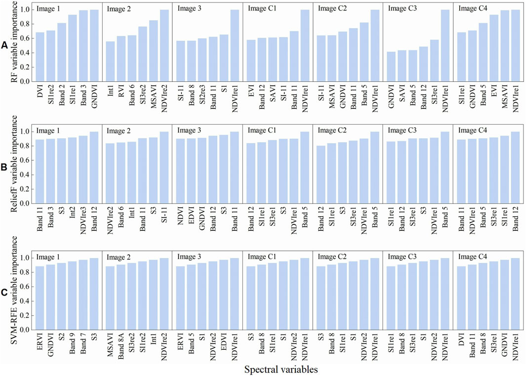
Figure 6. Characteristic spectral variables. Variable output results for (A) RF, (B) ReliefF and (C) SVM-RFE.

For different variable selection algorithms, distinct methods exhibited significant differences. The RF algorithm demonstrated broader coverage in variable selection, particularly emphasizing vegetation indices that indirectly conveyed SS information, such as NDVIre1, GNDVI, and MSAVI, as well as reflectance in the Red Edge one band (Band 5) and the Shortwave Infrared one band (Band 11). The combined selection frequency of these related variables reached 42.9%. In contrast, the ReliefF algorithm prioritized reflectance in the Shortwave Infrared bands (Bands 11 and 12) alongside various salinity indices that directly characterized salinity information, including S3, SI1re1, and SI3re1, achieving a total selection frequency as high as 57.1%. The SVM-RFE algorithm showed a preference for both vegetation indices (NDVIre1 and NDVIre2) and salinity indices (S1, S2, and SI1re1), with the total selection frequency of these variables reaching 47.6%. These findings highlight that, due to differences in their selection mechanisms, the three algorithms exhibited distinct preferences and focal points in feature variable selection.

Regarding different images, particularly before and after image combination, the variables selected by the three algorithms were relatively dispersed in single-temporal images, with limited commonalities among the spectral variables of different images. The most frequently selected variables included GNDVI, Int1, NDVIre2, Band 11, S3, and Band 12, with a total selection frequency of only 33.3% in single-temporal images. Conversely, for all combined-temporal images, the selected variables were more concentrated, with the most frequently selected spectral variables being NDVIre1, SI1re1, Band 5, SI1re3, and Band 12, yielding a selection frequency of 55.6%. This indicates a significant shift in spectral variable selection before and after image combination, reflecting changes in the spectral data related to SS information content.

A cross-selection analysis was conducted to identify spectral variables consistently explaining soil salinization across different images and selection algorithms. Supplementary Figure S1 in the supplementary material presents the cumulative importance of all variables identified in this study. NDVIre1, GNDVI, SI1re1, S3, SI3re1, and MSAVI ranked highest in importance, contributing significantly to the interpretation of SS in vegetated regions, particularly NDVIre1. These results are likely more reliable than single-variable selection based on a single image, as they demonstrate the stability and robustness of the selected variables across different time points and algorithmic approaches. Notably, many key variables included indices derived from red edge bands, underscoring their strong potential for SS monitoring.

3.5 Optimal SS quantitative inversion model

Using the characteristic spectral variables (shown in Figure 6) and SS data, ELM SS inversion models were developed and validated. The results are presented in Figure 7.

Figure 7

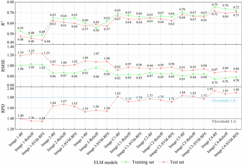
Figure 7. Quantitative remote sensing SS inversion models.

3.5.1 Evaluation of model performance based on different images

Analysis of models built using different images revealed that those based on single-temporal images produced the following performance metrics on the test set: R² values ranged from 0.44 to 0.62, RMSE values ranged from 1.00 to 1.23 dS/m, and RPD values ranged from 1.35 to 1.67. These results indicate moderate model performance, suggesting room for improvement. When combining Image two and Image 3, models built with the combined-temporal images showed significant improvements in both the training and test sets. Specifically, validated R² values increased to between 0.62 and 0.72, RMSE values decreased to between 0.87 and 0.98 dS/m, and RPD values rose to between 1.71 and 1.93. Compared to single-temporal models, the combined-temporal models exhibited R² increases ranging from 0.02 to 0.36, RMSE reductions from 0.02 to 0.42 dS/m, and RPD increases from 0.04 to 0.58. These findings highlight the significant improvements in accuracy achieved by combining images, enhancing the model’s effectiveness for remote sensing SS predictions.

Figures 8A–C provide the performance statistics for different images on the test set. In a comprehensive evaluation of individual image performances, the ELM model utilizing Image C4 exhibited outstanding results on both the training and validation datasets. The validated R² values ranged from 0.69 to 0.72, RMSE values ranged from 0.87 to 0.89 dS/m, and RPD values ranged from 1.87 to 1.93, all exceeding the threshold of 1.8. Compared to other combined-temporal models, the Image C4 model achieved a higher mean RPD, with an increase of 0.09–0.15, and outperformed the single-temporal models with a mean RPD increase of 0.25–0.53. This suggests that Image C4 is the most effective for predicting SS with minimal prediction errors. Following Image C4, the model based on Image C3 also demonstrated strong performance, with RPD values ranging from 1.77 to 1.84. Other models ranked in descending order of prediction effectiveness include Image C1 (RPD = 1.72–1.82), Image C2 (RPD = 1.71–1.77), Image 2 (RPD = 1.63–1.67), Image 3 (RPD = 1.53–1.56), and Image 1 (RPD = 1.35–1.40). Notably, most models constructed using Image one had RPDs below the threshold of 1.4, R² values ranging from 0.44 to 0.48, and RMSE values between 1.19 and 1.23, indicating relatively poor performance.

Figure 8

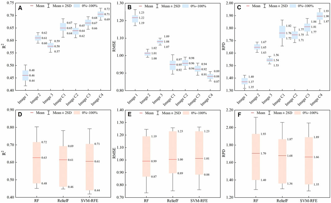
Figure 8. Validated model performance statistics for image and variable selection algorithms. (A) R², (B) RMSE and (C) RPD for different images; (D) R², (E) RMSE and (F) RPD for different algorithms.

3.5.2 Evaluation of model performance based on variable selection algorithms

Figures 8D-F provide the performance statistics for different images on the test set. Among the models developed using various variable selection algorithms, the RF algorithm demonstrated the highest performance for SS prediction. Models based on RF variable selection achieved R² values between 0.48 and 0.72, RMSE values ranging from 0.87 to 1.19 dS/m, and RPD values between 1.40 and 1.93 on the test set. Compared to other variable selection methods, the mean RPD of RF-based models was 0.02–0.04 higher. Following RF, the SVM-RFE algorithm ranked second (R² = 0.44–0.71, RMSE = 0.88–1.23, RPD = 1.35–1.89), while the ReliefF algorithm ranked third (R² = 0.46–0.69, RMSE = 0.89–1.23, RPD = 1.36–1.87). Interestingly, although SVM-RFE outperformed ReliefF in terms of RPD variation range when considering the mean metric, the mean RPD for SVM-RFE was 1.66, which was slightly lower than the 1.68 of the ReliefF algorithm. This suggests that, while individual models based on the SVM-RFE variable selection algorithm performed better, the overall performance of models using the ReliefF algorithm was superior.

3.5.3 Evaluation of model performance based on images and variable selection methods

From the above analysis, the models with an RPD exceeding the threshold of 1.8 include the Image C4-RF-ELM, Image C4-ReliefF-ELM, and Image C4-SVM-RFE-ELM models. All of these models utilize the optimal predictive Image C4, suggesting that the choice of image has a more significant impact on model performance than the selection of the variable selection method. Specifically, the models that combine Image C4 with the RF variable selection algorithm show the best fit on both the training and validation datasets, with the lowest prediction errors. For the test set, the R² value reaches 0.72, the minimum RMSE is 0.87 dS/m, and the RPD peaks at 1.93, with a scatter plot that closely clusters around the 1:1 line (Supplementary Figure S2). This model was then used to map regional SS. Additionally, the models using SVM-RFE and ReliefF as variable selection algorithms achieved RPD values of 1.87 and 1.89, respectively, with their scatter plots also showing a high degree of concentration. These results indicate that these models also perform well in SS inversion and provide satisfactory prediction accuracy.

3.6 SS spatial distribution analysis and validation

3.6.1 Spatial distribution analysis

The Image C4-RF-ELM model was used to map the SS distribution in the study area (Figure 9A) and to classify the proportion of farmland at each salinity level (Figure 10). The SS inversion map of Wudi County reveals a clear salinity gradient, increasing from the southwestern areas towards the northeastern coastal low-lying regions, which aligns with the actual environmental conditions. Approximately 53.3% of the farmland had soil salinity that had a negligible effect on crops, primarily distributed around southwestern townships, southeastern sectors, and riparian zones in the western region. In contrast, 46.7% of cultivated lands exhibited varying degrees of salinization, predominantly concentrated in central areas and northeastern coastal regions where seawater intrusion has created scattered saline-alkali patches. Notably, 33.1% of farmland faced productivity constraints for salt-sensitive crops, 8.1% significantly inhibited yields for most crops, while the remaining 5.5% maintained satisfactory productivity only for salt-tolerant cultivars.

Figure 9

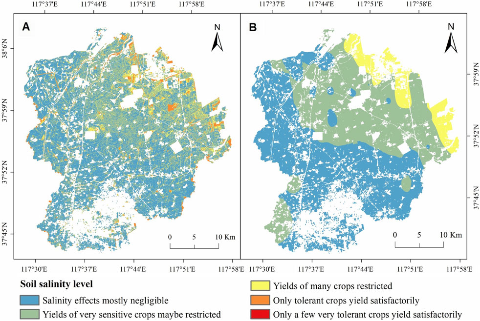
Figure 9. Spatial distribution of SS in the study area. (A) Remote sensing inversion map; (B) IDW interpolation map.

Figure 10

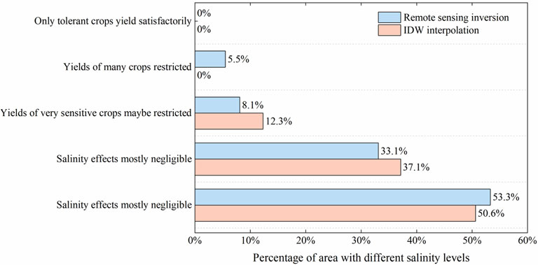
Figure 10. Percentage of area for each SS level in the study area.

3.6.2 Verification of inversion result

The IDW interpolation results and classification statistics are shown in Figures 9B, 10. The IDW interpolation and remote sensing inversion results indicate that the spatial distribution patterns of salinized farmland exhibit no significant discrepancies. Both maps, for instance, reveal a gradient of increasing salinization intensity extending from the southwest to the northeast. However, the remote sensing approach estimated a smaller total area of saline-alkali soils while demonstrating a stronger capability in delineating more refined spatial distribution patterns of salinization. In conclusion, the findings demonstrate that the remote sensing inversion model, based on multi-temporal combined imagery, provides precise and reliable predictions of salinized soil distribution patterns in the study region. This methodology offers valuable insights for optimizing local agricultural cultivation strategies and crop allocation.

4 Discussion

4.1 Validity of combined-temporal images

This study demonstrated that combining multi-temporal remote sensing images near the sampling period significantly enhanced the precision and stability of SS inversion compared to single-image analysis. This improvement can be attributed to three key factors.

Firstly, in September, frequent agricultural activities—such as cultivation, irrigation, and natural precipitation—caused short-term fluctuations in stress factors like soil moisture (Fathololoumi et al., 2020). These changes affected the condition and spectral responses of saline soils (Metternicht and Zinck, 2003). Figure 11 illustrates the mean reflectance change across all sample points between two images taken 10 days apart within the appropriate inversion time window. Heavy rainfall before the second image (weather data are shown in Supplementary Table S1 of the supplementary material) significantly altered land surface moisture content and spectral characteristics, particularly in Bands 6–9. This shift may explain why Near Infrared bands in the September 16 image correlated more strongly with salinity than those in the September 6 image. Such variability underscores the importance of accounting for temporal and environmental factors in spectral data for soil salinity assessment, reinforcing the value of multi-temporal analysis in capturing dynamic salinity spectral characteristics. This approach aligns with the broader trend of using multi-temporal imagery for agricultural information extraction, such as wheat growth monitoring (Qu et al., 2021; Feng et al., 2024). Similarly, in SS prediction, capturing spectral variations at different stages is essential. By integrating multi-temporal images and applying effective feature selection methods, external influences like weather and human activities can be filtered out (Tagarakis and Ketterings, 2017), isolating true salinity information. This method enables more precise retrieval of spectral data for assessing salinization (Lobell et al., 2007; Lobell et al., 2010; Furby et al., 2010; Wu et al., 2014; Whitney et al., 2018; Fathololoumi et al., 2020; Wang et al., 2023). Our study confirmed that incorporating temporal spectral changes significantly improves SS information extraction.

Figure 11

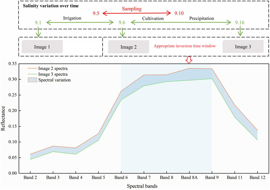
Figure 11. Spectral variations within appropriate time window due to environmental factors.

Secondly, previous studies have primarily relied on long-time-series remote sensing images, which often involve significant workloads and operational complexity. While cloud-based remote sensing platforms such as Google Earth Engine accelerate processing workflows, directly synthesizing long-time-series images without selecting an appropriate inversion window may overlook abrupt soil salinity changes, introducing information unrelated to soil salinity. Research has shown that the shorter the time interval between image acquisition and sampling, the higher the mapping accuracy (Luo et al., 2023). Based on this, our study fully considers the temporal variability of soil salinity spectra by selecting only images captured within a week before or after the sampling period. This approach enhances operational feasibility while ensuring a comprehensive capture of soil salinity dynamics within the timeframe. By minimizing the redundancy of non-salinity-related factors caused by the time lag between image acquisition and sampling, this method improves the accuracy of real-time SS monitoring models.

Finally, this study introduces an innovative multi-temporal band combination strategy that integrates the most salinity-sensitive bands from each spectral channel across multiple spatiotemporal images, offering the most robust salinity expression capability—an aspect not previously addressed in soil salinity research. Compared to the three arithmetic-based image generation strategies used in this study, the proposed method demonstrated superior performance. This is mainly because arithmetic calculations typically yield salinity information that falls between two sets of band data. While all bands undergo collective enhancement, individual bands may not reach their optimal performance, thereby limiting overall effectiveness.

4.2 Comparison of spectral variable selecting algorithms

The selection of effective characteristic spectral variables is crucial for ensuring the accuracy of SS prediction models, as different selection methods can significantly influence model performance (Wang Y. et al., 2022). In this study, three variable selection algorithms, each based on distinct theoretical frameworks, were employed to identify characteristic spectral variables for salinity prediction. The RF algorithm, known for its robustness (Genuer et al., 2010) and high tolerance to noise and outliers, is particularly effective in complex data environments, though it may require extensive training time when handling numerous features. The SVM-RFE algorithm, a wrapper selection method, efficiently identifies the most informative features with fewer variables, yet its effectiveness heavily depends on parameter settings and involves considerable computational costs (Li et al., 2021). The ReliefF algorithm, proficient at detecting interactions between features, operates efficiently but is more sensitive to noise and less effective at eliminating redundant features (You et al., 2014). In remote sensing, atmospheric factors such as water vapor can interfere with spectral data, particularly in the visible-near-infrared spectra of soils, where noise may obscure actual salinity information (Taghdis et al., 2022). In this context, the RF algorithm demonstrated superior performance compared to the other two algorithms due to its high resilience to noise, consistent with prior research findings. For example, Wang et al. (2019) also concluded that the RF algorithm is highly effective in identifying characteristic spectral variables for SS. A limitation of this study is the lack of model validation for the cross-variable results obtained from different algorithms. Future research should prioritize addressing this limitation to determine whether combining spectral variables selected by different algorithms enhances model robustness.

4.3 Selection of multi-temporal images

This study aimed to enhance salinity mapping precision by extracting salinity information from dynamic, multi-temporal spectral data closely aligned with the sampling period. MODIS satellites, with their 1-day temporal resolution, were initially considered but deemed unsuitable due to their insufficient spatial resolution (250–1,000 m) for the fragmented study area. Instead, Sentinel-2 imagery, offering a 5-day temporal resolution and spatial resolutions of 10–60 m, was selected for its precision. To align with the sampling period (5–10 September 2020), Sentinel-2 images from 1 September (pre-sampling), 6 September (during sampling), and 11 September (post-sampling) were initially chosen as Image 1, Image 2, and Image 3, respectively. However, due to cloud cover on 11 September, the image from 16 September was used as a replacement. Analysis revealed that the pre-sampling image (1 September) exhibited a weak correlation with SS, and its inclusion in image combinations reduced salinity-related information. Consequently, the period from six to 16 September was identified as the optimal inversion time window for exploring image combination strategies. Additionally, the three single-temporal images were combined using the improved L2 paradigm strategy. However, the inversion results were less accurate compared to those obtained from image combinations within the identified inversion window, even when using the same variable selection algorithm. This suggests that not all images near the sampling period are suitable for combination. Exploring an appropriate time window effectively enhances accuracy while reducing data processing efforts. Future studies should assess whether using imagery from dates even closer to the sampling period, such as 11 September, could further improve inversion accuracy.

5 Conclusion

This study utilized three Sentinel-2 MSI time-series images captured near the sampling period to determine the optimal inversion time window for SS mapping. Four spectral combination strategies—arithmetic mean, geometric mean, improved L2 norm, and spectral band combination—were applied to merge multi-temporal images within this window. Spectral variables were selected from both pre-and post-combination images using RF, ReliefF, and SVM-RFE algorithms and then integrated with the ELM regression algorithm to develop SS inversion models. The results demonstrated that combining multi-temporal images near the sampling period significantly improved the correlation between SS and spectral data, enhancing inversion accuracy. Selecting images within an optimal time window proved more efficient than using all available images. Models based on multi-temporal band combination images exhibited superior validation performance (R² = 0.69–0.72, RMSE = 0.87–0.89 dS/m, RPD = 1.87–1.93), with mean RPD values surpassing those of single-temporal models by 0.25–0.53. Among the spectral variable selection methods, models using the RF algorithm performed best (validation R² = 0.48–0.72, RMSE = 0.87–1.19 dS/m, RPD = 1.40–1.93), achieving mean RPD values 0.02–0.04 higher than other selection algorithms. The most critical SS-related spectral variables identified through cross-selection included NDVIre1, GNDVI, SI1re1, S3, SI3re1, and MSAVI, with the red edge one band making a particularly significant contribution. The best-performing model, incorporating a multi-temporal band combination image with RF-based variable selection, achieved excellent results (training R² = 0.75, RMSE = 0.75 dS/m; validation R² = 0.72, RMSE = 0.87 dS/m, RPD = 1.93). The inversion map revealed a distinct southwest-to-northeast salinity gradient, with 46.7% of farmland exhibiting varying degrees of salinization that impact crop yields. These findings provide valuable insights for large-scale SS spatial mapping, advancing precision and smart agriculture, and offering accurate data for managing salinized farmland and its ecological environment.

Data availability statement

The raw data supporting the conclusions of this article will be made available by the authors, without undue reservation.

Author contributions

CD: Conceptualization, Formal Analysis, Methodology, Software, Writing–original draft, Writing–review and editing. YZ: Investigation, Methodology, Writing–review and editing. CH: Data curation, Visualization, Writing–review and editing. HC: Funding acquisition, Supervision, Writing–review and editing. PL: Investigation, Resources, Writing–review and editing.

Funding

The author(s) declare that financial support was received for the research and/or publication of this article. This research was supported by the National Natural Science Foundation of China (grant number 42477523); the Natural Science Foundation of Shandong Province (grant number ZR2023MD033); the National Key Research and Development Program of China (grant number 2023YFD2303304).

Acknowledgments

Thanks to the ESA for support with the Sentinel-2 MSI images.

Conflict of interest

The authors declare that the research was conducted in the absence of any commercial or financial relationships that could be construed as a potential conflict of interest.

Generative AI statement

The authors declare that no Generative AI was used in the creation of this manuscript.

Publisher’s note

All claims expressed in this article are solely those of the authors and do not necessarily represent those of their affiliated organizations, or those of the publisher, the editors and the reviewers. Any product that may be evaluated in this article, or claim that may be made by its manufacturer, is not guaranteed or endorsed by the publisher.

Supplementary material

The Supplementary Material for this article can be found online at: https://www.frontiersin.org/articles/10.3389/fenvs.2025.1533419/full#supplementary-material

References

Abbas, A., Khan, S., Hussain, N., Hanjra, M. A., and Akbar, S. (2013). Characterizing soil salinity in irrigated agriculture using a remote sensing approach. Phys. Chem. Earth Parts ABC 55–57, 43–52. doi:10.1016/j.pce.2010.12.004

PubMed Abstract | CrossRef Full Text | Google Scholar

Abuelgasim, A., and Ammad, R. (2019). Mapping soil salinity in arid and semi-arid regions using Landsat 8 OLI satellite data. Remote Sens. Appl. Soc. Environ. 13, 415–425. doi:10.1016/j.rsase.2018.12.010

CrossRef Full Text | Google Scholar

Acar, H., Ozerdem, M. S., and Acar, E. (2020). Soil moisture inversion via semiempirical and machine learning methods with full-polarization radarsat-2 and polarimetric target decomposition data: a comparative study. IEEE Access 8, 197896–197907. doi:10.1109/ACCESS.2020.3035235

CrossRef Full Text | Google Scholar

Allbed, A., Kumar, L., and Sinha, P. (2014). Mapping and modelling spatial variation in soil salinity in the Al hassa oasis based on remote sensing indicators and regression techniques. REMOTE Sens. 6, 1137–1157. doi:10.3390/rs6021137

CrossRef Full Text | Google Scholar

Ayaz, M., Ammad-Uddin, M., Sharif, Z., Mansour, A., and Aggoune, E.-H. M. (2019). Internet-of-Things (IoT)-Based smart agriculture: toward making the fields talk. IEEE ACCESS 7, 129551–129583. doi:10.1109/ACCESS.2019.2932609

CrossRef Full Text | Google Scholar

Bian, L., Wang, J., Liu, J., and Han, B. (2021). Spatiotemporal changes of soil salinization in the Yellow River Delta of China from 2015 to 2019. Sustainability 13, 822. doi:10.3390/su13020822

CrossRef Full Text | Google Scholar

Bouaziz, M., Matschullat, J., and Gloaguen, R. (2011). Improved remote sensing detection of soil salinity from a semi-arid climate in Northeast Brazil. Comptes Rendus Geosci. 343, 795–803. doi:10.1016/j.crte.2011.09.003

CrossRef Full Text | Google Scholar

Chandrashekar, G., and Sahin, F. (2014). A survey on feature selection methods. Comput. Electr. Eng. 40, 16–28. doi:10.1016/j.compeleceng.2013.11.024

CrossRef Full Text | Google Scholar

Chen, H., Ma, Y., Zhu, A., Wang, Z., Zhao, G., and Wei, Y. (2021). Soil salinity inversion based on differentiated fusion of satellite image and ground spectra. Int. J. Appl. Earth Obs. Geoinformation 101, 102360. doi:10.1016/j.jag.2021.102360

CrossRef Full Text | Google Scholar

Dong, R., and Na, X. (2021). Quantitative retrieval of soil salinity using landsat 8 OLI imagery. Appl. Sci.-Basel 11, 11145. doi:10.3390/app112311145

CrossRef Full Text | Google Scholar

Douaoui, A. E. K., Nicolas, H., and Walter, C. (2006). Detecting salinity hazards within a semiarid context by means of combining soil and remote-sensing data. Geoderma 134, 217–230. doi:10.1016/j.geoderma.2005.10.009

CrossRef Full Text | Google Scholar

Fathololoumi, S., Vaezi, A. R., Alavipanah, S. K., Ghorbani, A., Saurette, D., and Biswas, A. (2020). Improved digital soil mapping with multitemporal remotely sensed satellite data fusion: a case study in Iran. Sci. Total Environ. 721, 137703. doi:10.1016/j.scitotenv.2020.137703

PubMed Abstract | CrossRef Full Text | Google Scholar

Feng, Y., Chen, B., Liu, W., Xue, X., Liu, T., Zhu, L., et al. (2024). Winter wheat mapping in Shandong Province of China with multi-temporal sentinel-2 images. Appl. Sci.-Basel 14, 3940. doi:10.3390/app14093940

CrossRef Full Text | Google Scholar

Foody, G. M., Cutler, M. E., McMorrow, J., Pelz, D., Tangki, H., Boyd, D. S., et al. (2001). Mapping the biomass of Bornean tropical rain forest from remotely sensed data. Glob. Ecol. Biogeogr. 10, 379–387. doi:10.1046/j.1466-822X.2001.00248.x

CrossRef Full Text | Google Scholar

Furby, S., Caccetta, P., and Wallace, J. (2010). Salinity monitoring in western Australia using remotely sensed and other spatial data. J. Environ. Qual. 39, 16–25. doi:10.2134/jeq2009.0036

PubMed Abstract | CrossRef Full Text | Google Scholar

Genuer, R., Poggi, J.-M., and Tuleau-Malot, C. (2010). Variable selection using random forests. Pattern Recognit. Lett. 31, 2225–2236. doi:10.1016/j.patrec.2010.03.014

CrossRef Full Text | Google Scholar

Guo, B., Han, B., Yang, F., Fan, Y., Jiang, L., Chen, S., et al. (2019). Salinization information extraction model based on VI-SI feature space combinations in the Yellow River Delta based on Landsat 8 OLI image. Geomat. Nat. Hazards Risk 10, 1863–1878. doi:10.1080/19475705.2019.1650125

CrossRef Full Text | Google Scholar

Guo, J., Wang, K., and Jin, S. (2022). Mapping of soil pH based on SVM-RFE feature selection algorithm. Agron. Basel 12, 2742. doi:10.3390/agronomy12112742

CrossRef Full Text | Google Scholar

He, Y., Zhang, Z., Xiang, R., Ding, B., Du, R., Yin, H., et al. (2023). Monitoring salinity in bare soil based on Sentinel-1/2 image fusion and machine learning. Infrared Phys. Technol. 131, 104656. doi:10.1016/j.infrared.2023.104656

CrossRef Full Text | Google Scholar

Huete, A., Didan, K., Miura, T., Rodriguez, E. P., Gao, X., and Ferreira, L. G. (2002). Overview of the radiometric and biophysical performance of the MODIS vegetation indices. Remote Sens. Environ. 83, 195–213. doi:10.1016/S0034-4257(02)00096-2

CrossRef Full Text | Google Scholar

Ivushkin, K., Bartholomeus, H., Bregt, A. K., and Pulatov, A. (2017). Satellite thermography for soil salinity assessment of cropped areas in Uzbekistan. Land Degrad. Dev. 28, 870–877. doi:10.1002/ldr.2670

CrossRef Full Text | Google Scholar

Ivushkin, K., Bartholomeus, H., Bregt, A. K., Pulatov, A., Franceschini, M. H. D., Kramer, H., et al. (2019a). UAV based soil salinity assessment of cropland. Geoderma 338, 502–512. doi:10.1016/j.geoderma.2018.09.046

CrossRef Full Text | Google Scholar

Ivushkin, K., Bartholomeus, H., Bregt, A. K., Pulatov, A., Kempen, B., and de Sousa, L. (2019b). Global mapping of soil salinity change. Remote Sens. Environ. 231, 111260. doi:10.1016/j.rse.2019.111260

CrossRef Full Text | Google Scholar

Kaplan, G., and Avdan, U. (2019). Evaluating the utilization of the red edge and radar bands from sentinel sensors for wetland classification. Catena 178, 109–119. doi:10.1016/j.catena.2019.03.011

CrossRef Full Text | Google Scholar

Khan, N. M., Rastoskuev, V. V., Sato, Y., and Shiozawa, S. (2005). Assessment of hydrosaline land degradation by using a simple approach of remote sensing indicators. Agric. Water Manag. 77, 96–109. doi:10.1016/j.agwat.2004.09.038

CrossRef Full Text | Google Scholar

Li, G., Wang, C., Zhang, D., and Yang, G. (2021). An improved feature selection method based on random forest algorithm for wind turbine condition monitoring. Sensors 21, 5654. doi:10.3390/s21165654

PubMed Abstract | CrossRef Full Text | Google Scholar

Li, Y., Chang, C., Wang, Z., and Zhao, G. (2023). Upscaling remote sensing inversion and dynamic monitoring of soil salinization in the Yellow River Delta, China. Ecol. Indic. 148, 110087. doi:10.1016/j.ecolind.2023.110087

CrossRef Full Text | Google Scholar

Lobell, D. B., Lesch, S. M., Corwin, D. L., Ulmer, M. G., Anderson, K. A., Potts, D. J., et al. (2010). Regional-scale assessment of soil salinity in the red river valley using multi-year MODIS EVI and NDVI. J. Environ. Qual. 39, 35–41. doi:10.2134/jeq2009.0140

PubMed Abstract | CrossRef Full Text | Google Scholar

Lobell, D. B., Ortiz-Monasterio, J. I., Gurrola, F. C., and Valenzuela, L. (2007). Identification of saline soils with multiyear remote sensing of crop yields. Soil Sci. Soc. Am. J. 71, 777–783. doi:10.2136/sssaj2006.0306

CrossRef Full Text | Google Scholar

Luo, C., Zhang, W., Zhang, X., and Liu, H. (2023). Mapping soil organic matter content using Sentinel-2 synthetic images at different time intervals in Northeast China. Int. J. Digit. Earth 16, 1094–1107. doi:10.1080/17538947.2023.2192005

CrossRef Full Text | Google Scholar

Metternicht, G. I., and Zinck, J. A. (2003). Remote sensing of soil salinity: potentials and constraints. Remote Sens. Environ. 85, 1–20. doi:10.1016/S0034-4257(02)00188-8

CrossRef Full Text | Google Scholar

Morshed, M. M., Islam, M. T., and Jamil, R. (2016). Soil salinity detection from satellite image analysis: an integrated approach of salinity indices and field data. Environ. Monit. Assess. 188, 119. doi:10.1007/s10661-015-5045-x

PubMed Abstract | CrossRef Full Text | Google Scholar

Mukhamediev, R. I., Merembayev, T., Kuchin, Y., Malakhov, D., Zaitseva, E., Levashenko, V., et al. (2023). Soil salinity estimation for south Kazakhstan based on SAR sentinel-1 and landsat-8,9 OLI data with machine learning models. Remote Sens. 15, 4269. doi:10.3390/rs15174269

CrossRef Full Text | Google Scholar

Nawar, S., Buddenbaum, H., Hill, J., and Kozak, J. (2014). Modeling and mapping of soil salinity with reflectance spectroscopy and landsat data using two quantitative methods (PLSR and MARS). Remote Sens. 6, 10813–10834. doi:10.3390/rs61110813

CrossRef Full Text | Google Scholar

Nguyen, K.-A., Liou, Y.-A., Tran, H.-P., Hoang, P.-P., and Nguyen, T.-H. (2020). Soil salinity assessment by using near-infrared channel and vegetation soil salinity index derived from landsat 8 OLI data: a case study in the tra vinh Province, mekong Delta, vietnam. Prog. EARTH Planet. Sci. 7, 1. doi:10.1186/s40645-019-0311-0

CrossRef Full Text | Google Scholar

Nyaga, J. M., Onyango, C. M., Wetterlind, J., and Soderstrom, M. (2021). Precision agriculture research in sub-Saharan Africa countries: a systematic map. Precis. Agric. 22, 1217–1236. doi:10.1007/s11119-020-09780-w

CrossRef Full Text | Google Scholar

Qi, G., Chang, C., Yang, W., Gao, P., and Zhao, G. (2021). Soil salinity inversion in coastal corn planting areas by the satellite-UAV-ground integration approach. Remote Sens. 13, 3100. doi:10.3390/rs13163100

CrossRef Full Text | Google Scholar

Qi, G., Chang, C., Yang, W., and Zhao, G. (2022). Soil salinity inversion in coastal cotton growing areas: an integration method using satellite-ground spectral fusion and satellite-UAV collaboration. Land Degrad. Dev. 33, 2289–2302. doi:10.1002/ldr.4287

CrossRef Full Text | Google Scholar

Qu, C., Li, P., and Zhang, C. (2021). A spectral index for winter wheat mapping using multi-temporal Landsat NDVI data of key growth stages. ISPRS J. Photogramm. Remote Sens. 175, 431–447. doi:10.1016/j.isprsjprs.2021.03.015

CrossRef Full Text | Google Scholar

Richards, L. (1954). Diagnosis and improvement of saline and alkali soils, 60. Washington D. C.: US Government Printing Office, Agriculture handbook 60.

Google Scholar

Scudiero, E., Skaggs, T. H., and Corwin, D. L. (2014). Regional scale soil salinity evaluation using Landsat 7, western San Joaquin Valley, California, USA. Geoderma Reg. 2 (3), 82–90. doi:10.1016/j.geodrs.2014.10.004

CrossRef Full Text | Google Scholar

Scudiero, E., Skaggs, T. H., and Corwin, D. L. (2015). Regional-scale soil salinity assessment using Landsat ETM + canopy reflectance. REMOTE Sens. Environ. 169, 335–343. doi:10.1016/j.rse.2015.08.026

CrossRef Full Text | Google Scholar

Sun, G., Zhu, Y., Ye, M., Yang, Y., Yang, J., Mao, W., et al. (2022). Regional soil salinity spatiotemporal dynamics and improved temporal stability analysis in arid agricultural areas. J. Soils Sediments 22, 272–292. doi:10.1007/s11368-021-03074-y

CrossRef Full Text | Google Scholar

Tagarakis, A. C., and Ketterings, Q. M. (2017). In-season estimation of corn yield potential using proximal sensing. Agron. J. 109, 1323–1330. doi:10.2134/agronj2016.12.0732

CrossRef Full Text | Google Scholar

Taghadosi, M. M., Hasanlou, M., and Eftekhari, K. (2019). Retrieval of soil salinity from Sentinel-2 multispectral imagery. Eur. J. Remote Sens. 52, 138–154. doi:10.1080/22797254.2019.1571870

CrossRef Full Text | Google Scholar

Taghdis, S., Farpoor, M. H., and Mahmoodabadi, M. (2022). Pedological assessments along an arid and semi-arid transect using soil spectral behavior analysis. Catena 214, 106288. doi:10.1016/j.catena.2022.106288

CrossRef Full Text | Google Scholar

Tan, J., Ding, J., Han, L., Ge, X., Wang, X., Wang, J., et al. (2023). Exploring PlanetScope satellite capabilities for soil salinity estimation and mapping in arid regions oases. Remote Sens. 15, 1066. doi:10.3390/rs15041066

CrossRef Full Text | Google Scholar

Vermeulen, D., and Van Niekerk, A. (2017). Machine learning performance for predicting soil salinity using different combinations of geomorphometric covariates. Geoderma 299, 1–12. doi:10.1016/j.geoderma.2017.03.013

CrossRef Full Text | Google Scholar

Wang, D., Yang, H., Qian, H., Gao, L., Li, C., Xin, J., et al. (2023). Minimizing vegetation influence on soil salinity mapping with novel bare soil pixels from multi-temporal images. Geoderma 439, 116697. doi:10.1016/j.geoderma.2023.116697

CrossRef Full Text | Google Scholar

Wang, J., Ding, J., Yu, D., Ma, X., Zhang, Z., Ge, X., et al. (2019). Capability of Sentinel-2 MSI data for monitoring and mapping of soil salinity in dry and wet seasons in the Ebinur Lake region, Xinjiang, China. Geoderma 353, 172–187. doi:10.1016/j.geoderma.2019.06.040

CrossRef Full Text | Google Scholar

Wang, N., Peng, J., Chen, S., Huang, J., Li, H., Biswas, A., et al. (2022a). Improving remote sensing of salinity on topsoil with crop residues using novel indices of optical and microwave bands. Geoderma 422, 115935. doi:10.1016/j.geoderma.2022.115935

CrossRef Full Text | Google Scholar

Wang, Y., Xie, M., Hu, B., Jiang, Q., Shi, Z., He, Y., et al. (2022b). Desert soil salinity inversion models based on field in situ spectroscopy in southern xinjiang, China. Remote Sens. 14, 4962. doi:10.3390/rs14194962

CrossRef Full Text | Google Scholar

Whitney, K., Scudiero, E., El-Askary, H. M., Skaggs, T. H., Allali, M., and Corwin, D. L. (2018). Validating the use of MODIS time series for salinity assessment over agricultural soils in California, USA. Ecol. Indic. 93, 889–898. doi:10.1016/j.ecolind.2018.05.069

CrossRef Full Text | Google Scholar

Wu, W., Al-Shafie, W. M., Mhaimeed, A. S., Ziadat, F., Nangia, V., and Payne, W. B. (2014). Soil salinity mapping by multiscale remote sensing in mesopotamia, Iraq. IEEE J. Sel. Top. Appl. Earth Obs. Remote Sens. 7, 4442–4452. doi:10.1109/JSTARS.2014.2360411

CrossRef Full Text | Google Scholar

Xi, J., Jiang, Q., Liu, H., and Gao, X. (2023). Lithological mapping research based on feature selection model of ReliefF-RF. Appl. Sci. Basel 13, 11225. doi:10.3390/app132011225

CrossRef Full Text | Google Scholar

You, W., Yang, Z., and Ji, G. (2014). PLS-based recursive feature elimination for high-dimensional small sample. Knowl. Based Syst. 55, 15–28. doi:10.1016/j.knosys.2013.10.004

CrossRef Full Text | Google Scholar

Zhang, H., Fu, X., Zhang, Y., Qi, Z., Zhang, H., and Xu, Z. (2023a). Mapping multi-depth soil salinity using remote sensing-enabled machine learning in the Yellow River Delta, China. Remote Sens. 15, 5640. doi:10.3390/rs15245640

CrossRef Full Text | Google Scholar

Zhang, Z., Niu, B., Li, X., Kang, X., Wan, H., Shi, X., et al. (2023b). Inversion of soil salinity in China's Yellow River Delta using unmanned aerial vehicle multispectral technique. Environ. Monit. Assess. 195, 245. doi:10.1007/s10661-022-10831-0

PubMed Abstract | CrossRef Full Text | Google Scholar

Zhao, W., Zhou, C., Zhou, C., Ma, H., and Wang, Z. (2022). Soil salinity inversion model of oasis in arid area based on UAV multispectral remote sensing. Remote Sens. 14, 1804. doi:10.3390/rs14081804

CrossRef Full Text | Google Scholar