 Danilo Cândido Vieira
 Fabiana S. Paula
 Luciana Erika Yaginuma
 Gustavo Fonseca
- 1Instituto do Mar, Campus Baixada Santista, Universidade Federal de São Paulo, Santos, Brazil
- 2Instituto Oceanográfico, Universidade de São Paulo, São Paulo, Brazil
As environmental sciences increasingly rely on complex datasets, machine learning (ML) has become crucial for identifying patterns and relationships. However, the integration of ML into workflows can pose challenges due to technical barriers or the time-intensive nature of coding. To address these issues, we developed iMESc, an interactive ML app designed to streamline and simplify ML workflows for environmental data. Developed in R and built on the Shiny platform, iMESc enables the integration of supervised and unsupervised ML methods, along with tools for data preprocessing, visualization, descriptive statistics, and spatial analysis. The Datalist system ensures seamless transitions between analytical workflows, while the “savepoints” feature enhances reproducibility by preserving the analysis state. We demonstrate iMESc’s flexibility with four workflows applied to a case study predicting nematode community structure based on environmental data. The classical statistical approaches, the Redundancy Analysis (RDA) and Piecewise RDA (pwRDA), explained 30.7% and 53%, respectively. The SuperSOM model achieved an R2 of 0.60 for training and 0.291 for testing, identifying spatial patterns across depth zones. Finally, a hybrid model combining an unsupervised SOM and followed by the supervised Random Forest model returned an accuracy of 83.47% for the training and 80.77% for the test, with Bathymetry, Chlorophyll, and Coarse Sand as key predictive variables. IMESc permits the customization of plots and saving the workflows into “savepoints” guarantying reproducibility. iMESc bridges the gap between the complexity of machine learning algorithms and the need for user-friendly interfaces in environmental research. By reducing the technical burden of coding, iMESc allows researchers to focus on scientific inquiry, improving both the efficiency and depth of their analyses.
1 Introduction
With the fast-paced advances in technologies for data acquisition, environmental researchers are now working with increasingly large datasets from diverse sources. These data volumes present new opportunities for innovative analytical approaches, beyond the traditional hypothesis-driven methods, including the applications of machine learning (ML) algorithms (Tahmasebi et al., 2020; Heil et al., 2021). ML has become a crucial tool in environmental research, but its integration into research workflows often involves significant time investment in coding and troubleshooting. Implementing ML typically requires multiple steps, including data manipulation, preprocessing (e.g., handling missing data and unbalanced observations), model training, and performance evaluation (Fonseca and Vieira, 2023). Each of these steps depends on specific research objectives, data types, and the complexity of the ML algorithms, which can result in lengthy trial-and-error processes.
Beyond the steep learning curve for researchers without extensive programming skills, even experienced programmers may face challenges when developing and optimizing ML workflows. The time spent coding, debugging, and refining models can be a significant bottleneck, limiting the speed and flexibility of research progress. Therefore, the development of an interactive platform that reduces coding time, simplifies workflow creation, and offers real-time feedback is crucial for improving the efficiency and accessibility of ML in environmental research (Wratten et al., 2021). While ML interfaces have been developed in various scientific fields, such as medicine (Abid et al., 2020), bioinformatics (Bolduc et al., 2021) and material sciences (Hu et al., 2022), there remains a gap in tools specifically tailored to the needs of environmental researchers, who often work with complex multidimensional datasets. Importantly, many analyses required in environmental research, especially in ecology, involve unique challenges such as multicollinearity in environmental variables, complex spatial and temporal patterns, and species-specific interactions, making the need for specialized tools even more pressing.
This article introduces iMESc, an interactive machine learning app designed to address these challenges in environmental data analysis (https://github.com/DaniloCVieira/iMESc). While iMESc is versatile and applicable to a wide range of scientific fields, many of its functionalities are particularly suited for ecological studies, given their emphasis on community structure, species-environment relationships, and multivariate analyses. The app was inspired by real-world challenges faced by scientists while working in projects that embrace multiple disciplines (Moreira et al., 2023). Developed using the R programming language and built on the Shiny package (Chang et al., 2022), iMESc ensures seamless accessibility and user-friendly experience for researchers. It offers a suite of analytical functionalities, including pre-processing tools, exploratory analyses, and both unsupervised and supervised algorithms, allowing researchers to efficiently prototype and test various analyical workflows without the burden of programing. Through iMESc, users gain the ability to explore complex environmental datasets, create customized workflows, evaluate model performance through real-time graphical and tabular outputs, and integrate results across different analyses. Moreover, iMESc enables efficient data and analytical documentation within a single file, complying with the golden scientific standards for promoting reproducibility (Walsh et al., 2021).
The versality of iMESc workflows and analytical outputs are exemplified in four workflows which were based on the same dataset and research objective of predicting the community structure of free-living marine nematodes from environmental data. The current study includes a classical Redundancy Analysis (RDA) largely used in community ecology (Legendre and Legendre, 2012). A second workflow exploring the Piecewise RDA (pwRDA), which is an improvement of the RDA aimed at modelling discontinuous community structures (Vieira et al., 2019). A third workflow based on a neural network that uses multi-layered self-Organizing maps (SuperSOM sensu Kohonen, 2001). Finally, a hybrid modelling approach that combines unsupervised and supervised machine learning modelling techniques to predict the community structure of nematodes evaluation (Fonseca and Vieira, 2023).
2 Methods
2.1 Development
iMESc is built using Shiny (Chang et al., 2022) as the framework for user interaction and R (version 4.4.2- R Core Team, 2023) for backend data processing and machine learning functionalities. iMESc has been developed in a modular design, ensuring that each component operates independently.
2.2 Interface organization
The modular architecture of iMESc is reflected in its user interface, which is structured into three main sections: Pre-Processing Tools, Sidebar Menu, and Main Panel (Figure 1). This organization facilitates logical navigation flow, enabling users to interact with distinct modules based on their specific needs.
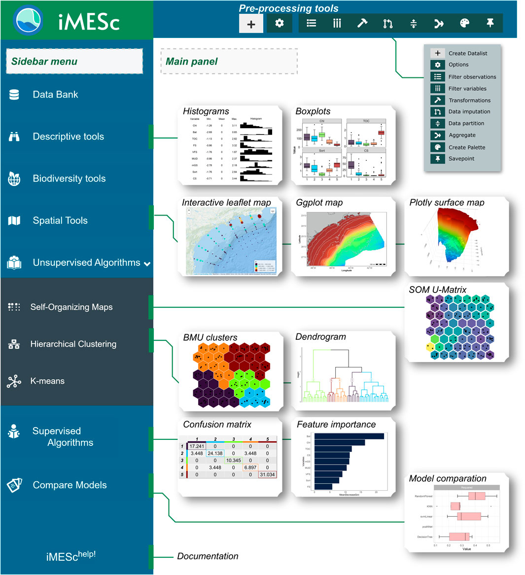
Figure 1. The iMESc app interface, starting with the suite of Pre-processing tools displayed in the top menu, including options for creating a Datalist, filtering observations, filtering variables, applying transformations, imputing missing data, data partitioning, aggregation, and creating savepoints. The Sidebar Menu allows access to other key features, including Data Bank, Descriptive Tools, Biodiversity Tools, Spatial Tools, and both Unsupervised Algorithms (Self-Organizing Maps, Hierarchical Clustering, and K-means) and Supervised Algorithms (such as Random Forest and Gradient Boosting). The Main Panel shows visual outputs such as histograms, boxplots, interactive maps, U-matrix from SOMs, BMU clusters, dendrograms, confusion matrices, feature importance rankings, and model comparison plots.
2.2.1 Pre-processing tools
This section, located in the upper-right corner of the interface, provides quick access to essential tools for preparing datasets. It remains accessible at all times, allowing users to manage and refine their data without needing to navigate away from their current tasks. The pre-processing tools include:
1. Create a Datalist: Allows users to upload and organize datasets into a Datalist format (Supplementary Material SA), supporting attributes like Numeric, Factor, and spatial data. This structure helps maintain consistency and facilitates subsequent analysis.
2. Options: Offers basic functions such as renaming, merging datasets, modifying attribute properties, and managing Datalists.
3. Filter Observations: Provides criteria-based filtering options to remove unwanted or low-quality observations. Users can exclude rows with missing values, zero variance, or specific IDs, ensuring a refined dataset.
4. Filter Variables: Enables users to filter data variables. This includes options to remove variables with low variance, high correlation, or infrequent values, improving data quality.
5. Transformations: Provides a set of transformations for standardizing or normalizing data distributions. Users can apply logarithmic transformations, scaling, Hellinger, or other specialized methods depending on their analysis needs.
6. Data Imputation: Handles missing values by offering multiple imputation techniques, such as k-nearest neighbor (KNN), predictive mean matching, and random forest.
7. Data Partition: Allows users to split data into training and test sets, with options for balanced or random sampling.
8. Aggregate: Computes summary statistics based on a chosen factor. Users can calculate group-level metrics, such as mean or sum.
9. Create Palette: Allows users to create and customize color palettes for visualizations.
10. Savepoint: One of the standout features of iMESc, Savepoint enables users to capture the entire workspace state as an.rds file. This checkpoint feature allows users to pause and resume their work seamlessly without losing progress.
2.2.2 Sidebar menu
Positioned on the left, the sidebar menu acts as the main navigation hub, offering a simple way to access the core modules:
1. Data Bank: Visualize and interact with data tables for different attributes. Includes summaries for saved models.
2. Descriptive Tools: Provides options for visualizations and descriptive statistics like boxplots, correlation plots, Multidimensional Scaling, Principal Component Analysis, and Redundancy Analysis.
3. Spatial Tools: Generates spatial visualizations, offering maps with interpolation methods, circles, pies, rasters, and 3D surfaces.
4. Biodiversity Tools: Computes ecological indices and niche analyses.
5. Unsupervised Algorithms: Includes three modules: Self-Organizing Maps, Hierarchical Clustering and K-Means.
6. Supervised Algorithms: Include 20 supervised algorithms such as Random Forest, Support-Vector Machine, and Gradient Boosting, with validation options like cross-validation.
• Compare Models: Designed to evaluate and contrast the performance of multiple supervised models.
2.2.3 Main Panel
The central area dynamically updates based on the module selected from the sidebar. It features tabbed layouts and interactive widgets for specific analytical tasks, providing relevant controls, outputs, and visualizations.
2.3 Navigation
iMESc streamlines navigation through buttons, dropdown menus and panels. They organize the information to be loaded, effectively guiding users to the next step in their analysis. Particularly, flash buttons are provided when user interactions are required, such as to save the work and run an analysis. This streamlined process also facilitates the transfer of the results between different analysis.
2.4 Dependencies
iMESc integrates several key R packages for both data exploration and machine learning (Table 1). Upon first launch, iMESc checks for necessary libraries and installs them automatically. Although this initial setup might take some time, it ensures smooth operation thereafter. The DT package (Xie et al., 2023) is used for interactive data exploration, enabling users to dynamically filter and sort datasets. For data visualization, ggplot2 (Wickham, 2016) provides flexibility in generating customized plots. The vegan package (Oksanen, 2019) is employed for ordination and biodiversity analysis, supporting the exploration of ecological data.
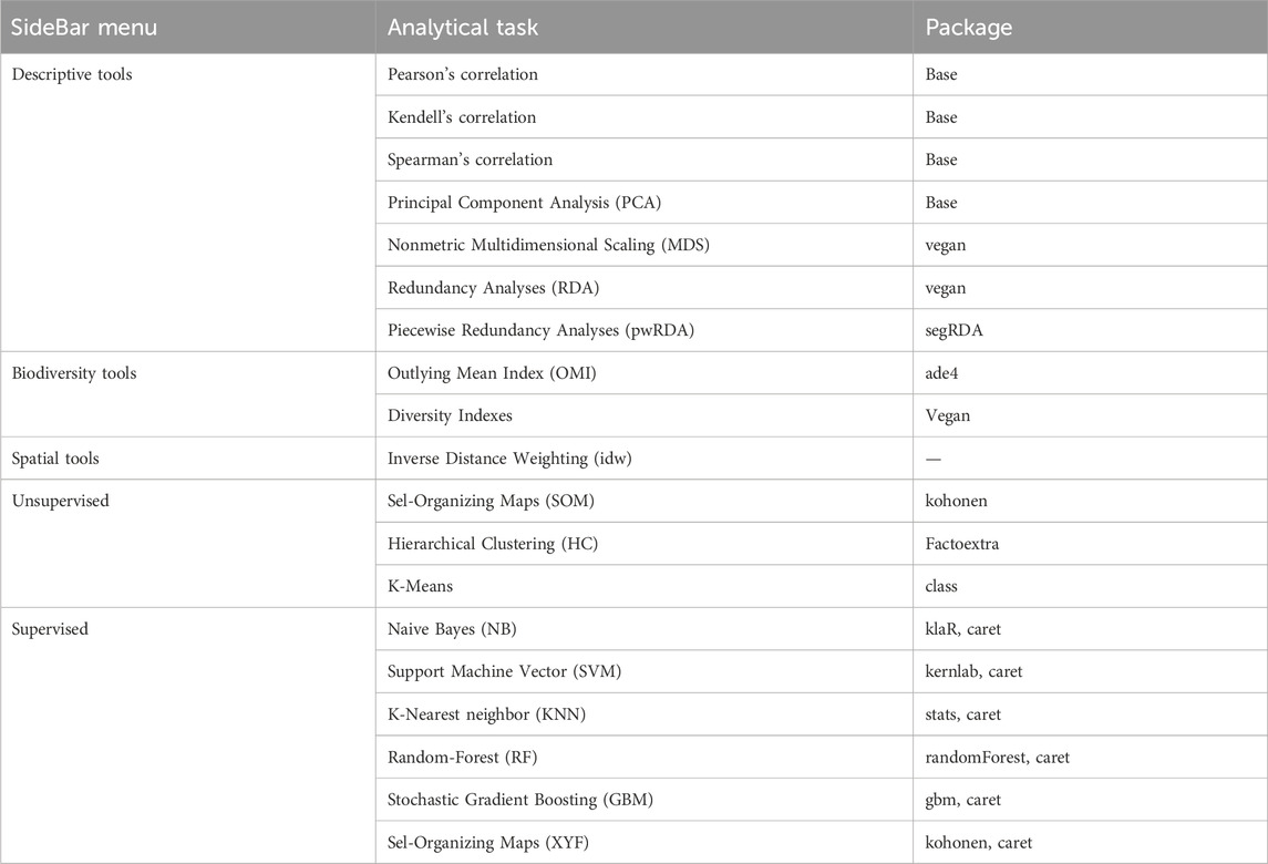
Table 1. A summary of the main analyses used in iMESc, detailing the locations in the sidebar menu, the analytical tasks along with their abbreviations, and corresponding packages.
For unsupervised learning, iMESc utilizes the kohonen package (Wehrens and Kruisselbrink, 2018) for self-organizing maps (SOM), allowing users to cluster and visualize high-dimensional data. Additionally, the factoextra package is used for hierarchical clustering (HC). For supervised learning tasks, iMESc integrates the caret package (Kuhn, 2008), which supports the construction and evaluation of predictive models across 20 algorithms, including Random Forest (Liaw and Wiener, 2020), Support Vector Machines (Karatzoglou et al., 2021), and Gradient Boosting (Ridgeway, 2020). The use of caret ensures consistency in model evaluation across all algorithms, allowing users to compare results in a standardized manner.
For generating maps, iMESc relies on leaflet (Cheng et al., 2019), ggplot2, plotly (Sievert et al., 2021), and sf (Pebesma, 2018). Leaflet enables interactive mapping and dynamic exploration of spatial data with features such as zooming and panning. ggplot2 offers extensive customization for high-quality, static maps that can be tailored for publication purposes. plotly provides 3D visualization capabilities, allowing users to create interactive surface and stack maps. Meanwhile, sf is utilized for handling and manipulating spatial objects, supporting the reading, writing, and transformation of vector data and facilitating spatial analysis and visualization in conjunction with ggplot2.
2.5 Interoperability
At the core of iMESc’s data management is the concept of a Datalist, which can include Numeric-Attribute, Factor-Attribute, and optionally, spatial information. This structure allows users to maintain consistency and organization across different stages of analysis.
iMESc is designed to seamlessly import data and export analysis results in multiple formats, ensuring compatibility with a wide range of external data sources and tools. For data import, iMESc supports common file formats such as CSV, and Excel (.xlsx). During the import process, iMESc validates Datalists to detect potential issues like mismatched rows, ensuring data integrity before processing.
For exporting results, iMESc provides flexible options depending on the type of analysis conducted. Users can export model predictions, processed datasets, and visualizations in various formats, including CSV, Excel, and image files like PNG and PDF. Additionally, spatial data such as rasterized or interpolated maps can be exported as GeoTIFF files, maintaining geographic metadata for further spatial analysis in GIS software.
To enhance the reproducibility of analyses, iMESc offers several key features. During analyses, users can set a seed for model training and evaluation, ensuring consistency in results across different runs. Additionally, iMESc supports saving intermediate results, such as model outputs, in .rds format, for further investigation within R. However, one of iMESc’s standout capabilities is the creation of savepoints, which allow users to capture the entire workspace state as an .rds file. Savepoints act as critical checkpoints, enabling users to easily pause and resume their work without losing progress. When a savepoint is uploaded, iMESc seamlessly restores the workspace to its previous state, allowing for a smooth continuation of the analysis.
2.6 Documentation
iMESc provides immediate assistance through tooltips integrated throughout its interface. As users hover the mouse over or click on a widget, a brief help text is displayed, or a more detailed modal opens, offering clear explanations of the widget functionality. This feature allows users to quickly understand the purpose and usage of various tools, fostering an intuitive and user-friendly experience.
For more in-depth guidance, iMESc offers comprehensive documentation on its help page (https://danilocvieira.github.io/iMESc_help). The documentation covers every aspect of the app, from its structure and panels to the underlying packages. It includes illustrative schemes and tutorial videos that visually guide users through the app’s features, ensuring a thorough understanding of its capabilities.
2.7 Initialization
iMESc can be accessed through RStudio or as a Docker container, depending on the system and user preference.
To run iMESc in RStudio, users need to install R and RStudio. For Windows users, the installation of RTools is required to ensure compatibility with certain packages and functionalities during runtime. Once installed, the following commands should be executed to install and launch iMESc:
Install.packages(“shiny”)
library(“shiny”)
runGitHub('iMESc', 'DaniloCVieira', ref='main')
The first launch may take longer as iMESc automatically installs the required libraries and dependencies. For subsequent launches, the process is faster and can be initiated using:
shiny::runGitHub('iMESc', 'DaniloCVieira', ref = 'main').
Alternatively, iMESc is available as a Docker container, which includes all necessary dependencies. To use this option, users must ensure Docker is installed by following the instructions for their operating system on the Docker website. After Docker is installed, the following commands can be executed to pull the Docker image and start the application.
1. Install Docker by following the instructions for your operating system on the Docker website.
2. Pull the Docker image and start the container by running the following commands:
docker pull vieiradc/imesc docker
run -d -p 3838:3838 vieiradc/imesc
Once the container is running, open your web browser and navigate to http://localhost:3838.
2.8 Workflow examples with nematode data
iMESc provides flexibility for constructing workflows tailored to specific environmental research questions. Each workflow starts with the creation of Datalists, which are structured datasets linked by a common identification column. Detailed guidance on how to format and structure custom Datalists can be found in Supplementary Material SA. iMESc includes two built-in example Datalists: nema_araca, which contains abundance data (expressed as individuals per 10 cm2) from 141 samples of free-living marine nematodes across 194 species, and envi_araca, containing 9 environmental variables for the same samples. Both Datalists include a Factor-Attribute with columns for season (Spring, Summer, Autumn, Winter), site (1–37), and depth.area—an a priori classification grouping depth zones into specific ranges: intertidal (0.06–0.80 m), shallow (−0.18–0.44 m), medium (−7.68–0.70 m), and deep (−23.02–9.08 m). Additionally, a Coords-Attribute provides geographic coordinates for each of the 37 sites across all seasons. Details about the sampling methodology and dataset formation can be found in Corte et al. (2017).
Here we explore four workflows covering different analytical tools and varying degrees of complexity. All of them share the same pre-processing steps that used the Pre-Processing Tools to prepare datasets: the Transformation Tool was applied to perform a Hellinger transformation on the nematode data (saved as nema_araca_hellinguer) and this same tool was used to scale and center the environmental variables (saved as envi_araca_scaled) for subsequent analyses (Figure 2). The “savepoint” with results from all workflows can be found in https://github.com/DaniloCVieira/iMESc_savepoints/tree/main/iMESc%20%E2%80%93%20A%20interactive%20machine%20learning%20app%20for%20environmental%20sciences.

Figure 2. Diagram of data preprocessing in iMESc: The first step involves selecting the example Datalists (nema_araca, envi_araca) using the “example” option. In the second step, users can apply a Hellinger transformation to nema_araca and scale/center variables for envi_araca, resulting in new datasets (nema_araca_hellinger, envi_araca_scaled) for subsequent analysis. Green lines indicate the flow between steps. Triangular dropdowns represent user selections (e.g., choosing input Datalists or transformation types), blue disk icons denote save buttons, and narrow blue vertical bars show fields where users can enter text manually.
2.8.1 Workflow 1: RDA
The first analytical workflow runs in the Descriptive Tools module, using Redundancy Analysis (RDA) to model the nematode species data as a function of the enviornmental variables (Figure 3A). The envi_araca_scaled data was used as predictors, while nema_araca_hellinguer served as the response. iMESc generates an RDA biplot with ggplot2, visually representing the distribution of nematode species in relation to environmental gradients. Users can access the factors within the Factor-Attribute associated with the respective Datalist to color the dots. This tool allows the visual differentiation of the dots based on categorical variables. The RDA returns a R2 value that quantifies the proportion of variance in the species data explained by the environmental variables, a p-value and the importance of each canonical axis to the full model.
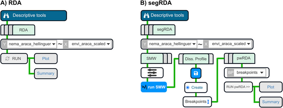
Figure 3. Diagrams of two workflows in the Descriptive Tools module. In both workflows, envi_araca_scaled was selected as the predictor Datalist (X) and nema_araca_hellinger as the response Datalist (Y). User selections are represented by triangular dropdowns (e.g., choosing X and Y). Light green rectangles denote tab panels, blue disk icons indicate save buttons, and narrow blue vertical bars show fields for manual text input. (A) Redundancy Analysis (RDA) workflow. (B) Segmented RDA (segRDA) workflow, which included the SMW (Split Moving Window) analysis to generate a dissimilarity profile and identify breakpoints (BP). These breakpoints were saved and then used in the piecewise RDA (pwRDA) analysis. The sliders icon represented parameter settings for the SMW analysis (e.g., window size and dissimilarity method).
2.8.2 Workflow 2: segRDA
This second workflow, also running in the Descriptive Tools module, applies the segRDA framework (Vieira et al., 2019) to perform Piecewise Redundancy Analysis (pwRDA) (Figure 3B). As in Workflow 1, the envi_araca_scaled data served as predictors, and nema_araca_hellinguer as the response. Samples were first ordered based on the first axis of the RDA, and dissimilarity profiles were computed across multiple window sizes (10, 26, 40, 56, 70) to identify significant ecological breakpoints. With these breakpoints, pwRDA was applied to model species-environment relationships. This method allows the detection of non-continuous linear responses when multiple discontinuous communities are present in the data set (Vieira et al., 2019). Similar to traditional RDA, pwRDA returns a biplot, an R2 value that quantifies the proportion of variance explained by environmental gradients, the importance of each canonical axis and a p-value, which compares its performance against the original RDA model.
2.8.3 Workflow 3: SuperSOM
The third workflow is performed in the Unsupervised Algorithms module, using a two-layer Self-Organizing Map (SOM) to simultaneously cluster both environmental and nematode species data into neurons (Figure 4). Although traditionally used as an unsupervised technique, the inclusion of environmental variables as input effectively transforms the SOM into a supervised learning method, enabling the prediction of nematode community patterns based on the environmental conditions.
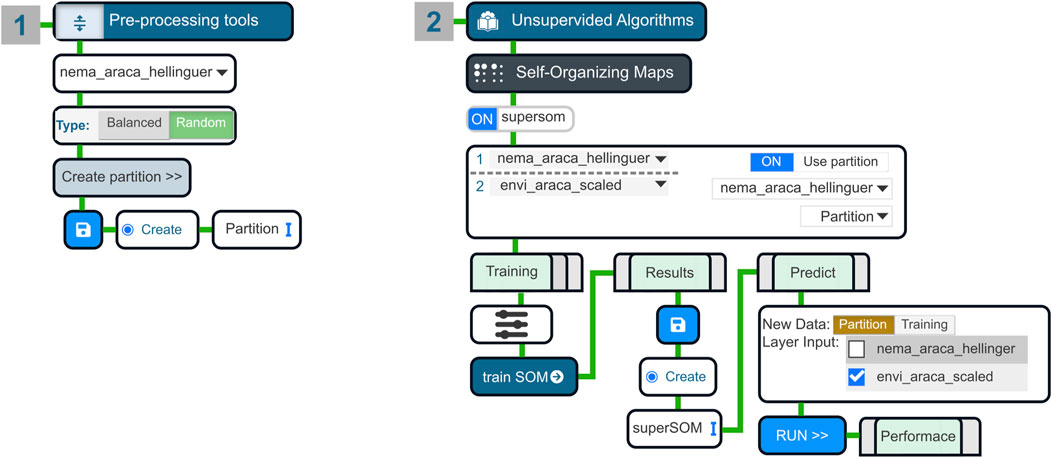
Figure 4. Diagram of the superSOM workflow. Green lines indicate the flow of processes between steps. User selections are represented by triangular dropdowns (e.g., choosing X and Y). Light green rectangles denote tab panels, blue disk icons represent save buttons, and narrow blue vertical bars indicate fields for manual text input. Step 1 involved data preprocessing, where the nema_araca_hellinger Datalist was selected, and a random partition was created. In Step 2, the superSOM model was configured in the Self-Organizing Maps (SOM) module, using both nema_araca_hellinger and envi_araca_scaled as layer inputs. After setting the training parameters (slider icon), the model was trained and saved. The performance of predictions on nema_araca_hellinger was evaluated for both training and test data, using envi_araca_scaled as the input layer.
The workflow begins with the “Create partition” tool in the Pre-Processing Tools to generate a random partition in the nema_araca_hellinguer dataset. Here the training and testing sets were separated into a one-to-five ratio. In the SOM module, nema_araca_hellinguer and envi_araca_scaled datasets are set as input layers with equal weights, applying Euclidean distance to compute dissimilarities across both layers. After setting the input layers, the previously created partition is selected. Particularly for this analysis, a grid size of 6 × 5 was chosen to avoid empty neurons while capturing sufficient detail in the network. For unsupervised one-layer SOMs we recommend the use of the default settings which can end up with empty neurons evaluation (Fonseca and Vieira, 2023). To ensure reproducibility, the seed 42 was applied during the SOM configuration.
The trained SOM model was saved (iMESc stores it within the Datalist used in the first layer (nema_araca_hellinger) and results were visualized through four codebook plots: the counts (number of observations in each neuron), the Best Matching Unit (BMU) plot and the Codebooks Pie Charts from the nematodes and environmental data. The BMU plot displays the sample distribution across the SOM grid, with options for users to color the sample points by factor from the Factor-Attribute associated with the Datalist. The Codebook Pie Chart highlights the contribution of each variable (species or environmental depending on the layer) to the classification of the samples to the corresponding neuron, based on the codebook weights. Additionally, an R2 value was computed by contrasting the predicted values from the SOM nema_araca_hellinger model with the observed nematode data (nema_araca_hellinger training data). The R2 was performed for the training and test part of the datasets.
2.8.4 Workflow 4: hybrid model
The fourth workflow is a hybrid approach that combines unsupervised and supervised methods to model nematode species using environmental predictors (Figure 5). First, the SOM analysis from the unsupervised module was used to cluster the nema_araca_hellinguer data into one-layer of neurons. The trained SOM model was saved within the nema_araca_hellinger Datalist, allowing it to be accessed in subsequent steps (Figure 5-1).
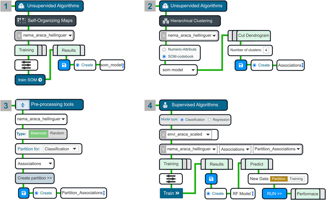
Figure 5. Diagram of the Hybrid Model workflow. Green lines indicate the flow of processes between steps. User selections are represented by triangular dropdowns (e.g., choosing X and Y). Light green rectangles denote tab panels, blue disk icons represent save buttons, and narrow blue vertical bars indicate fields for manual text input. Step 1: A one-layer Self-Organizing Map (SOM) was trained using nema_araca_hellinger. Step 2: Hierarchical clustering was applied to the SOM codebook, with an option to select the number of clusters, and the resulting clusters were saved as “Associations.” Step 3: In the Pre-processing tools, the “Create Partition” function for classification models was used to create a balanced partition (training and test) based on “Associations” and saved as “Partition_Associations.” Step 4: In the Supervised Algorithms module, the model type was set to Classification, envi_araca_scaled was selected as the predictor (X), nema_araca_hellinger as the response (Y), and the “Partition_Associations” was used to separate training and test sets. After setting training parameters (slider icon), the model was trained, saved, and results were explored, with predictions run on both training and test data to assess performance.
In the HC module, the saved SOM model within the nema_araca_hellinger Datalist was accessed to perform hierarchical clustering of the codebook using the Ward.D2 method (Murtagh and Legendre, 2014). By inspecting the elbow plot and performing a moving split window technique, this step divided the SOM codebook into four distinct clusters of neurons (Figure 5-2). In the current context, each cluster represents a taxonomic association. A dendrogram plot was generated to illustrate the hierarchical relationships among clusters, while the Codebook Clusters plot was used to visualize the clustering structure of the network. Once the clusters are saved, an additional column is created in the factor attribute of the original Datalist (nema_araca_hellinguer).
The next step consisted in generating a balanced partition of the data among the clusters for training and testing. This step was conducted in the Pre-Processing Tools, specifically the “Create partition” tool (Figure 5-3). This ensured that both the training and testing sets had a proportional representation of samples from each cluster. The Supervised Algorithms module was then used to apply the Random Forest algorithm (RF), with envi_araca_scaled dataset serving as predictors of the clusters identified by the HC (Figure 5-4). The RF model was configured with 500 trees, 5-fold cross-validation, 5 repetitions, and a seed value of 42 for reproducibility.
3 Workflow results with nematode data
3.1 RDA
The RDA analysis revealed that the environmental gradient significantly structured the nematode communities. In this model, the environmental data explained 30.7% of the variation in nematode species distribution (Figure 6A). When grouping the samples according to its depth (an a priori classification), the intertidal and shallow zones were associated with Very Fine Sand, Fine Sand, and the Sorting Coefficient. Deeper zone samples were more strongly related to Chlorophyll and Total Organic Carbon.

Figure 6. Results from the Descriptive Workflows. (A) Biplot from Redundancy Analysis (RDA): Environmental variables are represented as blue vectors, and sample points are colored according to four depth zones: intertidal, shallow, medium, and deep. Red crosses represent species data (response variables). (B) Dissimilarity profile from the Split-Moving Window (SMW) Analysis: Points represent the z-score dissimilarity across ordered samples, with significant z-scores shown in black and significant breakpoints indicated in red. (C) Biplot from the Piecewise Redundancy Analysis (pwRDA): Similar to the RDA, environmental variables are shown as blue vectors, and sample points are colored by depth zone. Red crosses represent species data. Variable abbreviations: Bat - bathymetry, Chl - chlorophyll, CS - coarse sand, Mud - mud content, TOC - total organic carbon, mGS - mean grain size, VFS - very fine sand, Sort - sorting, FS - fine sand.
3.2 pwRDA
In the piecewise RDA (pwRDA) model, the environmental data explained 53.6% of the variance in nematodes composition. This method recognized four breakpoints (Figure 6B), pointing for a non-continuous species-environment relationships. While deeper and medium-depth zones were more distinctly clustered, with stronger influences from Coarse Sand and Mean Grain Size, shallower stations were associated, for instance, with Fine Sand, Very Fine Sand and Chlorophyll A (Figure 6C). In comparison to the RDA, this model improved the explained variance by 23%.
3.3 SuperSOM
Modeling the nematode species composition using the SuperSOM returned a R2 of 0.60 for the training data and 0.291 for the test data. This reduction in R2 indicates a decrease in model performance when applied to unseen data. Most of the neurons grouped more than one station from the same depth-zone (Figure 7A). Test samples were spread across the neurons (Figure 7B), indicating that the model had the potential to capture the spatial patterns across depth zones. The left region of the BMU map primarily consisted of intermediate and deep stations, which were characterized by higher concentrations of MUD and TOC (Figure 7C). By contrast, the right region represented shallow stations, where very fine sand (VFS) and fine sand (FS) were predominant (Figure 7C). Regarding species distribution, the left region was dominated by Terschellingia sp5, while the right region was characterized by Dorylaimopsis_1 and Odontophora_1 as characteristic species (Figure 7D).
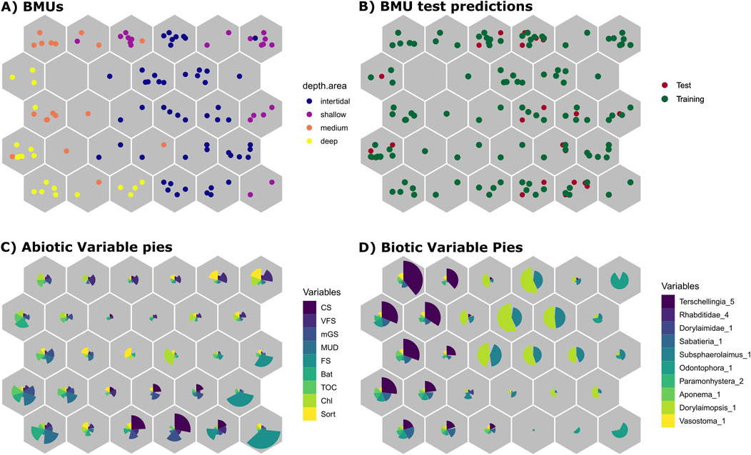
Figure 7. Self-Organizing Map (SOM) visualizations. (A) Codebook Best Matching Unit (BMU) plot showing the distribution of samples across the SOM grid, with observations colored according to depth areas: intertidal, shallow, medium, and deep. (B) BMU plot with test predictions, where points are colored to differentiate between test and training datasets. (C, D) Codebook Pie charts show the 10 most important abiotic (C) and biotic (D) variables from the SOM, indicating the relative contributions to the classification of each hexagon (neuron).
3.4 Hybrid model
The hybrid model (Figures 8A, B) grouped the neurons from the unsupervised phase into four distinct clusters. The distribution of the clusters remained consistent across seasons, with clusters 1 and 2 predominantly occupying shallow regions, while clusters 3 and 4 were associated with deeper areas (Figure 8C). Random Forest predictions achieved an accuracy of 83.47% for the training phase and of 80.77% for test (Figure 8D). The model showed the highest prediction accuracy for clusters 1 and 3, while the greatest misclassifications occurred for cluster 4 during both training and testing phases. The feature importance demonstrated that Bathymetry, Chlorophyll, and Coarse Sand were the most important variables driving the cluster predictions (Figure 8E). Regarding the depth zones, deep and medium stations were mostly grouped in cluster 1, shallow stations were predominantly in cluster 2, while intertidal samples were separated in two clusters, three and four (Figure 8B). Cluster 3 occurred next to the coastline, while cluster 4 covered most of the intertidal zone.

Figure 8. Graphical outputs of the Hybrid model. (A) Dendrogram showing hierarchical clustering (HC) into four groups of the SOM neurons. (B) Codebook Clusters plot, illustrating the clustering structure on the SOM grid with different background colors representing the four clusters and and colored points indicating sample depth zones (intertidal, shallow, medium, and deep). (C) Spatial Distribution of the clusters across four seasons (spring, summer, autumn, and winter). Each map shows the spatial distribution of samples by cluster. (D) Confusion Matrices displaying the accuracy of the Random Forest model for both training and test datasets, with class errors per group. (E) Feature Importance plot showing the importance of the environmental variables in predicting nematode species associations: Bathymetry (Bat), Chlorophyll (Chl), Coarse Sand (CS), Mud, Total Organic Carbon (TOC), Mean Grain Size (mGS), Very Fine Sand (VFS), Sorting (Sort) and Fine Sand (FS). Number inside the box represents the average depth distribution of the variable after considering all the trees.
4 Discussion
4.1 Adaptive workflows in iMESc boost efficiency
One of the most significant contributions of iMESc to environmental data analysis is its ability to organize and streamline complex, non-linear workflows. iMESc is not just a collection of tools, but a comprehensive solution that facilitates seamless transitions between different stages of analysis, fostering a more efficient and holistic approach to environmental data analysis. Environmental science often requires a flexible approach to data analysis due to the inherent variability of research questions and ecological data. iMESc addresses this by allowing users to construct customized workflows that can incorporate iterative refinement, conditional branching, and looping mechanisms (Figure 9). These characteristics are critical for enabling adaptive analysis, where insights gained during the process inform subsequent steps. For instance, conditional branching allows users to explore different analytical paths based on specific criteria, while the looping mechanism ensures repeatability, refining individual stages as needed.
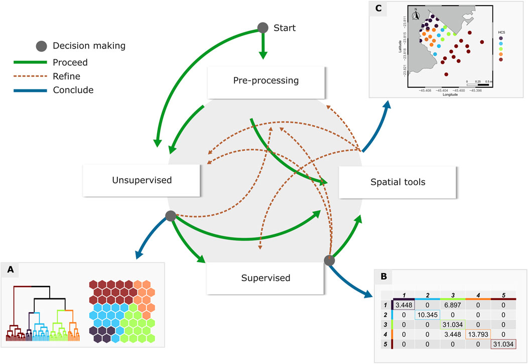
Figure 9. Scheme Illustrating the versality of analytical workflows in iMESc. Example of sequential stages in the analytical process with alternative progress paths (green arrows), refinements (dashed brown arrows), or conclusion paths (blue arrows) with graphical outputs: (A) dendrogram and Self-Organizing Map; (B) confusion matrix; (C) Spatialization.
In environmental science, the need for combining multiple types of analyses—such as unsupervised clustering, supervised learning, and spatial mapping—is critical for fully understanding the complexity of ecological systems evaluation (Fonseca and Vieira, 2023). iMESc’s architecture enables this integration seamlessly, allowing users to move from one analysis module to another without having to export, reformat, or manually transfer data between different platforms. By eliminating these technical hurdles, iMESc makes advanced machine learning methods more accessible and enables researchers to focus on refining their analyses rather than programing and managing data logistics. However, a solid understanding of the underlying statistical techniques remains essential to ensure reliable and meaningful results.
iMESc also provides robust pre-processing capabilities that enhance data preparation. The platform supports a wide range of pre-processing techniques, typically applied in environmental studies, including handling missing data, applying transformations, and partitioning data for training and testing (Fonseca and Vieira, 2023). Moreover, the ability to store and manage data through the “Datalist” system enables users to organize their data efficiently, facilitating the use of multiple datasets across different stages of the analysis.
The modular design of iMESc enhances the construction of workflows and promotes flexibility in adapting to future needs, facilitating the prevention of programing errors and conflicts (Chen and Nof, 2023). iMESc was primarily designed to address the specific needs of oceanographers and environmental scientists (Brito de Jesus et al., 2023; Fonseca and Vieira, 2023; Gallucci et al., 2023), focused on workflows applicable to these fields. However, the platform is structured in a way that allows new modules or algorithms to be added without significant restructuring, making it an adaptable tool for evolving research needs. Furthermore, compatibility with Docker makes it the best solution in terms of scalability, as it could be easily deployed on different operating systems. This flexibility ensures the long life of iMESc, the continuous support to a broad range of environmental research questions as new analytical methods and data sources emerge.
4.2 Real-time modeling and customization refine interpretation
A standout feature of iMESc is its real-time interactivity, allowing users to receive immediate feedback as they experiment with different models and parameters. Interactive visualizations allow multiple perspectives and enable quick identification of relationships and trends by letting users adjust parameters and instantly see the effects (Khedr and Hilal, 2021). This dynamic interactivity streamlines the research process, enabling rapid hypothesis testing and model refinement without the need for extensive re-running of analyses. This is particularly advantageous in environmental research, where iterative and feedback adjustments to models are often necessary to capture complex ecological dynamics (An et al., 2021). We share the opinion that the interpretation of complex machine learning models through metrics, tables and figures is an important step in building confidence in a model, or in a specific prediction from a model, to foster the understanding of the research problem (Lucas, 2020).
iMESc’s visual outputs also contribute to its user-centric design. The platform supports a high degree of customization, leveraging ggplot2 to allow users to tailor every aspect of their visualizations, from axis labels and color schemes to finer plot aesthetics. This is crucial in environmental science, where clear, publication-ready figures are necessary to convey intricate patterns in large datasets (Aigouy and Mirouse, 2013). Moreover, iMESc supports multiple export formats (e.g., png and pdf) with adaptable resolutions, ensuring flexibility in how results are shared and disseminated. The visual tools provided by iMESc, including sophisticated plots, play an essential role in translating complex data into interpretable results, guiding researchers in drawing meaningful ecological conclusions.
4.3 Reproducibility in iMESc strengthens research continuity
Beyond these technical advantages, iMESc places a strong emphasis on reproducibility, a cornerstone of the FAIR principles of modern scientific research (Bailo et al., 2022; Barker et al., 2022). The ability to create “savepoints” at different stages of the analysis allows users to preserve their workflows and return to them at any time, ensuring that their work can be revisited or shared with collaborators without loss of context or data. This focus on reproducibility is essential in environmental research, where projects often involve long-term data collection and collaboration across multiple teams. By documenting every step of the analysis and providing the ability to replicate it easily, iMESc helps safeguard the transparency and integrity of scientific findings. Furthermore, this feature encourages collaboration, as entire workflows can be shared with other researchers, promoting consistency across studies (Stoudt et al., 2021). The “savepoints” can be shared by journal repositories (e.g., Brito de Jesus et al., 2023) or in the github (https://github.com/DaniloCVieira/iMESc_savepoints).
4.4 Multi-model approaches in iMESc deepen insights
The integration of traditional exploratory methods (e.g., RDA, pwRDA) with advanced machine learning approaches (e.g., SOM, RF) in iMESc demonstrates the platform’s versatility in addressing a broad range of research questions and analytical needs - essential for capturing the inherent complexity of ecological data (Gilbert et al., 2024).
While both RDA and pwRDA help establish species-environment relationships, our analysis suggests that pwRDA may better capture the discontinuous nature of ecological shifts present in our dataset. The presence of ecological breakpoints is a consequence of non-linear responses of species distributions to environmental gradients (Fujita et al., 2023; Pélissié et al., 2024). By accommodating these abrupt transitions, pwRDA provides a nuanced perspective on ecosystem dynamics that RDA, with its assumption of linear continuity, might only partially represent (Vieira et al., 2019) iMESc facilitates the comparison between RDA and pwRDA models, offering a clear advantage in determining which approach best aligns with the structure of the data.
Supervised machine learning methods, such as SuperSOM, enhance analytical power by accommodating non-linear patterns beyond the linear framework. SuperSOM enables flexible, pattern-based exploration that adapts to complex, multidimensional relationships without predefined assumptions (Giraudel and Lek, 2001). By clustering species and environmental variables into neurons, SuperSOM reveals community structures that traditional methods might overlook. Additionally, SuperSOM introduces a predictive capacity, allowing researchers to assess model generalization through performance metrics (e.g., R2) across training and test datasets. Our results indicated moderate generalization when using environmental variables to predict nematode composition. This suggests that while SuperSOM effectively captures essential ecological patterns, further refinement is needed to enhance its predictive robustness.
Extending beyond individual models, iMESc’s integration of multiple machine learning approaches into hybrid models enhances analytical power, enabling researchers to delve deeper into emergent patterns. In the hybrid model example presented, SOM first organizes data based on multidimensional relationships among taxa. HC then refines these groupings, forming ecologically coherent clusters that improve the data structure for the RF model (Koudenoukpo et al., 2021; Santos et al., 2021; Fonseca and Vieira, 2023). This approach strengthens predictive power by isolating relevant patterns, allowing for more accurate and interpretable predictions that align with the complexity of ecological systems.
iMESc’s integration of both exploratory and predictive techniques highlights the complementary nature of traditional and machine learning approaches. Exploratory methods, like RDA and pwRDA, offer valuable insights into species-environment relationships by formalizing our understanding of ecological processes through model-based inferences. These methods enable researchers to draw statistically supported conclusions about the relevance of environmental gradients and community structures, which is essential for hypothesis-driven studies. It is important to keep in mind that in RDA and pwRDA, the R2 represents the extent to which environmental variables account for variance in species composition within a linear framework and do not indicate predictive accuracy on new data. On the other hand, machine learning methods, such as SuperSOM and RF, prioritize prediction and are particularly suited for data-intensive applications where the number of variables often exceeds the sample size (Bzdok et al., 2018). ML methods yield predictive R2 values that assess the model’s ability to generalize patterns to new data, thus serving as a reliable measure for forecasting. By incorporating both approaches, iMESc supports a comprehensive framework, where exploratory models deepen our understanding of system structure, while ML algorithms capture predictive patterns that inform future research and decision-making. This dual capability underscores the value of integrating both exploratory and machine learning techniques in ecological studies, as they offer complementary perspectives on ecosystem complexity.
Availability as a docker image which makes it the best solution in terms of scalability, as it could be easily deployed on different operating systems.
5 Conclusion
iMESc was developed to empower environmental researchers to apply ML methods though a user-friendly interface, eliminating the need for programming knowledge. With iMESc researchers gain the ability to apply a range of ML algorithms in a variety of scientific research questions. By combining real-time interactivity with customizable visualization options, iMESc offers a distinct advantage over traditional static machine learning tools, empowering researchers to explore their data in a more flexible, iterative manner. The platform was designed to facilitate data and analysis sharing, ensuring collaboration and reproducibility of research findings. iMESc enables ecologists and environmental researchers to move from the traditional hypothesis testing approach to a predictive one, a fundamental step for implementing monitoring programs, supporting informed management decision, and, ultimately, conserving natural ecosystems.
Data availability statement
Original datasets are available in a publicly accessible repository: https://doi.org/10.6084/m9.figshare.28254569.
Ethics statement
The manuscript presents research on animals that do not require ethical approval for their study.
Author contributions
DV: Conceptualization, Data curation, Formal Analysis, Investigation, Methodology, Resources, Software, Supervision, Validation, Visualization, Writing–original draft, Writing–review and editing. FP: Conceptualization, Methodology, Validation, Visualization, Writing–review and editing. LY: Formal Analysis, Validation, Visualization, Writing–review and editing. GF: Conceptualization, Data curation, Formal Analysis, Funding acquisition, Investigation, Methodology, Project administration, Supervision, Validation, Visualization, Writing–review and editing.
Funding
The author(s) declare that financial support was received for the research, authorship, and/or publication of this article. BRAZILIAN National Petroleum Agency - ANP (PD&I). São Paulo Research Foundation (FAPESP 2011/50317-5). National Council for Scientific and Technological Development (CNPQ 306780/2022-4.)
Acknowledgments
We thank PETROBRAS and BRAZILIAN National Petroleum Agency - ANP (grant and research funds under resolution ANP PD&I) The authors acknowledge all the feedback received from Santos-Project working group on preliminary versions of the app. The available data has been generated under the project FAPESP 2011/50317-5. Gustavo Fonseca acknowledges the support of CNPQ under grant number 306780/2022-4. The authors acknowledge all the feedback received from Santos-Project working group on preliminary versions of the app.
Conflict of interest
The authors declare that the research was conducted in the absence of any commercial or financial relationships that could be construed as a potential conflict of interest.
Generative AI statement
The author(s) declare that no Generative AI was used in the creation of this manuscript.
Publisher’s note
All claims expressed in this article are solely those of the authors and do not necessarily represent those of their affiliated organizations, or those of the publisher, the editors and the reviewers. Any product that may be evaluated in this article, or claim that may be made by its manufacturer, is not guaranteed or endorsed by the publisher.
Supplementary material
The Supplementary Material for this article can be found online at: https://www.frontiersin.org/articles/10.3389/fenvs.2025.1533292/full#supplementary-material
References
Abid, A., Abdalla, A., Abid, A., Khan, D., Alfozan, A., and Zou, J. (2020). An online platform for interactive feedback in biomedical machine learning. Nat. Mach. Intell. 2, 86–88. doi:10.1038/s42256-020-0147-8
Aigouy, B., and Mirouse, V. (2013). ScientiFig: a tool to build publication-ready scientific figures. Nat. Methods 10, 1048. doi:10.1038/nmeth.2692
An, L., Grimm, V., Sullivan, A., Turner II, B. L., Malleson, N., Heppenstall, A., et al. (2021). Challenges, tasks, and opportunities in modeling agent-based complex systems. Ecol. Modell. 457, 109685. doi:10.1016/j.ecolmodel.2021.109685
Bailo, D., Jeffery, K. G., Atakan, K., Trani, L., Paciello, R., Vinciarelli, V., et al. (2022). Data integration and FAIR data management in solid earth science. Ann. Geophys. 65, DM210. doi:10.4401/ag-8742
Barker, M., Chue Hong, N. P., Katz, D. S., Lamprecht, A.-L., Martinez-Ortiz, C., Psomopoulos, F., et al. (2022). Introducing the FAIR Principles for research software. Sci. Data 9, 622. doi:10.1038/s41597-022-01710-x
Bolduc, B., Zablocki, O., Guo, J., Zayed, A. A., Vik, D., Dehal, P., et al. (2021). iVirus 2.0: cyberinfrastructure-supported tools and data to power DNA virus ecology. ISME Commun. 1, 77. doi:10.1038/s43705-021-00083-3
Brito de Jesus, S., Vieira, D., Gheller, P., Cunha, B. P., Gallucci, F., and Fonseca, G. (2023). Machine learning algorithms accurately identify free-living marine nematode species. PeerJ 11, e16216. doi:10.7717/peerj.16216
Bzdok, D., Altman, N., and Krzywinski, M. (2018). Points of significance: statistics versus machine learning. Nat. Methods 15, 233–234. doi:10.1038/nmeth.4642
Chang, W., Cheng, J., Allaire, J. J., Sievert, C., Schloerke, B., Xie, Y., et al. (2022). Shiny: web application framework for R.
Chen, X. W., and Nof, S. Y. (2023). Automating prognostics and prevention of errors, conflicts, and disruptions. Conflicts, Disruptions, 509–531. doi:10.1007/978-3-030-96729-1_22
Cheng, J., Karambelkar, B., Xie, Y., Wickham, H., Russell, K., Johnson, K., et al. (2019). Package ‘leaflet.’ R package version 2.
Corte, G. N., Checon, H. H., Fonseca, G., Vieira, D. C., Gallucci, F., Domenico, M. D., et al. (2017). Cross-taxon congruence in benthic communities: searching for surrogates in marine sediments. Ecol. Indic. 78, 173–182. doi:10.1016/j.ecolind.2017.03.031
Fonseca, G., and Vieira, D. C. (2023). Overcoming the challenges of data integration in ecosystem studies with machine learning workflows: an example from the Santos project. Ocean Coast. Res. 71. doi:10.1590/2675-2824071.22044gf
Fujita, H., Ushio, M., Suzuki, K., Abe, M. S., Yamamichi, M., Iwayama, K., et al. (2023). Alternative stable states, nonlinear behavior, and predictability of microbiome dynamics. Microbiome 11, 63. doi:10.1186/s40168-023-01474-5
Gallucci, F., Corbisier, T. N., Gheller, P., Brito, S., Vieira, D. C., Fonseca, G., et al. (2023). Predicting large-scale spatial patterns of marine meiofauna: implications for environmental monitoring. Ocean Coast. Res. 71. doi:10.1590/2675-2824071.22070fg
Gilbert, N. A., Amaral, B. R., Smith, O. M., Williams, P. J., Ceyzyk, S., Ayebare, S., et al. (2024). A century of statistical Ecology. Ecology 105, e4283. doi:10.1002/ecy.4283
Giraudel, J. L., and Lek, S. (2001). A comparison of self-organizing map algorithm and some conventional statistical methods for ecological community ordination. Ecol. Modell. 146, 329–339. doi:10.1016/S0304-3800(01)00324-6
Heil, B. J., Hoffman, M. M., Markowetz, F., Lee, S.-I., Greene, C. S., and Hicks, S. C. (2021). Reproducibility standards for machine learning in the life sciences. Nat. Methods 18, 1132–1135. doi:10.1038/s41592-021-01256-7
Hu, J., Stefanov, S., Song, Y., Omee, S. S., Louis, S. Y., Siriwardane, E. M. D., et al. (2022). MaterialsAtlas.org: a materials informatics web app platform for materials discovery and survey of state-of-the-art. NPJ Comput. Mater 8, 65–12. doi:10.1038/s41524-022-00750-6
Karatzoglou, A., Smola, A., Hornik, K., Maniscalco, M. A., and Teo, C. H. (2021). Kernlab: kernel-based machine learning lab. Available at: https://cran.r-project.org/package=kernlab.
Khedr, A., and Hilal, S. (2021). “Interactive visualization for statistical modelling through a shiny app in R,” in 2021 international conference on data analytics for business and industry, ICDABI 2021, 332–337. doi:10.1109/ICDABI53623.2021.9655841
Kohonen, T. (2001). Self-organizing maps. Berlin, Heidelberg: Springer Berlin Heidelberg. doi:10.1007/978-3-642-56927-2
Koudenoukpo, Z. C., Odountan, O. H., Agboho, P. A., Dalu, T., Van Bocxlaer, B., Janssens de Bistoven, L., et al. (2021). Using self–organizing maps and machine learning models to assess mollusc community structure in relation to physicochemical variables in a West Africa river–estuary system. Ecol. Indic. 126, 107706. doi:10.1016/j.ecolind.2021.107706
Kuhn, M. (2008). Building predictive models in R using the caret package. J. Stat. Softw. 28. doi:10.18637/jss.v028.i05
Legendre, P., and Legendre, L. (2012). “Canonical analysis,” , 625–710. doi:10.1016/B978-0-444-53868-0.50011-3
Liaw, A., and Wiener, M. (2020). randomForest: breiman and cutler’s random forests for classification and regression. Available at: https://cran.r-project.org/package=randomForest.
Lucas, T. C. D. (2020). A translucent box: interpretable machine learning in ecology. Ecol. Monogr. 90. doi:10.1002/ecm.1422
Moreira, D. L., Dalto, A. G., Figueiredo, A. G., Valerio, A. M., Detoni, A. M. S., Bonecker, A. C. T., et al. (2023). Multidisciplinary scientific cruises for environmental characterization in the Santos basin – methods and sampling design. Ocean Coast. Res. 71. doi:10.1590/2675-2824071.22072dlm
Murtagh, F., and Legendre, P. (2014). Ward’s hierarchical agglomerative clustering method: which algorithms implement ward’s criterion? J. Classif. 31, 274–295. doi:10.1007/s00357-014-9161-z
Pebesma, E. (2018). Simple features for R: standardized support for spatial vector data. R. J. 10, 439–446. doi:10.32614/RJ-2018-009
Pélissié, M., Devictor, V., and Dakos, V. (2024). A systematic approach for detecting abrupt shifts in ecological timeseries. Biol. Conserv. 290, 110429. doi:10.1016/j.biocon.2023.110429
Ridgeway, G. (2020). Gbm: generalized boosted regression models. Available at: https://cran.r-project.org/package=gbm.
R Core Team (2023). R: A language and environment for statistical computing. Available at: https://www.r-project.org/.
Santos, L. A., Ferreira, K., Picoli, M., Camara, G., Zurita-Milla, R., and Augustijn, E. W. (2021). Identifying spatiotemporal patterns in land use and cover samples from satellite image time series. Remote Sens. (Basel) 13, 974–1021. doi:10.3390/rs13050974
Sievert, C., Parmer, C., Hocking, T., Chamberlain, S., Ram, K., Corvellec, M., et al. (2021). Package ‘plotly. Vienna: ’ R Foundation for Statistical Computing.
Stoudt, S., Vásquez, V. N., and Martinez, C. C. (2021). Principles for data analysis workflows. PLoS Comput. Biol. 17, e1008770. doi:10.1371/journal.pcbi.1008770
Tahmasebi, P., Kamrava, S., Bai, T., and Sahimi, M. (2020). Machine learning in geo- and environmental sciences: from small to large scale. Adv. Water Resour. 142, 103619. doi:10.1016/j.advwatres.2020.103619
Vieira, D. C., Brustolin, M. C., Ferreira, F. C., and Fonseca, G. (2019). segRDA: an r package for performing piecewise redundancy analysis. Methods Ecol. Evol. 10, 2189–2194. doi:10.1111/2041-210X.13300
Walsh, I., Fishman, D., Garcia-Gasulla, D., Titma, T., Pollastri, G., Capriotti, E., et al. (2021). DOME: recommendations for supervised machine learning validation in biology. Nat. Methods 18, 1122–1127. doi:10.1038/s41592-021-01205-4
Wehrens, R., and Kruisselbrink, J. (2018). Flexible self-organizing maps in kohonen 3.0. J. Stat. Softw. 87. doi:10.18637/jss.v087.i07
Wickham, H. (2016). ggplot2: elegant graphics for data analysis. New York: Springer-Verlag. Available at: https://ggplot2.tidyverse.org.
Wratten, L., Wilm, A., and Göke, J. (2021). Reproducible, scalable, and shareable analysis pipelines with bioinformatics workflow managers. Nat. Methods 18, 1161–1168. doi:10.1038/s41592-021-01254-9
Xie, Y., Cheng, J., and Tan, X. (2023). DT: A wrapper of the javaScript library “DataTables”. Available at: https://cran.r-project.org/package=DT.
Keywords: shiny, machine-learning, supervised, unsupervised, environmental sciences, analytical workflow
Citation: Vieira DC, Paula FS, Yaginuma LE and Fonseca G (2025) iMESc – an interactive machine learning app for environmental sciences. Front. Environ. Sci. 13:1533292. doi: 10.3389/fenvs.2025.1533292
Received: 23 November 2024; Accepted: 13 January 2025;
Published: 31 January 2025.
Edited by:
Yiannis Kamarianakis, Foundation for Research and Technology Hellas, GreeceReviewed by:
Dimitris Poursanidis, Terrasolutions Marine Environment Research, GreeceCarolina Crisci, Universidad de la República, Uruguay
Copyright © 2025 Vieira, Paula, Yaginuma and Fonseca. This is an open-access article distributed under the terms of the Creative Commons Attribution License (CC BY). The use, distribution or reproduction in other forums is permitted, provided the original author(s) and the copyright owner(s) are credited and that the original publication in this journal is cited, in accordance with accepted academic practice. No use, distribution or reproduction is permitted which does not comply with these terms.
*Correspondence: Danilo Cândido Vieira, dmllaXJhZGNAeWFob28uY29tLmJy