SwinClustering: a new paradigm for landscape character assessment through visual segmentation

The research value of Landscape Character Assessment (LCA) lies in gaining a deeper understanding of the inherent attributes and interrelationships of various landscapes, thereby providing scientific basis for landscape planning, design, conservation, and sustainable utilization. The traditional LCA methods often overlook the inherent connections between various landscape attributes and geographical spatial relationships among data points, which restricts their application in sustainable multi-scale landscape element assessments. Accordingly, this paper proposes a new paradigm for LCA, SwinClustering, built upon the cutting-edge Swin Transformer architecture. This approach employs a visual segmentation method to achieve multi-scale clustering, utilizing nine key attributes of landscape elements: altitude, aspect, geology, landcover, landform, relief, slope, soil, and vegetation. By extracting semantic features through the GIS-aware Swin Transformer backbone network and leveraging the Feature Pyramid Decoder for segmentation clustering, SwinClustering offers a comprehensive analysis of landscape characteristics. Furthermore, we design a specific training strategy that enables coarseness and fineness control of the clustering results. SwinClustering is tested across three distinct scales: the national scale of China, the municipal scale of Beijing Municipality and the district scale of Wuyishan National Park. These experiments yield promising results, validating the method’s effectiveness across diverse geographic scales. Crucially, the proposed SwinClustering paradigm establishes a unified clustering framework to deeply learn the intrinsic connection between various landscape attributes and the spatial relationship between different geographic locations. Furthermore, its strong generalization capabilities enable its seamless application to LCA tasks at arbitrary scales, marking a sustainable development in the field of LCA.

1 Introduction

Landscape is often regarded as a comprehensive, relative, and constantly evolving concept (Antrop , 2000). It arises from the intricate interaction between mankind and nature (Déjeant-Pons, 2006), encompassing a vast array of diverse and distinctive characters. LCA stands at the forefront of environmental research, offering profound insights into the inherent qualities and intricate relationships among diverse landscapes (Fairclough et al., 2018). Through the LCA process, categorizing landscapes into distinct types and spatial units can offer a clearer understanding of their richness and uniqueness (Antrop and Van Eetvelde, 2017; Simensen et al., 2018), serving as a crucial tool for decision-making in landscape planning, design, conservation, and sustainable utilization (Huang et al., 2023). As the world faces increasing pressure to balance human development with ecological preservation, a deeper understanding of landscape characteristics becomes paramount (Yang et al., 2020).

According to the European Landscape Convention (ELC), landscape character is defined as “a unique, identifiable, and consistent pattern of elements within a landscape that distinguishes it from other landscapes, not necessarily in terms of being better or worse” (Swanwick, 2002; Butler, 2016). LCA serves as a tool that combines natural and cultural landscapes with human perception, outlining the spatial framework for implementing the ELC (Chuman and Romportl, 2010). This assessment involves two core processes: firstly, the character description process, encompassing the identification, classification, and mapping of landscape characteristics (Pan et al., 2022); secondly, the judgment process, which informs decision-making for landscape planning and management (Gkoltsiou and Paraskevopoulou, 2021). Despite the LCA method being a key focus for academic researchers (Tveit et al., 2006; Koç and Yılmaz, 2020; Brown and Brabyn, 2012a; Brabyn, 2009), the challenge remains in generating a unified representation of landscape characteristics based on the existing multi-attribute elements of the landscape. This is an urgent issue that requires prompt attention.

Faced with multi-attribute landscape elements, LCA technology often uses some machine learning based methods to obtain a unified representation of landscape characters. Brabyn (2009) propose a classification method for visual landscape characters in New Zealand, which is based on Geographic Information Systems (GIS) and takes into account elements such as terrain, vegetation, water bodies, and infrastructure. Brown and Brabyn (2012b) further utilize the Public Participation Geographic Information System (PPGIS) strategy to study the process of human landscape perception and valuation, analyzing the relationship between landscape value and physical landscape characters in New Zealand. Brown’s work relies heavily on expert judgment, lacks objectivity, and thus it is difficult to develop a unified framework for LCA. Jellema et al. (2009) utilizes landscape patterns stored in GIS to assess landscape characters through a region-growing algorithm. Compared with subjective expert judgment, the classification results of Jellema’s method are more objective. Furthermore, Li and Zhang (2017) identify two levels of landscape character types in the Wuling Mountain area of China using factors such as altitude, relief, land use, and ethnic population density, with the help of GIS and affinity propagation algorithm. Work in Yang et al. (2020) proposes a multi-scale approach to hierarchically identify landscape character types through Principal Component Analysis (PCA) at different scales and two-stage cluster analysis. Pan et al. (2022) successfully integrate cultural and landscape structural factors with spatial propagation techniques to accurately identify landscape characters through a comprehensive process encompassing spatial structural attribute determination, K-means clustering (Arthur and Vassilvitskii, 2007), and image segmentation. Lu et al. (2022) establish a comprehensive technical system for assessing urban landscape characters at the block scale, leveraging urban big data and machine learning technology to ensure its applicability and accuracy.

As computer vision technology advances, deep learning techniques are playing a crucial role in landscape character assessment. Zu et al. (2024) utilize deep MaxEnt and FCN models to analyze geographical data and online geo-tagged images of religious landscapes in Aba Prefecture. Mason et al. (2023) employ a convolutional neural network and gradient boosting model to detect buildings with high accuracy across diverse landscapes, demonstrating potential for deep learning techniques to urban planning, resource management, and disaster response applications. Furthermore, Hughes-Allen et al. (2023) use Mask Region-Based Convolutional Neural Networks (R-CNN) instance segmentation to analyze lake formation and development in Central Yakutia over multiple decades indicating climate change and human impact on the region’s landscape and hydrology. Alternatively, Wei et al. (2022) implement a ResNet50 model to enhance human perception of urban landscape. In Jamali and Mahdianpari (2022), combine VGG-16, 3D CNN, and Swin transformer in a multi-model network for coastal wetland classification, demonstrating the effectiveness of integrating CNNs and transformers in remote sensing based LCA.

However, none of these LCA methods have taken into account the inherent relationships between different attributes, such as the impact of altitude on landcover changes and the influence of soil on vegetation distribution. As shown in Figure 1, most traditional clustering methods define the Landscape Character Types (LCTs) based on one-dimensional point sample data, followed by reshaping into two-dimensional visual LCT images. Such strategies have not considered the spatial relationships of landscape characters, with each data point being calculated independently. Consequently, this leads to a phenomenon where the clustering results contain a large number of noise points, rendering them unusable for landscape character assessment without denoising processing. As a result, in most cases, researchers resort to a series of manually intervened morphological operations, such as filtering, edge extraction, erosion, dilation, and more, making the assessment of landscape characters highly unstable. These issues limit the application of traditional LCA methods to multi-scale landscape element assessments, thereby hampering a comprehensive understanding of landscape characteristics.

Figure 1

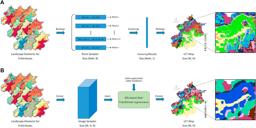
Figure 1. Illustration on the clustering process of the proposed method versus the traditional method. (A) Traditional LCA Clustering Pipeline. (B) The proposed LCA Clustering Pipeline.

To tackle this challenge, this paper introduces SwinClustering, a novel paradigm for LCA based on the advanced Swin Transformer architecture, which leverages its powerful capabilities in visual recognition and feature extraction. By employing a visual segmentation method, SwinClustering achieves multi-scale clustering, effectively capturing the diverse characteristics of landscapes across various attributes. Crucially, SwinClustering utilizes nine key attributes of landscape character maps—Altitude, Aspect, Geology, Landcover, Landform, Relief, Slope, Soil, and Vegetation—to comprehensively analyze landscape characteristics. In order to reflect the geographic location correlation between different landscape samples, SwinClustering incorporates the physical altitude, latitude and longitude information from GIS into the learning process of the model as well. Through the GIS-aware Swin Transformer backbone network, semantic features are extracted, capturing the inherent relationships and spatial patterns within and among different landscape elements. Additionally, the Feature Pyramid Decoder is leveraged for segmentation clustering, enabling a coarse-grained and fine-grained analysis of LCTs. To validate the effectiveness of SwinClustering, this paper selects three distinct scales for training and validation: the national scale of China, representing a comprehensive and diverse macro-level perspective across a vast territory; the municipal scale of Beijing Municipality, representing a larger urban landscape, and the district scale of Wuyishan National Park in Fujian Province, representing a more natural and ecologically diverse landscape. The promising results obtained from these experiments highlight the versatility and adaptability of the proposed LCA method across diverse geographic scales.

Importantly, the SwinClustering paradigm represents a unified clustering framework that deeply learns the intrinsic connections between different landscape attributes and the spatial relationships between various geographic locations. It can adopt any semi-supervised label generation module as the guidance to achieve high quality clustering. Furthermore, its strong generalization capabilities enable seamless application to LCA tasks at arbitrary scales, marking a significant advancement in the field of LCA. By leveraging the power of deep learning and visual segmentation, This unified approach paves a new way forward for a more comprehensive and accurate assessment of landscape characters.

2 Materials and methods

2.1 Study areas

This study aims to explore the variations of landscape characters at three different scales, i.e., national scale, municipal scale and district scale. At the national scale, China is selected to provide a comprehensive perspective across diverse landscapes; at the municipal scale, Beijing Municipality serves as the research area, representing a complex urban environment; and at the district scale, Wuyishan National Park in Fujian Province becomes the focal area of the investigation, highlighting a natural and ecologically rich setting. The study areas are shown in Figure 2.

Figure 2

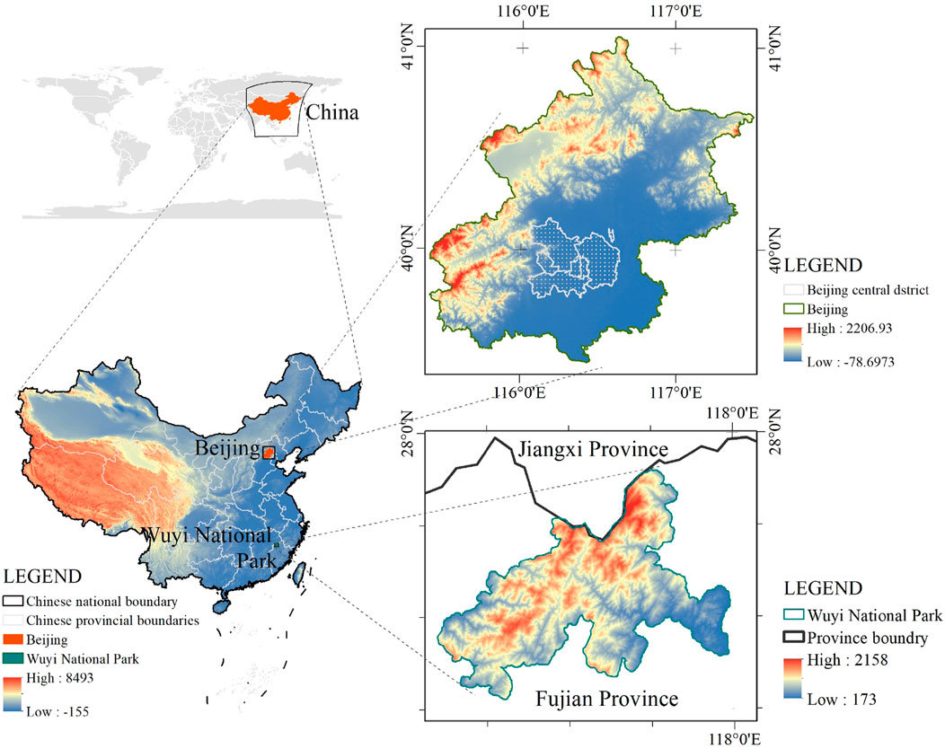
Figure 2. The study areas at different scales.

At the national scale, the study area encompasses the entire landmass of China, with a total area of approximately 9.6 million ${\text{km}}^2$. This vast expanse integrates a complex array of climatic environments, as well as diverse natural, geographical, and human resources, offering a rich landscape for analysis. China’s topography is distinguished by a general east-high, west-low gradient, forming a three-tiered elevation system that gradually steps down from the western plateau to the eastern plains. Approximately 69.2% of China’s land area consists of mountains, plateaus, and hills, while basins and plains account for the remaining 30.8%. The country’s mountainous terrain is predominantly oriented along east-west and northeast-southwest axes, shaping the landscape and influencing regional climatic patterns. This varied topography, along with the geographical and cultural diversity, makes China an ideal region for studying landscape character and its underlying drivers.

Situated in the northern reaches of China’s North Plain, Beijing Municipality spans a geographical range from $115°{25}^{\prime }$E to $117°{30}^{\prime }$E and $39°{26}^{\prime }$N to $41°{03}^{\prime }$N, encompassing approximately 16,410.54 ${\text{km}}^2$. Its terrain exhibits a distinct gradient, with the northwest exhibiting higher elevations and the southeast gently sloping towards the Bohai Sea. On its western, northern, and eastern borders, Beijing is flanked by the Taihang and Yanshan Mountains, where famous landmarks like the Badaling and Mutianyu sections of the Great Wall stand a midst lush vegetation and wildlife. Conversely, the southeastern region comprises a vast, gently sloping plain, studded with farmland, offering a stark contrast to the mountainous terrain.

On the other hand, Wuyishan National Park is situated in Nanping City, Fujian Province, China, with geographical coordinates ranging from $117°{24}^{\prime }$E to $117°{59}^{\prime }$E and $27°{31}^{\prime }$N to $27°{55}^{\prime }$N, covering an area of approximately 1,001.29 ${\text{km}}^2$. Located in the northern section of the Wuyishan Mountain Range, the park encompasses multiple nature reserves, scenic areas, and other vital ecological regions. The natural landscape of Wuyishan National Park is magnificent and diverse, boasting various vegetation types such as evergreen broad-leaved forests and mixed coniferous and broad-leaved forests, as well as abundant fauna and flora resources.

2.2 The SwinClustering framework

The overall framework of the proposed method is depicted in Figure 3, which mainly consists of four parts: data concatenation, GIS-aware Swin Transformer backbone, feature pyramid decoder, and a fusion decision-making module. Initially, we first concatenate the landscape character elements of nine attributes together through a concat operation. The concatenated features and GIS information are then fed into the GIS-aware Swin Transformer backbone, yielding multi-level feature representations. These multi-level features undergo further processing via the feature pyramid decoder, emerging as data vectors with uniform scale and channel count. Ultimately, a decision-making fuse layer outputs clustering results derived from segmentation. In the forthcoming sections, we delve into the specifics of SwinClustering’s core modules.

Figure 3

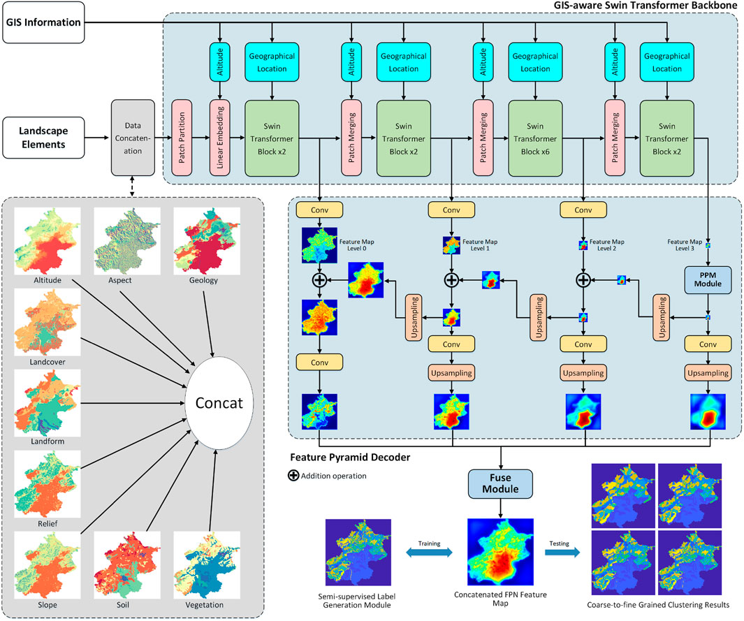
Figure 3. The overall framework of SwinClustering.

2.2.1 Data preparation

We utilize nine types of landscape attributes as input data for the network, which are Altitude, Aspect, Geology, Landcover, Landform, Relief, Slope, Soil, and Vegetation. The elements in each attribute represent a landscape representation of the area, and the visual pseudo-colour display of these landscape elements is shown in the left bottom of Figure 3. The data details and data sources of these landscape attributes in this paper are shown in Table 1. Altitude data originate from NASA EARTHDATA, whereas slope, aspect, and relief data are derived from altitude calculations. Geology bedrock data are sourced from the Geoscientific Data & Discovery Publishing System (Ye et al., 2017). Soil (Gao and Li, 2000) and landform (Zhou and Cheng, 2019) datasets are retrieved from the National Earth System Science Data Center. Vegetation data are collected from the National Cryosphere Desert Data Center (Editorial Committee of Chinese Vegetation MapC. A. o. S., 2023), and landcover data are acquired from Earth System Science Data (Yang and Xin, 2023). Notably, all data pertaining to Beijing and Wuyishan National Park share the same sources.

Table 1

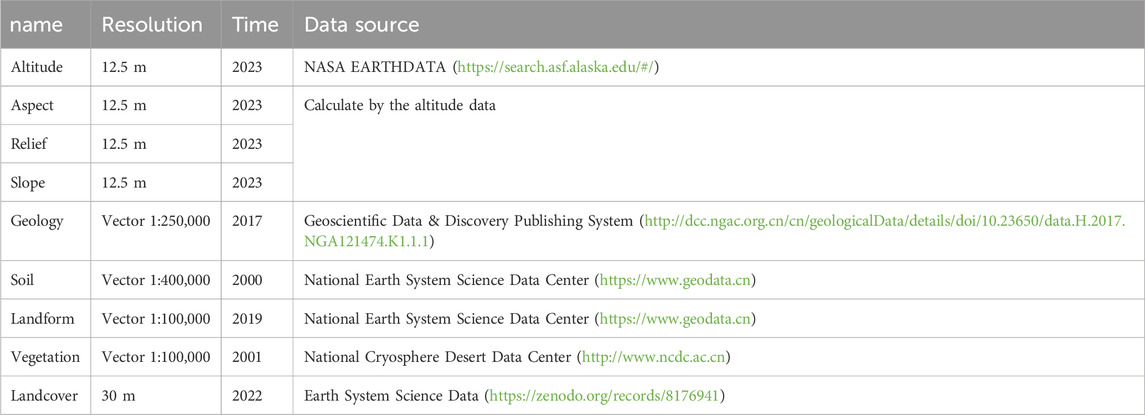
Table 1. Data details and data sources.

In the pre-processing stage, we first scale these nine landscape attribute feature maps to the same size, i.e., the China region is scaled to a resolution of $5186\times 5255$, the Beijing region is scaled to a resolution of $3552\times 3660$, and the Wuyishan region is scaled to a resolution of $2381\times 1400.$ Because the landscape attribute data from different sources have deviations in their corresponding boundaries, we then perform boundary alignment, where we set the region where all nine attributes have valid landscape elements as the boundary selection condition for the input data boundary alignment. Finally, we combine the nine attribute channel together and normalize the landscape data to ensure that each attribute feature acts uniformly in the clustering decision process. The pseudo-coloured feature maps of the nine attributes after preprocessing are shown in the left bottom of Figure 3.

2.2.2 GIS-aware Swin Transformer backbone

Currently, the most popular semantic learning models in vision are divided into those based on CNN (Li et al., 2021) and those based on Transformers (Vaswani et al., 2017). CNN networks have significant advantages in extracting local semantic features at the block level, while Transformer networks are specialized in capturing global semantic information. While Swin Transformer (Liu et al., 2021b) combines the advantages of both. The main innovation of the Swin Transformer lies in its adoption of a technique called “Shifted Windows,” which fully utilizes global and local information through non-overlapping local windows and overlapping cross windows, thereby enhancing the model’s expressive power and adaptability. Given the outstanding performance of the Swin Transformer in the vision field, this paper proposes to adopt the Swin Transformer architecture as the semantic feature extractor.

2.2.2.1 Self-attention

The standard Transformer architecture is primarily based on the attention mechanism, which leverages an attention function to map queries and a set of key-value pairs to an output. Inputs to this mechanism include queries $(Q)$, keys $(K)$, and values $(V)$, with the keys and values being processed together for efficient computation. The similarity between queries and keys is determined through a process known as Self-Attention (SA), which is computed using Equation 1.

$SA\left(Q,K,V\right)=Softmax\left(\frac{Q{K}^{\mathsf{T}}}{\sqrt{d_k}}+B\right)V,(1)$

where $d_k$ is the key dimension, and $B$ represents the relative position bias.

The self-attention mechanism can be extended to a multiple-head version, enabling the model to jointly learn various semantic information from different representation subspaces at different positions. This Multiple-head Self-Attention (MSA) mechanism can be implemented through concatenation and linear projection, which is computed using Equation 2.

$MSA\left(Q,K,V\right)=Concat\left(J_1,\dots ,J_h\right)P^O,(2)$

where $J_i=SA(Q{P}_i^Q,K{P}_i^K,V{P}_i^V)$, and $P_i^Q\in R^{d_m\times d_k}$, $P_i^K\in R^{d_m\times d_k}$, $P_i^V\in R^{d_m\times d_v}$, $P^O\in R^{h{d}_v\times d_m}$ are projection parameter matrices.

2.2.2.2 GIS information Integration

During the LCA process, we consider the impact of two GIS factors on landscape clustering: i) Altitude significantly affects the landscape elements. The model should assign different weights based on altitude, and thus the Swin Transformer backbone should have altitude awareness. ii) The geographical longitude and latitude of feature samples also heavily influence landscape characters. Unlike traditional classification tasks, each sample in LCA is not independent but has geospatial correlation. Thus, the Swin Transformer backbone should also have geographical location awareness.

To achieve altitude awareness, we input the altitude as a priori weight map into the model. Assuming the altitude priori weight map is denoted as $\omega \in R^{N,H,W}$, where $N$ is the batch size, $H$ and $W$ are the image size. We first reshape the weight map $\omega$ into one-channel vector ${\omega }^{\prime }\in R^{N,H\times W,1}$ to meet the requirements of one-dimensional Transformer computation. Then, we downsample ${\omega }^{\prime }$ to a size of $(N,H_i\times W_i,1)$ via Swin transformer feature extractor, here $H_i$ and $W_i$, $i\in \{\mathrm{1,2,3,4}\}$ denote the Transformer feature size for each layer. Finally we dot-multiply the weights with the transformer input feature $K$ and $V$ of each layer respectively to obtain altitude-encoded features. The altitude-aware information integration process is shown in Figure 4.

Figure 4

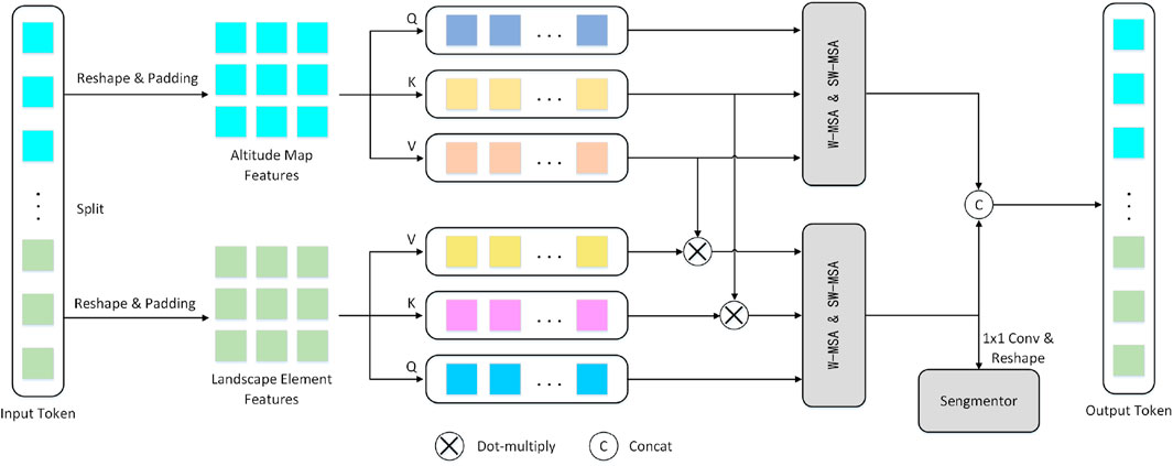
Figure 4. Altitude-aware information integration process.

To achieve geographical location awareness, we incorporate the world coordinates of each sample into the network input. When calculating similarity, the Swin Transformer adopts a relative position encoding bias to reflect the positional relationships between different patches. Each sample is independent and shares the same relative position encoding weights. However, in the LCA clustering process, there are also geographical positional relationships between samples in addition to the relative positional bias between patches. Therefore, we incorporate absolute geographical position bias into the network’s learning process. To this end, we divide $B$ in Equation 1 into two parts: $B_r$ and $B_a$, representing the relative position encoding between patches and the absolute position encoding of samples, respectively. Finally, the two tensors $B_r$ and $B_a$ are built on all pairs of tokens. The final attention is thus as shown in Equation 3.

$SA\left(Q,K_{\omega },V_{\omega }\right)=Softmax\left(\frac{Q{K}_{\omega }^{\mathsf{T}}}{\sqrt{d_k}}+B_r+B_a\right)V_{\omega },(3)$

where $K_{\omega }$ and $V_{\omega }$ denote the keys and values after latitude coding, respectively.

2.2.3 Feature pyramid network based segmentation clustering

2.2.3.1 Feature pyramid network

Utilizing the backbone network of GIS-aware Swin Transformer, we can establish a four-layer feature pyramid, with the feature dimensions being $\{\mathrm{96,192,384,768}\}$, respectively. To overcome the issue raised by Zhou et al. (2014) that the empirical perception of global semantic features is insufficient in deep network features, we employ a Pyramid Pooling Module (PPM) as a bottleneck module to bridge the decoder module of the multi-layer pyramid (Xiao et al., 2018). The PPM module, which is borrowed from PSPNet (Zhao et al., 2017), takes the features of the last layer of GIS-aware Swin Transformer $(768\times H/32\times W/32)$ as input to capture global prior representational information. Additionally, a $3\times 3$ convolution layer is employed within the PPM module, which unifies the output feature vector dimension to 512, serving as the fundamental feature for the feature upsampled pyramid.

2.2.3.2 FPN based decoder for segmentation

To achieve the fusion of multi-channel features, we first apply a $1\times 1$ convolution to the GIS-aware Swin Transformer features of each stage (excluding the bottom bottleneck stage), converting their feature channel dimension to 512. Subsequently, starting from the output of the PPM module, we perform a linear interpolation upsampling operation to expand the feature size and additively merge them with the features of the previous stage. Then, a $3\times 3$ convolution is applied to the merged feature vectors of each stage, followed by another linear interpolation operation to ensure that all features are resized to match the size of the top-level features. Finally, segmentation and clustering are achieved for each location through concatenation operations and a fully connected layer. The detailed segmentation process is shown in Figure 5.

Figure 5

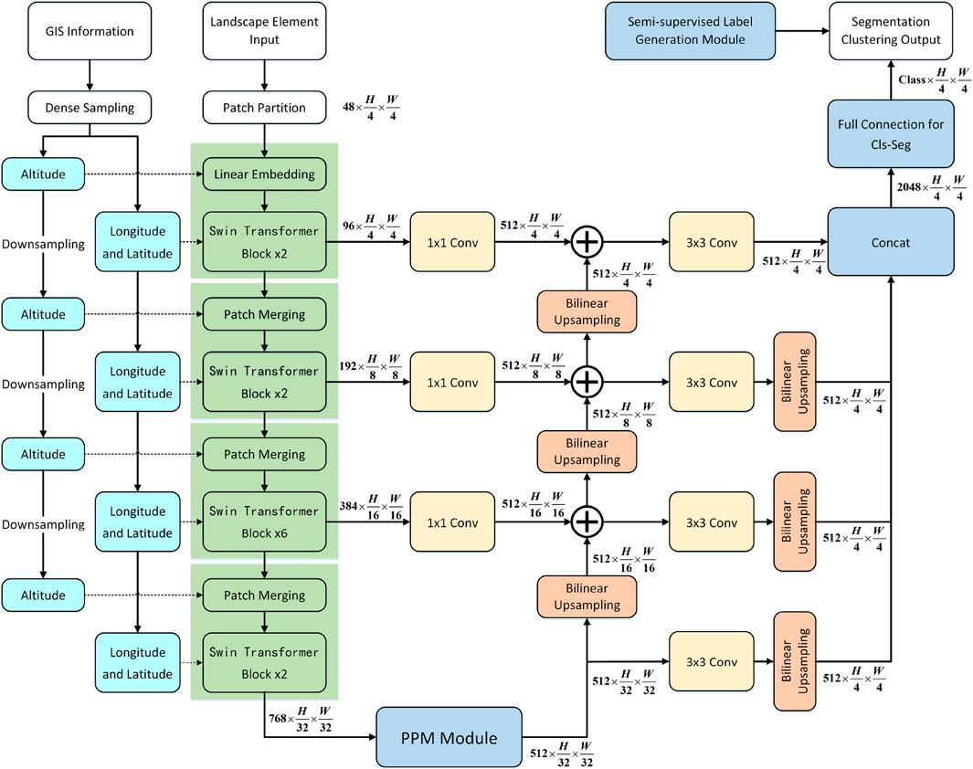
Figure 5. Illustration of the FPN based segmentation clustering process.

2.2.4 Semi-supervised label generation

In our landscape character clustering task, we do not possess manually annotated uniform labels. Instead, we employ a semi-supervised label generation module to generate pseudo-label data, which serves as guidance for the network training. Our semi-supervised label generation method adopts PCA downscaling and K-means clustering as the key techniques, and thus we name it PCA-K-means.

The K-means-based method has two major limitations: i) it needs to calculate the distance matrix between every two samples, so it cannot handle large-scale sample clustering tasks (e.g., the size of the distance matrix for the original resolution of the Beijing region is: (3552 × 3660, 3552 × 3660), which is so huge that it can hardly be calculated); ii) Each sample point is independent of each other and there is a lot of noise in the clustering results.

Since K-means based methods cannot handle large-scale sample clustering, we first reduce the size of the image to 1/6 of its original size for label generation. Then our PCA-K-means implements PCA analysis to compress the number of feature channels from nine dimensions to five dimensions, and performs K-means clustering on the compressed image data. Finally, these clustering labels are scaled up to the original image size using nearest neighbour interpolation. PCA-K-means can generate clustering results with less noise by PCA dimensionality reduction. Consequently, by altering the number of categories in the pseudo-label data, we can control the final output category number of the model, and the demonstrating experiments will be presented in Section 3.4. In addition, we can also use other clustering methods such as GMM (Stauffer and Grimson, 1999), OMSC (Chen et al., 2022) to guide the generation of pseudo labels and we will verify this in Section 3.5.

2.2.5 Coarse-grained and fine-grained training strategy

In order to meet the needs of landscape management, it is necessary to divide the landscape attributes to varying degrees of coarseness and fineness. The clustering results of LCA analysis with multiple attributes are often complex and discontinuous. This makes the subsequent landscape zoning difficult and cumbersome. To solve this problem, this paper proposes a coarse-grained and fine-grained training strategy, which can achieve the control of clustering fineness without relying on any human involvement or the burden of additional computation.

Transformer has the ability of global perception, and if given a training sample with diverse landscape character types, it will take full account of the global diversity and thus output the complex labels. On the contrary, if the training sample character types are simple, the trained model will also try to give less complex outputs even when faced with the complex testing samples of diverse character types. Thus we can regulate the degree of coarseness and fineness of the clustering output based on this property of Transformer. Suppose the size of the landscape feature map we need to cluster is $(N,9,H,W)$, where $N$ denotes the number of samples, $(H,W)$ denotes the image resolution, and 9 denotes the attribute channel. The original feature map is often very large and have complex landscape character types, it can be divided into smaller patches where there will be fewer landscape character types in each patch, and thus the complexity will be reduced. In order to make the clustering/segmentation more coarse, we divide the image resolution by $(n,n)$, so we can get the new training landscape feature map of size $(N\times n\times n,9,H/n,W/n)$, where $N\times n\times n$ denotes the number of samples, $(H/n,W/n)$ denotes the image resolution. By controlling the value of $n$, we can control the coarseness and fineness of the output.

2.2.6 Loss function

In this paper, we adopt the most typical Cross Entropy Loss as the loss function of the network, and its calculation formula is showing in Equation 4.

$\mathcal{L}=\frac{1}{N}{\displaystyle \sum _i}{\mathcal{L}}_i=-\frac{1}{N}{\displaystyle \sum _i}{\displaystyle \sum _{c=1}^M}{y}_{ic}\log \left(p_{ic}\right)(4)$

where $M$ represents the number of categories. $y_{ic}$ is a binary function for labels, which takes the value of 1 if the true category of sample $i$ is equal to $c$, and 0 otherwise. $p_{ic}$ denotes the predicted probability that the observed sample $i$ belongs to category $c$.

For each sample, the model first converts the raw output into a probability distribution through the FPN decoder. Then, it calculates the negative logarithm of the probability corresponding to the true label and accumulates the losses across all categories. As a result, when the model’s predicted probability is higher, the loss is smaller; conversely, if the predicted probability is lower, the loss is larger.

3 Results and discussions

3.1 Experimental settings

The experiments are conducted on an Ubuntu 22.04.4 LTS server equipped with an Intel(R) Xeon(R) CPU E5-2687W v3 @ 3.10 GHz and an NVIDIA TITAN RTX 24G GPU. The main programming language used for the experiment is Python 3.8.1, with CUDA version 11.1 and torch version 1.8.1. Data analyses are done in Matlab 2022a. The sliding window size of the Swin transformer backbone network is set to 7.0, and the number of Swin transformer blocks in the four stages are 2, 2, 6 and 2, respectively. The AdamW (Loshchilov and Hutter, 2017) optimizer is used for training, with a total of 15,000 iterations. The learning rate, weight decay, and beta values (${\beta }_1$ and ${\beta }_2$) are set to 0.00006, 0.01, and (0.9, 0.999), respectively.

3.2 Training overview

To accelerate the convergence speed of training, we initialize the backbone weights using pre-trained weights from ImageNet-1K (Liu et al., 2021b). The multi-attribute landscape data from the Beijing region are employed for training with a total of 3500 iterations, and validation evaluations are conducted every 500 iterations. Due to the absence of manually annotated data, we also set the K-means guided pseudo-label data as the reference groundtruth and apply the following three metrics for validation:

3.2.1 Mean intersection over union

mIoU refers to the average value of IOU for all categories. For landscape element segmentation, we compare the predicted label of each pixel with the true label and then calculate the IOU between them. Thereby, mIoU evaluates the segmentation accuracy of the model across different categories.

3.2.2 Average accuracy

aAcc refers to the average pixel classification accuracy of the model. aAcc can be used to evaluate the overall accuracy in pixel classification, but it cannot reflect the performance differences between different categories.

3.2.3 Mean accuracy

mAcc calculates the accuracy of each individual category first and subsequently takes the average of them. mAcc assesses the performance differences between different categories and it can reflect the overall performance of the model across multiple categories.

The training loss and the values of these three validation metrics are shown in the Figure 6. It can be observed that the model converges well at approximately 3,000 iterations. The visualization of segmentation clustering during training process is also shown in Figure 6. The number of iterations for the visual clustering results are (500, 1000, 1500, 2000, 2500, 3000), and it can be seen that as the number of iterations increases the clustering results become more refined.

Figure 6

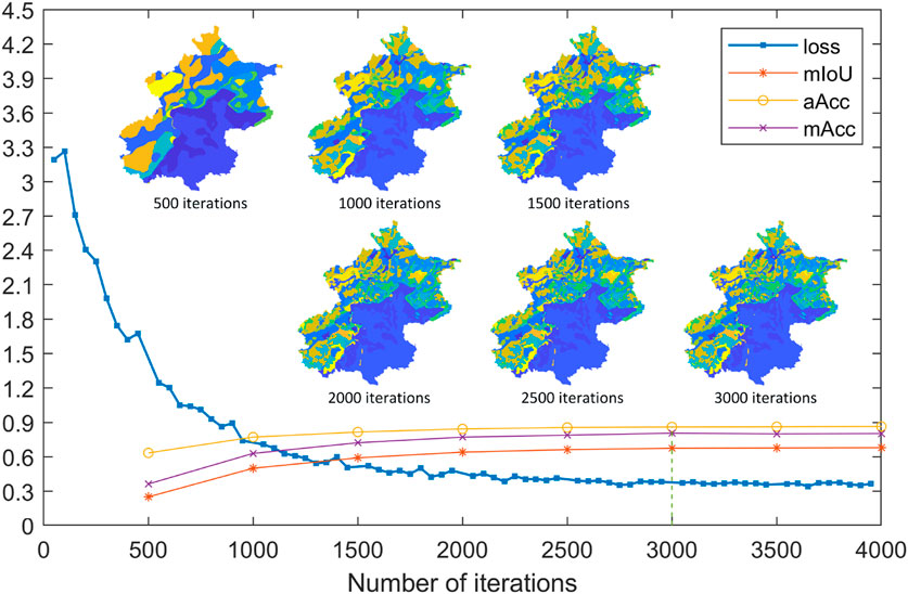
Figure 6. Visualization of loss, mIoU, aAcc, mAcc and segmentation clustering results during the training process.

3.3 Coarse-grained and fine-grained comparisons

In clustering analysis, granularity of data pertains to the level of aggregation and intricacy among data elements. Coarse-grained clustering involves grouping landscape elements into larger, more comprehensive clusters, exhibiting distinct differences between clusters. Conversely, fine-grained clustering segregates landscape elements into smaller, more specific clusters, where samples within each cluster exhibit greater similarity and subtler differences between clusters.

Most clustering techniques lack the ability to effectively regulate the degree of coarseness and fineness in clustering outcomes. However, the proposed method introduces a specialized training strategy that allows for precise control over the coarseness and fineness of the outputs. Precisely, we manipulate the fineness of clustering by partitioning the input samples. In this experiments, we partition the input samples into patches of varying sizes, i.e., $1\times 1$, $2\times 2$, $3\times 3$, $4\times 4$, $5\times 5$, and $6\times 6$, to obtain corresponding clustering maps. The visualized clustering results at 3000 iterations are as illustrated in Figure 7. It becomes evident that as the number of partitions increases, more landscape character elements are present in each individual sample, leading to coarser clustering results.

Figure 7

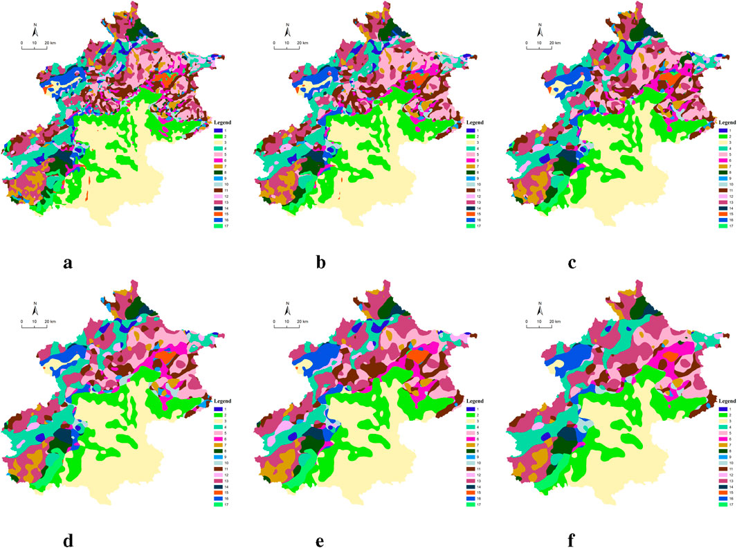
Figure 7. (A) Category 7. (B) Category 10. (C) Category 12. (D) Category 15. (E) Category 17. (F) Category 20. Fine-grained and coarse-grained comparisons at 3000 iterations.

3.4 Analysis with different number of clusters

In this section, we present the effect of the model on the processing of different number of clusters. The Beijing regional landscape character data are selected as the samples for training and testing. The coarseness-fineness controlling factor is set to $1\times 1$, and the testing models are training with 3000 iterations, and the number of clusters is set to (7, 10, 12, 15, 17, 20).

The visualisation of the clustering results with PCA-K-means guidance for different number of clusters is shown in Figure 8. From the figure, we see that these boundaries become smooth and there is less noise in the clustering results via training with SwinClustering. In addition, we can conclude that the more the number of clusters the more complex the landscape elements. Furthermore, we find that the main landscape character regions will not change with the number of clusters, for example, the shallow mountainous areas in the left top and the urban areas in the right bottom are not significantly changed. The variations of the training loss with different number of clusters are shown in Figure 9. We reach a conclusion from these loss curves: as the number of clusters increases, the more complex the landscape elements are, but the training convergence of SwinClustering does not slow down accordingly. Consequently, although increasing the number of clusters can severely increase the computational burden in the conventional clustering algorithms, our SwinClustering method is not affected by the increase in the number of clusters at all, and the speed of training convergence is not correlated with the number of clusters.

Figure 8

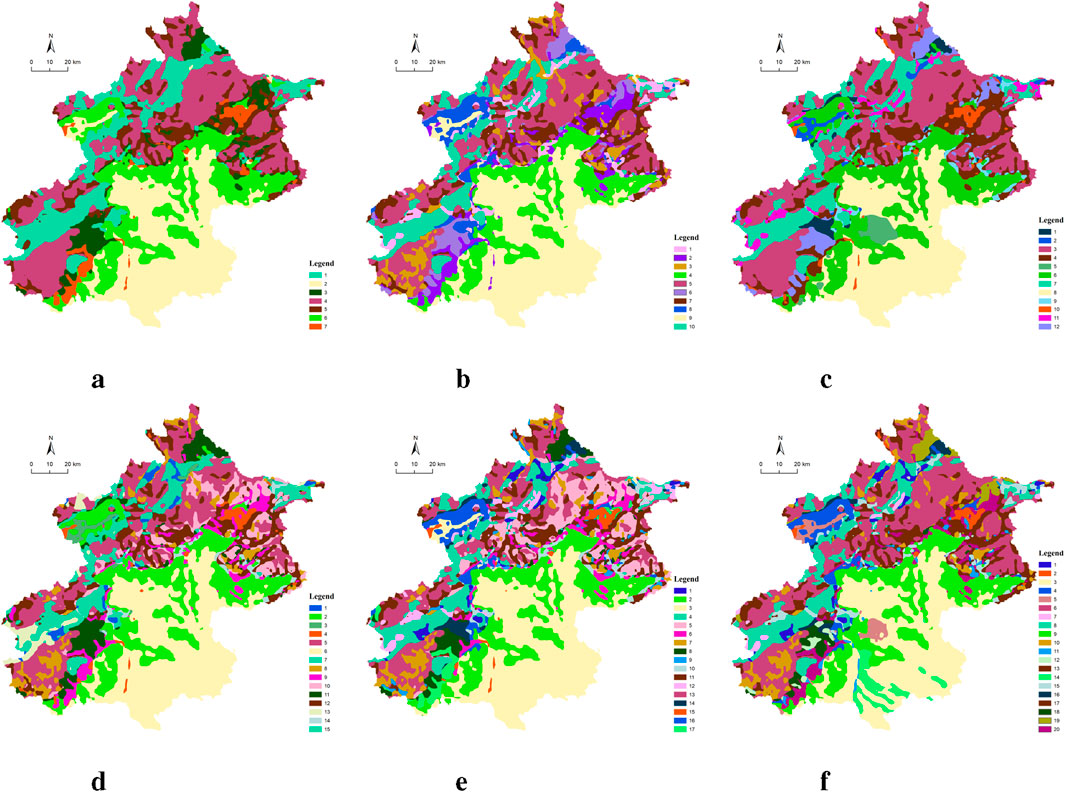
Figure 8. (A) Category 7. (B) Category 10. (C) Category 12. (D) Category 15. (E) Category 17. (F) Category 20. SwinClustering output for different number of clusters: the number of clusters are (7, 10, 12, 15, 17, 20).

Figure 9

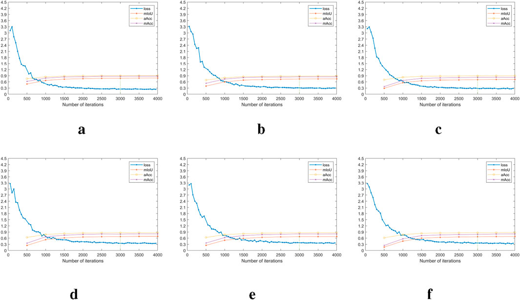
Figure 9. (A) Category 7. (B) Category 10. (C) Category 12. (D) Category 15. (E) Category 17. (F) Category 20. Curves of loss, mIoU, aAcc and mAcc with for different number of clusters: the number of clusters are (7, 10, 12, 15, 17, 20).

3.5 Analysis of clustering effects guided by different labels

In this part, we present the effect of different guided labels on the clustering results of SwinClustering. SwinClustering is a flexible segmentation clustering framework that allows the clustering generation to be guided by arbitrary other labels. This experiment removes the SwinClustering pseudo-labelled generation model directly, and then loads the clustering results of the four algorithms to guide the training of the model, which are GMM (Stauffer and Grimson, 1999), OMSC (Chen et al., 2022), OPMC (Liu et al., 2021a), and EEO (Wang et al., 2023). The number of clusters is set to 17, fine-grained and coarse-grained control parameter is set to $1\times 1$, and all parameters of the training are kept unchanged. Note that none of the labels generated in this section have been processed by PCA.

Figure 10 shows the clustering effect of SwinClustering guided by different labels. The top row of Figures 10A–D represent the clustering results generated by different clustering methods; the middle row of Figures 10E–H represent the clustering outputs of the SwinClustering at 3000 iterations; and the bottom row of Figures 10I–L represent the changes in the loss function curves during the training process. From these figures we can conclude that i) the clustering results can be de-noised well by SwinClustering, ii) SwinClustering can remove the discontinuity or jaggedness of cluster-cluster boundaries well, and iii) using other types of guiding labels does not affect the convergence speed of SwinClustering.

Figure 10

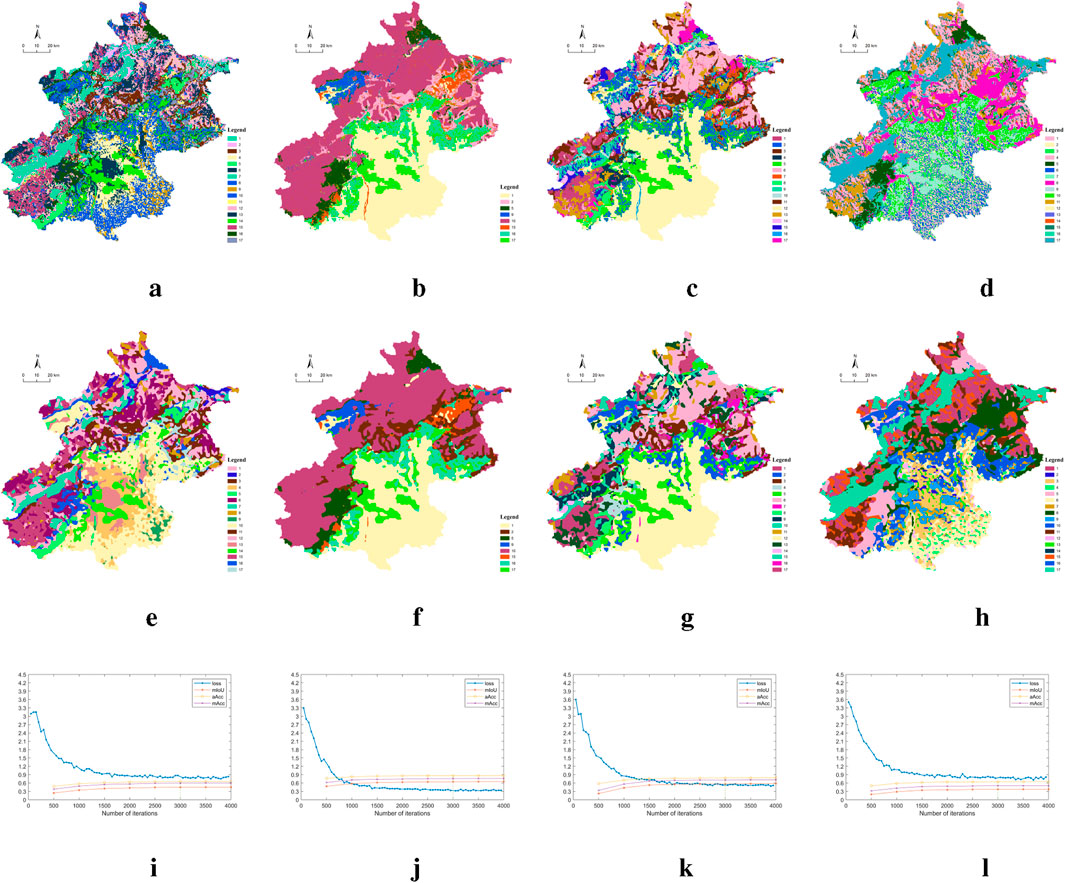
Figure 10. (A) GMM Guidance Labels. (B) OMSC Guidance Labels. (C) OPMC Guidance Labels. (D) EEO Guidance Labels. (E) GMM Guided SwinClustering. (F) OMSC Guided SwinClustering. (G) OPMC Guided SwinClustering. (H) EEO Guided SwinClustering. (I) GMM Guided Loss Variations. (J) OMSC Guided Loss Variations. (K) OPMC Guided Loss Variations. (L) EEO Guided Loss Variations. Comparison of clustering performance of SwinClustering method with different label guidance.

3.6 Quantitative evaluation

The clustering performance is often quantitatively evaluated by using the following eight evaluation metrics: ACC, NMI, Purity, Precision, Recall, F-score, ARI, and Entropy. In this experiment, we adopt the semi-supervised PCA-K-means label generation model output as the reference ground truth, and the number of clusters for all algorithms is set to 17. Since pseudo-label data generated by PCA-K-means is not the true labels, and there is no fixed uniform criterion for LCA, so the quantitative assessment methods do not distinguish better or worse. The evaluation results only measure the similarity between the clustering results and the reference pseudo-label data, which do not serve as an evaluation criterion for good or bad clustering LCA. Figure 11 demonstrates a comparative analysis of clustering results across the mentioned seven metrics. Additionally, we introduce an area metric $S$ to evaluate the overall performance of clustering algorithms. This area metric $S$ represents the total area enclosed by the spider chart, where a larger value indicates the clustering results are more similar to the reference labels. In comparison with seven representative algorithms, namely, GMM (Stauffer and Grimson, 1999), K-means (Arthur and Vassilvitskii, 2007), SOFM Kohonen (1990), OMSC (Chen et al., 2022), OPMC (Liu et al., 2021a), SFMC (Li et al., 2022), SLIC (Achanta et al., 2012) and EEO (Wang et al., 2023), the proposed SwinClustering achieves the highest scores in all metrics, i.e., ACC (0.863), NMI (0.753), Purity (0.863), F-score (0.835), Precision (0.832), Recall (0.839), and ARI (0.672). SwinClustering also secures the first place in the overall area metric with a score of $S=1.873$. Although SLIC is also a clustering method based on geographic information, it achieves the lowest score of $S=0.126$ in this quantitative evaluation. These results show that SwinClustering achieves a high fit by training with reference labels, demonstrating the capability of SwinClustering for clustering landscape elements and validating the potential of applying visual segmentation to LCA.

Figure 11

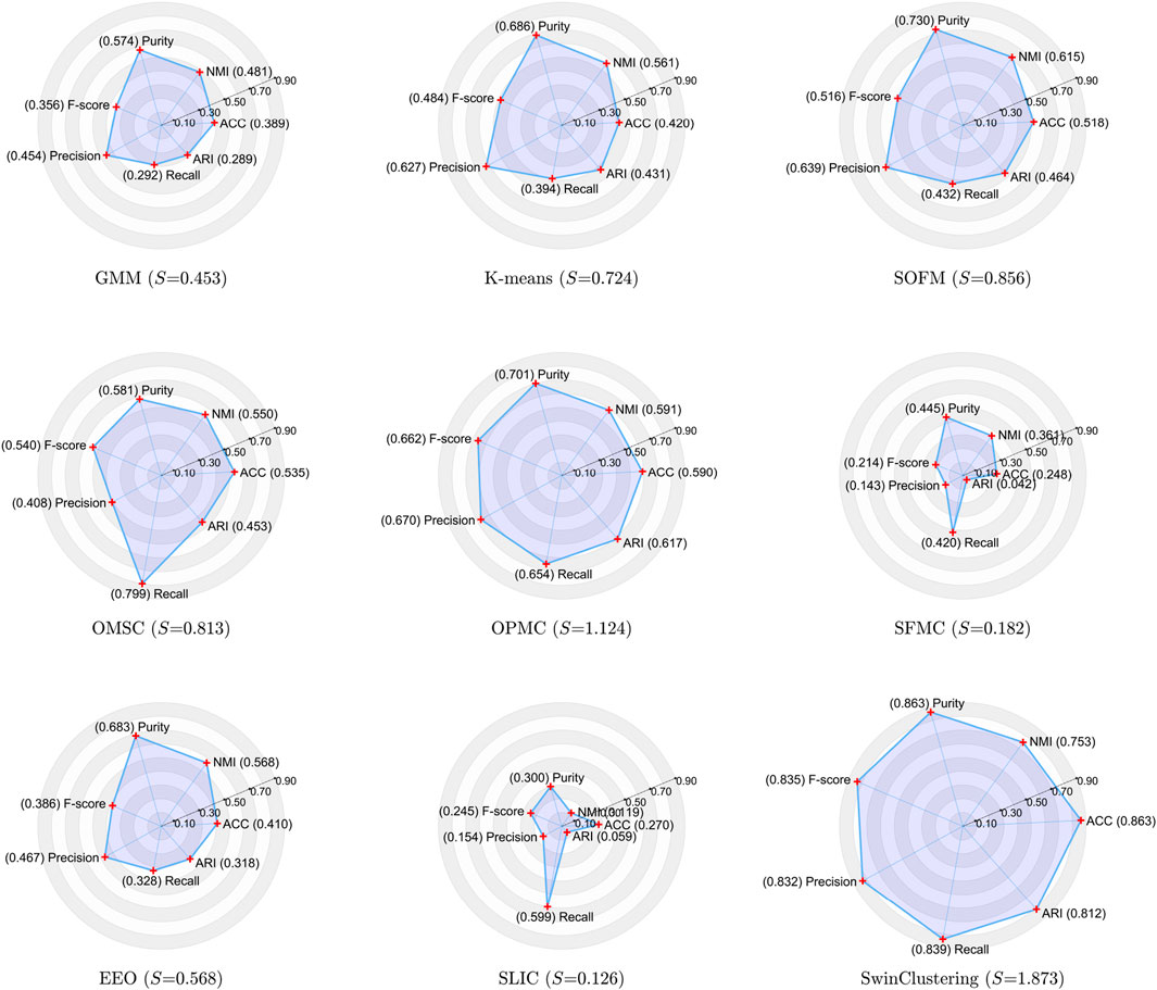
Figure 11. Comparison of the clustering performance of multiple algorithms across seven metrics: ACC, NMI, Purity, F-score, Precision, Recall and ARI.

3.7 Multi-scale qualitative analysis

We conduct experiments on qualitative LCA clustering analysis at three different scales: the national scale of China, the municipal scale of Beijing Municipality, and the district scale of Wuyishan National Park. The national scale encompasses the entirety of China, showcasing the rich and diverse landscape characteristics across various geographic regions. To better reflect this diversity, the number of clusters for the national scale is set to 80. The Beijing region, covering an area of 16,410.54 square kilometers, includes multiple landscape elements such as mountains, lakes, and urban architecture, representing a complex urban environment. The Wuyishan region, with a size of 1,001.29 square kilometers, primarily features vegetation, mountains, and water bodies, highlighting a natural and ecologically rich setting. For both the municipal and district scales, the number of clusters is set to 17. In our landscape character clustering assessment experiments, we adopt a visual qualitative comparison method to perform cluster analysis on a series of complex and variable landscape characters. For methods that cannot handle large-scale samples, we apply a reduction-computing-enlargement processing strategy.

The visual assessment results for the national scale (China) are presented in Figure 12. At this scale, the clustering results reflect the rich diversity of landscape features across the vast geographic territory of China, including urban areas, farmland, forests, mountains, deserts, and water bodies. Visual comparisons with GMM (Stauffer and Grimson, 1999), K-means (Arthur and Vassilvitskii, 2007), SOFM (Kohonen, 1990), OMSC (Chen et al., 2022), OPMC (Liu et al., 2021a), SFMC (Li et al., 2022), EEO (Wang et al., 2023), SLIC (Achanta et al., 2012), and SwinClustering are presented in Figures 12A–I. It can be observed that while most algorithms can differentiate major geographic features such as deserts in the northwest, forests in the southwest, and urban areas in the east, many suffer from excessive noise and fragmented clusters, especially GMM, K-means, and EEO. OMSC and SLIC fail to fully capture the diversity of landscape features, producing overly simplified results. In contrast, the proposed SwinClustering algorithm effectively distinguishes a wide variety of landscape types, providing smooth boundaries, well-defined clusters, and a more nuanced representation of diverse geographic regions.

Figure 12

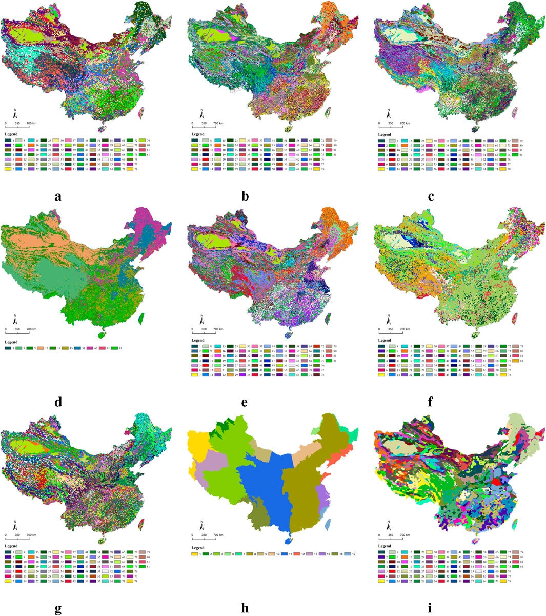
Figure 12. (A) GMM. (B) K-means. (C) SOFM. (D) OMSC. (E) OPMC. (F) SFMC. (G) EEO. (H) SLIC. (I) SwinClustering. The visual qualitative assessment results for China.

At the municipal scale, the visual assessment results for the Beijing region are presented in Figure 13. We can figure out that the southeastern part of the Beijing region primarily consists of urban architectural landscape elements, while the western and northern parts are dominated by mountainous landscape elements. Visual comparisons with GMM (Stauffer and Grimson, 1999), K-means (Arthur and Vassilvitskii, 2007), SOFM (Kohonen, 1990), OMSC (Chen et al., 2022), OPMC (Liu et al., 2021), SFMC (Li et al., 2022), EEO (Wang et al., 2023), SLIC (Achanta et al., 2012), and SwinClustering are presented in Figures 13A–I. All methods except SLIC are able to roughly segment urban and mountainous landscape elements. However, GMM, K-means and EEO tend to divide the landscape elements into finer fragments with excessive noise points. OMSC provides a rougher segmentation, resulting in the loss of many details. SOFM and OPMC distribute the landscape characters more evenly with fewer noise points, but their boundaries are not smooth, often appearing jagged. SFMC clustering results are not diverse enough and are also fraught with a lot of clutters. In contrast, our proposed method, SwinClustering, provides a more reasonable division of landscape elements with smooth boundaries and distinct blocks. It effectively represents urban architecture, vegetation, mountains, rivers, and other landscape elements, demonstrating the advanced performance of the proposed method.

Figure 13

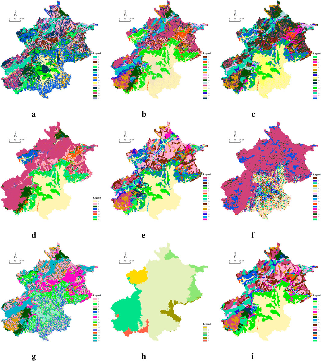
Figure 13. (A) GMM. (B) K-means. (C) SOFM. (D) OMSC. (E) OPMC. (F) SFMC. (G) EEO. (H) SLIC. (I) SwinClustering. The visual qualitative assessment results for the Beijing Municipality.

Finally, at the regional scale, the Wuyishan National Park in Fujian Province is selected for visual assessment. The landscape of the Wuyishan region is primarily characterized by its mountainous terrain, dense forests, and lush vegetation. The visual comparisons of the nine algorithms are presented in Figures 14A–I. It can be observed that GMM, OMSC, OPMC, and SwinClustering are able to clearly showcase the ridge lines in the northwest region of Wuyishan. K-means, OPMC, and SwinClustering also distinguish the different trees in the southeast region. Additionally, the proposed SwinClustering method exhibits a better overall partitioning effect, with reasonable region sizes and less noises. This fully demonstrates the application potential of visual segmentation techniques in landscape character clustering.

Figure 14

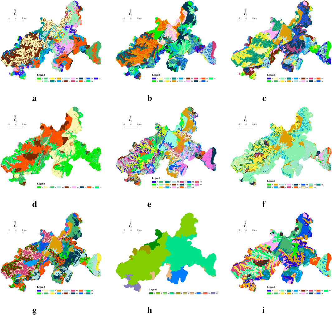
Figure 14. (A) GMM. (B) K-means. (C) SOFM. (D) OMSC. (E) OPMC. (F) SFMC. (G) EEO. (H) SLIC. (I) SwinClustering. The visual qualitative assessment results for the Wuyishan National Park.

4 Conclusion

This study highlights the importance of LCA for gaining deeper insights into multiple landscape attributes and geographic locations. The traditional LCA clustering methods have difficulty in obtaining intricate connections between different landscape attributes and in obtaining spatial relationships within the context of the scene. To achieve sustainable LCA development, we introduce SwinClustering, a novel paradigm leveraging the Swin Transformer architecture for multi-scale clustering. By validating its effectiveness across diverse scales, we successfully demonstrate the versatility and potential of SwinClustering on three distinct scales: the national scale of China, the municipal scale of Beijing, and the regional scale of Wuyishan National Park, each representing unique and diverse landscape scenarios. This study not only enhances the understanding of landscape character but also paves the way for more informed and sustainable landscape management practices via the artificial intelligence techniques.

Data availability statement

The raw data supporting the conclusions of this article will be made available by the authors, without undue reservation.

Author contributions

TH: Conceptualization, Data curation, Formal Analysis, Investigation, Methodology, Software, Validation, Visualization, Writing–original draft, Writing–review and editing. BH: Conceptualization, Formal Analysis, Funding acquisition, Methodology, Software, Supervision, Validation, Writing–original draft. SL: Funding acquisition, Investigation, Writing–review and editing. HZ: Data curation, Investigation, Writing–review and editing. XY: Data curation, Visualization, Writing–review and editing. JZ: Conceptualization, Project administration, Supervision, Writing–review and editing.

Funding

The author(s) declare that financial support was received for the research, authorship, and/or publication of this article. This work was supported by the Youth Program of National Natural Science Foundation of China (No. 62306049), the General Program of Chongqing Natural Science Foundation (No. CSTB2023NSCQ-MSX0665), the Fundamental Research Funds for the Central Universities (No. 2024CDJXY008), and the Talent Project of China University of Mining and Technology (No. 102519082).

Conflict of interest

The authors declare that the research was conducted in the absence of any commercial or financial relationships that could be construed as a potential conflict of interest.

Generative AI statement

The author(s) declare that no Generative AI was used in the creation of this manuscript.

Publisher’s note

All claims expressed in this article are solely those of the authors and do not necessarily represent those of their affiliated organizations, or those of the publisher, the editors and the reviewers. Any product that may be evaluated in this article, or claim that may be made by its manufacturer, is not guaranteed or endorsed by the publisher.

References

Achanta, R., Shaji, A., Smith, K., Lucchi, A., Fua, P., and Süsstrunk, S. (2012). Slic superpixels compared to state-of-the-art superpixel methods. IEEE Trans. Pattern Analysis Mach. Intell. 34, 2274–2282. doi:10.1109/tpami.2012.120

PubMed Abstract | CrossRef Full Text | Google Scholar

Antrop, M. (2000). Background concepts for integrated landscape analysis. Agric. Ecosyst. & Environ. 77, 17–28. doi:10.1016/s0167-8809(99)00089-4

CrossRef Full Text | Google Scholar

Antrop, M., and Van Eetvelde, V. (2017). Landscape perspectives. Holist. Nat. Landsc. 100, 1–23. doi:10.1007/978-94-024-1183-6

CrossRef Full Text | Google Scholar

Arthur, D., and Vassilvitskii, S. (2007). k-means++: the advantages of careful seeding. Soda 7, 1027–1035. doi:10.1145/1283383.1283494

CrossRef Full Text | Google Scholar

Brabyn, L. (2009). Classifying landscape character. Landsc. Res. 34, 299–321. doi:10.1080/01426390802371202

CrossRef Full Text | Google Scholar

Brown, G., and Brabyn, L. (2012a). An analysis of the relationships between multiple values and physical landscapes at a regional scale using public participation gis and landscape character classification. Landsc. urban Plan. 107, 317–331. doi:10.1016/j.landurbplan.2012.06.007

CrossRef Full Text | Google Scholar

Brown, G., and Brabyn, L. (2012b). The extrapolation of social landscape values to a national level in New Zealand using landscape character classification. Appl. Geogr. 35, 84–94. doi:10.1016/j.apgeog.2012.06.002

CrossRef Full Text | Google Scholar

Butler, A. (2016). Dynamics of integrating landscape values in landscape character assessment: the hidden dominance of the objective outsider. Landsc. Res. 41, 239–252. doi:10.1080/01426397.2015.1135315

CrossRef Full Text | Google Scholar

Chen, M.-S., Wang, C.-D., Huang, D., Lai, J.-H., and Yu, P. S. (2022). “Efficient orthogonal multi-view subspace clustering,” in Proceedings of the ACM SIGKDD conference on knowledge Discovery and data mining, 127–135.

Google Scholar

Chuman, T., and Romportl, D. (2010). Multivariate classification analysis of cultural landscapes: an example from the Czech republic. Landsc. Urban Plan. 98, 200–209. doi:10.1016/j.landurbplan.2010.08.003

CrossRef Full Text | Google Scholar

Déjeant-Pons, M. (2006). The european landscape convention. Landsc. Res. 31, 363–384. doi:10.1080/01426390601004343

CrossRef Full Text | Google Scholar

Editorial Committee of Chinese Vegetation Map, C. A. o. S. (2023). “1:1 million vegetation data set in China,” in National Cryosphere Desert Data center. doi:10.12072/ncdc.nieer.db2978.2023

CrossRef Full Text | Google Scholar

Fairclough, G., Herlin, I. S., and Swanwick, C. (2018). Routledge handbook of landscape character assessment: current approaches to characterisation and assessment

Google Scholar

Gao, Y., and Li, J. (2000). 1:400,000 soil map of China (2000). Sinomap press: National Earth System Science Data Center. Available at: https://www.geodata.cn.

Google Scholar

Gkoltsiou, A., and Paraskevopoulou, A. (2021). Landscape character assessment, perception surveys of stakeholders and swot analysis: a holistic approach to historical public park management. J. Outdoor Recreat. Tour. 35, 100418. doi:10.1016/j.jort.2021.100418

CrossRef Full Text | Google Scholar

Huang, T., Zhang, Y., Li, S., Griffiths, G., Lukac, M., Zhao, H., et al. (2023). Harnessing machine learning for landscape character management in a shallow relief region of China. Landsc. Res. 48, 1019–1040. doi:10.1080/01426397.2023.2241390

CrossRef Full Text | Google Scholar

Hughes-Allen, L., Bouchard, F., Séjourné, A., Fougeron, G., and Léger, E. (2023). Automated identification of thermokarst lakes using machine learning in the ice-rich permafrost landscape of central yakutia (eastern siberia). Remote Sens. 15, 1226. doi:10.3390/rs15051226

CrossRef Full Text | Google Scholar

Jamali, A., and Mahdianpari, M. (2022). Swin transformer and deep convolutional neural networks for coastal wetland classification using sentinel-1, sentinel-2, and lidar data. Remote Sens. 14, 359. doi:10.3390/rs14020359

CrossRef Full Text | Google Scholar

Jellema, A., Stobbelaar, D.-J., Groot, J. C., and Rossing, W. A. (2009). Landscape character assessment using region growing techniques in geographical information systems. J. Environ. Manag. 90, S161–S174. doi:10.1016/j.jenvman.2008.11.031

PubMed Abstract | CrossRef Full Text | Google Scholar

Koç, A., and Yılmaz, S. (2020). Landscape character analysis and assessment at the lower basin-scale. Appl. Geogr. 125, 102359. doi:10.1016/j.apgeog.2020.102359

CrossRef Full Text | Google Scholar

Kohonen, T. (1990). The self-organizing map. Proc. IEEE 78, 1464–1480. doi:10.1109/5.58325

CrossRef Full Text | Google Scholar

Li, G., and Zhang, B. (2017). Identification of landscape character types for trans-regional integration in the wuling mountain multi-ethnic area of southwest China. Landsc. Urban Plan. 162, 25–35. doi:10.1016/j.landurbplan.2017.01.008

CrossRef Full Text | Google Scholar

Li, X., Zhang, H., Wang, R., and Nie, F. (2022). Multiview clustering: a scalable and parameter-free bipartite graph fusion method. IEEE Trans. Pattern Analysis Mach. Intell. 44, 330–344. doi:10.1109/tpami.2020.3011148

PubMed Abstract | CrossRef Full Text | Google Scholar

Li, Z., Liu, F., Yang, W., Peng, S., and Zhou, J. (2021). A survey of convolutional neural networks: analysis, applications, and prospects. IEEE Trans. neural Netw. Learn. Syst. 33, 6999–7019. doi:10.1109/tnnls.2021.3084827

PubMed Abstract | CrossRef Full Text | Google Scholar

Liu, J., Liu, X., Yang, Y., Liu, L., Wang, S., Liang, W., et al. (2021a). “One-pass multi-view clustering for large-scale data,” in Proceedings of the IEEE international conference on computer vision, 12344–12353.

Google Scholar

Liu, Z., Lin, Y., Cao, Y., Hu, H., Wei, Y., Zhang, Z., et al. (2021b). “Swin transformer: hierarchical vision transformer using shifted windows,” in Proceedings of the IEEE international conference on computer vision, 10012–10022.

Google Scholar

Loshchilov, I., and Hutter, F. (2017). Decoupled weight decay regularization. doi:10.48550/arXiv.1711.05101

CrossRef Full Text | Google Scholar

Lu, Y., Xu, S., Liu, S., and Wu, J. (2022). An approach to urban landscape character assessment: linking urban big data and machine learning. Sustain. Cities Soc. 83, 103983. doi:10.1016/j.scs.2022.103983

CrossRef Full Text | Google Scholar

Mason, R. E., Vaughn, N. R., and Asner, G. P. (2023). Mapping buildings across heterogeneous landscapes: machine learning and deep learning applied to multi-modal remote sensing data. Remote Sens. 15, 4389. doi:10.3390/rs15184389

CrossRef Full Text | Google Scholar

Pan, Y., Wu, Y., Xu, X., Zhang, B., and Li, W. (2022). Identifying terrestrial landscape character types in China. Land 11, 1014. doi:10.3390/land11071014

CrossRef Full Text | Google Scholar

Simensen, T., Halvorsen, R., and Erikstad, L. (2018). Methods for landscape characterisation and mapping: a systematic review. Land use policy 75, 557–569. doi:10.1016/j.landusepol.2018.04.022

CrossRef Full Text | Google Scholar

Stauffer, C., and Grimson, W. E. L. (1999). Adaptive background mixture models for real-time tracking. Proc. IEEE Conf. Comput. Vis. Pattern Recognit. 2, 246–252. doi:10.1109/cvpr.1999.784637

CrossRef Full Text | Google Scholar

Swanwick, C. (2002). Landscape character assessment: Guidance for England and scotland; Prepared on Behalf of the countryside Agency and scottish natural heritage (countryside agency)

Google Scholar

Tveit, M., Ode, Å., and Fry, G. (2006). Key concepts in a framework for analysing visual landscape character. Landsc. Res. 31, 229–255. doi:10.1080/01426390600783269

CrossRef Full Text | Google Scholar

Vaswani, A., Shazeer, N., Parmar, N., Uszkoreit, J., Jones, L., Gomez, A. N., et al. (2017). Attention is all you need. Adv. Neural Inf. Process. Syst. 30. doi:10.48550/arXiv.1706.03762

CrossRef Full Text | Google Scholar

Wang, J., Tang, C., Wan, Z., Zhang, W., Sun, K., and Zomaya, A. Y. (2023). Efficient and effective one-step multiview clustering. IEEE Trans. Neural Netw. Learn. Syst. 35, 12224–12235. doi:10.1109/tnnls.2023.3253246

PubMed Abstract | CrossRef Full Text | Google Scholar

Wei, J., Yue, W., Li, M., and Gao, J. (2022). Mapping human perception of urban landscape from street-view images: a deep-learning approach. Int. J. Appl. Earth Observation Geoinformation 112, 102886. doi:10.1016/j.jag.2022.102886

CrossRef Full Text | Google Scholar

Xiao, T., Liu, Y., Zhou, B., Jiang, Y., and Sun, J. (2018). “Unified perceptual parsing for scene understanding,” in Proceedings of the European conference on computer vision, 418–434.

Google Scholar

Yang, D., Gao, C., Li, L., and Van Eetvelde, V. (2020). Multi-scaled identification of landscape character types and areas in lushan national park and its fringes, China. Landsc. Urban Plan. 201, 103844. doi:10.1016/j.landurbplan.2020.103844

CrossRef Full Text | Google Scholar

Yang, J., and Xin, H. (2023). The 30 m annual land cover dataset and its dynamics in China from 1990 to 2019. Earth Syst. Sci. Data 13, 3907–3925. doi:10.5194/essd-13-3907-2021

CrossRef Full Text | Google Scholar

Ye, T., Huang, C., and Deng, Z. (2017). Spatial database of 1:2500000 digital geologic map of people’s Republic of China [db]. Glob. Geol. Data. doi:10.23650/data.H2017.NGA121474.k.1.1

CrossRef Full Text | Google Scholar

Zhao, H., Shi, J., Qi, X., Wang, X., and Jia, J. (2017). “Pyramid scene parsing network,” in Proceedings of the IEEE conference on computer vision and pattern recognition, 2881–2890.

Google Scholar

Zhou, B., Khosla, A., Lapedriza, A., Oliva, A., and Torralba, A. (2014). Object detectors emerge in deep scene cnns. doi:10.48550/arXiv.1412.6856

CrossRef Full Text | Google Scholar

Zhou, C., and Cheng, W. (2019). 1:1,000,000 geomorphological map of western China. Natl. Tibet. Plateau Data Cent. doi:10.11888/Geogra.tpdc.270104

CrossRef Full Text | Google Scholar

Zu, X., Gao, C., and Wang, Y. (2024). Towards religious landscape: protection of Tibetan buddhist heritage in aba prefecture. Int. J. Appl. Earth Observation Geoinformation 130, 103885. doi:10.1016/j.jag.2024.103885

CrossRef Full Text | Google Scholar