Comparison of simulating visibility using XGBoost and IMPROVE method: a case study in East China

The prediction accuracy of atmospheric visibility significantly impacts daily life. However, there is a relative scarcity of research on post-processing methods for visibility obtained from the WRF-Chem atmospheric chemistry model results. In order to explore a more accurate method for visibility calculation, we conducted a study on the meteorological conditions in the East China region during a heavy pollution period from October 1 to 23 in the year of 2022. The meteorological data were processed using both the XGBoost (XGB) model and the IMPROVE to calculate visibility. The results indicate that XGB outperforms the IMPROVE in various aspects. The visibility improved from a correlation of 0.56–0.71 with the use of XGB. And in comparison with the IMPROVE equation, XGB demonstrated a statistically significant reduction in RMSE by 1.96 km. Even in regions where the IMPROVE performs poorly, XGB demonstrates superior performance. In regions where the correlation simulated by the IMPROVE equation is less than 0.2 (Anqing and Nanyang), XGB still performs well, achieving correlations of 0.69 (Anqing) and 0.68 (Nanyang). Throughout the entire study period, the average visibility results obtained by XGB deviate by only 0.07 km from the observed values. These findings underscore the importance of incorporating the XGBoost model into WRF-Chem visibility simulations, as it significantly improves the accuracy of visibility predictions.

1 Introduction

Visibility is a critical meteorological parameter with significant implications (Deng et al., 2011) in various domains, including aviation and road transportation. Visibility is essential for the safe operation of flights, in that reduced visibility can result in flight delays, cancellations, and potentially hazardous situations (Shen et al., 2023). Therefore, accurate visibility forecasting is of paramount importance to ensure the smooth functioning of flights and the safety of both pilots and passengers. Currently, research in the field of visibility focuses on predicting visibility, analyzing factors associated with it (Che et al., 2007; Gao et al., 2016), and understanding the underlying causes of reduced visibility (Chmielecki and Raftery, 2011; Guo et al., 2017; Benjamin et al., 2004; Gultepe and Milbrandt, 2010).

Currently, two primary methods are frequently used for visibility prediction. One approach utilizes statistical methods, where relevant meteorological variables are employed as predictors to construct models for visibility prediction. Previous research (Bari and Ouagabi, 2020) has shown that machine learning techniques, which incorporate multiple relevant predictors, significantly outperform models that rely solely on individual meteorological variables with high correlations. Furthermore, artificial neural networks (Colabone et al., 2015) have been utilized to address complex nonlinear relationships between variables. Various machine learning algorithms, including multi-layer perceptrons (Riedmiller, 1994) and support vector regression (Awad et al., 2015) have demonstrated commendable predictive performance for runway visibility at airports such as Valladolid (Cornejo-Bueno et al., 2017). Additionally, decision trees (Bari and Ouagabi, 2020), k-nearest neighbors (KNN) (Peterson, 2009), and neural networks (Liu et al., 2020) have been applied to predict visibility in the Chengdu region, effectively enhancing the credibility of visibility forecasts (Zhang et al., 2022). These studies underline the potential of machine learning to improve the accuracy of meteorological forecasting (Wen et al., 2023; Castillo-Botón et al., 2022; Fang et al., 2023). Previous studies (Bari and Ouagabi, 2020; Kim et al., 2022; Gao et al., 2024; Kumar et al., 2023; Xiong et al., 2022) have shown that the XGB model has unique advantages when dealing with the complex nonlinear relationship of meteorological data, and can effectively avoid overfitting. On the other hand, the XGB model is based on the gradient boosting framework, which converges faster when iteratively optimizing the loss function, and can efficiently train meteorological datasets to achieve a higher prediction level.

The other method involves numerical weather predictions, utilizing mathematical models and computer simulations based on the principles of atmospheric science and physics to forecast atmospheric and meteorological phenomena (Roman Cascon et al., 2016; Steeneveld et al., 2015). Among these numerical models, the WRF-Chem model is renowned for its exceptional performance in meteorological research (Hu et al., 2021; Sati and Mohan, 2021), primarily attributed to its consideration of aerosol-radiation interactions and aerosol-cloud interactions (Che et al., 2019; Gao et al., 2020). Researchers (Ding et al., 2016) have observed that the bi-directionally coupled WRF-Chem atmospheric chemistry model significantly enhances the simulation and prediction of air pollution concentrations, particularly in highly polluted conditions, in comparison to other numerical forecast models. Several studies (Malm and Hand, 2007; Wang et al., 2015; Deng et al., 2016) collectively validate the effectiveness of the IMPROVE empirical formula in calculating atmospheric extinction coefficients and deriving visibility information from WRF-Chem simulations. However, it is crucial to note that under hazy conditions, the IMPROVE formula may introduce biases, potentially leading to overestimation of visibility (Tao et al., 2020). In addition, the research (Peng et al., 2020) has also identified that, in high-humidity environments, the application of the IMPROVE formula leads to a significant overestimation of visibility values. These research findings indicate that the IMPROVE empirical formula falls slightly short in accounting for the light-scattering properties of fog droplets, particularly under conditions of haze and high humidity. These shortcomings significantly affect the estimation of atmospheric extinction coefficients, subsequently resulting in deviations in visibility. In conclusion, it is necessary to explore a new approach for handling meteorological elements output by the WRF-Chem model in order to enhance the accuracy of visibility predictions. This will contribute to the research on how to improve the accuracy of visibility forecasts.

The primary objective of this study is to enhance the visibility calculation method based on the WRF-Chem model, combining the flexibility of machine learning with the precision of atmospheric physics and chemical reactions in numerical simulations. Under complex conditions, this approach aims to simulate the relationships more accurately among various meteorological elements, thereby improving the accuracy of visibility predictions.

2 Model and methods

2.1 Configuration of the WRF-Chem model

The numerical simulation model employed in this study is the WRF-Chem model, which possesses the capability to provide comprehensive aerosol feedback, including aerosol-radiation interactions and aerosol-cloud interactions. Additionally, it offers a selection of various physical and chemical parameterization schemes, facilitating the tight coupling of physical and chemical processes. Thus, it is widely used in relevant research fields (Gao et al., 2017; Chen et al., 2023). For this research, meteorological initial and boundary conditions are provided by the National Center for Atmospheric Research (NCAR, https://rda.ucar.edu/). FNL data and default detailed topographic data (Download URL: https://www2.mmm.ucar.edu/wrf/users/download/get_sources_wps_geog.html) are used as input sources in the meteorological data preprocessing phase of the Weather Research and Forecasting (WRF) model. These data are processed through the “ungrib” and “geogrid” modules and then integrated into the WRF model as initial fields and boundary conditions. The specific process of data processing is shown in Figure 1.

Figure 1

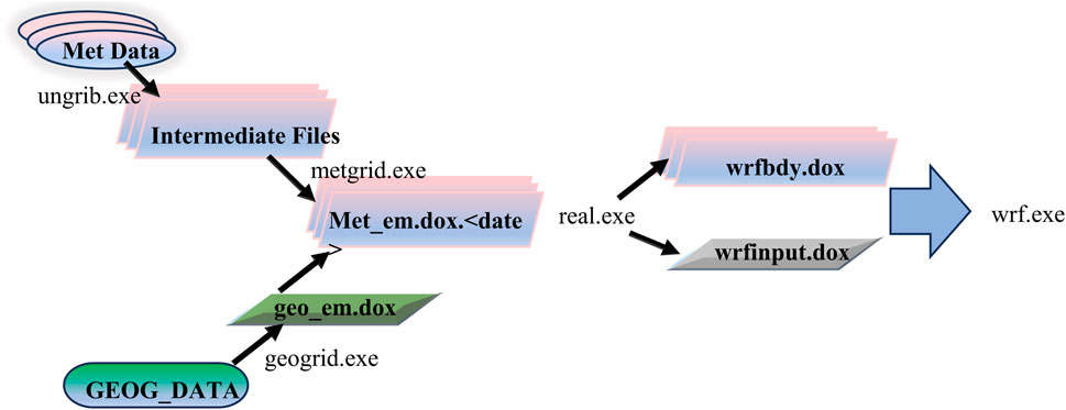
Figure 1. Meteorological data preprocessing.

The WRF-Chem model employed the following chemical and physical modules in this study: The RRTMG (Rapid Radiative Transfer Model for General Circulation Models) from a global atmospheric circulation model was selected to simulate longwave and shortwave radiation (Zhang et al., 2015). The cloud microphysics utilized the Morrison double-parameter scheme, and the cumulus convection parameterization employed the Kain-Fritsch scheme (Kain, 2004). Furthermore, the Noah land surface scheme (Jiménez and Dudhia, 2013) and the YSU planetary boundary layer (PBL) scheme (Hong et al., 2006) were chosen to specify the lower boundary conditions in the study. The chemical scheme employed was the CBM-Z gas-phase chemistry mechanism (Zaveri and Peters, 1999), along with the MOSAIC four-modal aerosol simulation mechanism (Zaveri et al., 2008). The Fast-J scheme was utilized for photochemistry (Wild et al., 2000).

The study region’s grid configuration was as follows: it comprised 24 vertical layers and featured two nested horizontal grids. The outer grid had a resolution of 36 km, while the inner grid had a resolution of 12 km. The second nested grid covered the entire regions of five provinces: Shandong, Zhejiang, Jiangsu, Henan, and Anhui. The regional center point was located at 36°N, 103.5°E. The anthropogenic emission source inventory was provided by Multi-resolution Emission Inventory model for Climate and air pollution research (MEIC group) in Tsinghua University, and the chemical boundary field was based on MOZART. The sources of biogenic emissions are obtained from the data downloaded from the National Center for Atmospheric Research (NCAR), accessible via the provided link (https://www.acom.ucar.edu/wrf-chem/download.shtml). This data is processed using the Model of Emissions of Gases and Aerosols from Nature (MEGAN) and its associated procedural framework. Due to limited computing resources, we selected autumn as the research period. During this season, the atmospheric conditions are relatively stable, which is unfavorable for the spread of pollutants.The simulation covered meteorological conditions from October 1st to 23 October 2022 and the output frequency of WRF-Chem is one simulation result per hour. To ensure the accuracy of results, a 1-week spin-up was conducted in the month prior to the research. Various meteorological parameter data were utilized for model evaluation, primarily including ground-level meteorological observation data such as humidity and visibility. This data was sourced from a global dataset provided by the National Center for Environmental Information (NCEI, https://www.ncei.noaa.gov/), encompassing essential meteorological data with quality control from relevant observation stations within the study area. Ground-based observation data for the particles are from the access of China National Environmental Monitoring Centre. The data includes hourly mass concentrations of PM_2.5, PM₁₀ and so on, providing a solid basis for evaluating model performance.

2.2 Extreme gradient boosting

XGBoost (Chen and Guestrin, 2016) is an efficient gradient boosting decision tree algorithm based on GBDT (Gradient Boosting Decision Trees). It minimizes the loss function through multiple iterations of multiple decision trees, continuously enhancing model accuracy using the “boosting” technique (Kim et al., 2022). This approach empowers XGBoost to excel in predictive and computational tasks across a variety of datasets. Furthermore, it can assess the significance of different input features in generating output data, facilitating an understanding of which features are pivotal for the model’s predictions. XGBoost is particularly well-suited for addressing regression and classification challenges (Phan et al., 2020). The XGBoost algorithm can be viewed as an additive model formed by the accumulation of ‘m’ regression trees, with the Formula 1 provided as follows:

${\widehat{y}}_i^m={\displaystyle \sum _{j=1}^m}{f}_j\left(x_i\right)(1)$

Let i represent the ith sample, X_i denote the features of the ith sample, and y_i be the prediction of this model for the ith sample. The revised content for the objective function (Equation 2) (Chen and Guestrin, 2016) is as follows:

$obj\left(\varphi \right)={\displaystyle \sum _{i=1}^n}L\left(y_i,{\widehat{y}}_i\right)+{\displaystyle \sum _{k=1}^m}\mathrm{\Omega }\left(f_k\right)(2)$

Where:

$\mathrm{\Omega }\left(f\right)=\gamma T+\frac{1}{2}\lambda {\displaystyle \sum _{j=1}^T}{\omega }_j^2$

Here, obj(φ) signifies the objective function, where φ represents the predictive function of the model. n represents the total number of samples in the dataset. L (y_i, ŷ_i) represents the loss function, which quantifies the difference between the predicted value ŷ_i for the ith sample and the true value $y_i$. And Ω(ƒ_k) serves as the regularization term, which is employed to control the complexity of the kth tree and mitigate the risk of overfitting. m denotes the total number of regression trees within the model. ω_j signifies the value assigned to the jth leaf node of a regression tree. T represents the number of current leaf nodes in the regression tree. The hyperparameters γ and λ are introduced to regulate the model’s complexity: γ is responsible for controlling the number of leaf nodes, while λ governs the sum of the squares of the leaf node weights. An increase in T corresponds to a deeper tree, which can lead to a greater propensity for overfitting. Consequently, the selection of these hyperparameters is essential for imposing an appropriate level of penalty on the model to enhance its generalization capabilities.

To compute visibility, we gathered data from the WRF-Chem model’s simulations, which included PM₁₀, PM_2.5, temperature (Ta), dew point temperature (Td), relative humidity (RH), atmospheric pressure (Pa), and wind speed (WS) as input for the XGBoost algorithm and we utilized existing visibility observation data to assess the accuracy of visibility calculations by XGBoost, following the methodology of previous research (Kim et al., 2022). In prior studies, when employing statistical methods like machine learning for prediction, it was common practice to select dry weather conditions with relative humidity below 60% to eliminate the effects of rapid aerosol hygroscopic growth under high humidity conditions (Robasky et al., 2006; Guo et al., 2020), with the aim of achieving a better model fit. However, in this study, the input data was obtained from WRF-Chem model simulations, which accurately represent meteorological elements after simulating the physical and chemical conditions of the atmosphere. Furthermore, the selected chemical option in this study allows some aqueous phases reacitons to take place, so that the complete feedback process of the aerosols can be accurately represented. Therefore, in this study, all data, except for invalid value, were employed to estimate visibility under all weather conditions.

The performance of the XGBoost model is notably influenced by parameter selection, with “max_depth” (the maximum depth of the binary tree) and “learning_rate” being key parameters. “max_depth” specifies the maximum length of the longest path from the root node to a leaf node in the decision tree. Its primary purpose is to limit the tree’s depth to prevent overfitting and excessive sensitivity to data details. On the other hand, “learning_rate” determines the extent of updates to the weights of leaf nodes in each iteration. It is used not only to control the training speed of the model but also to ensure model stability, enhance generalization performance, and reduce the risk of overfitting.

In this study, we randomly divided the data into training and testing sets in a 6:4 ratio. Through cross-validation, we systematically assessed the impact of various parameter combinations on the performance of the XGBoost model. Our analysis led us to determine the optimal parameter combination, which consisted of “max_depth = 7” and “learning_rate = 0.08,” ensuring that the model performs optimally when encountering unseen data.

2.3 Visibility parameterization equation

In this study, concerning the parameterization of visibility, we employed the most widely used Koschmieder equation (Israël et al., 1959) and the IMPROVE equation (Malm and Hand, 2007). The Koschmieder Equation 3 is as follows:

$V_R=\frac{K}{b_{ext}}(3)$

Where: V_R represents visibility (Km); K is a constant; b_ext denotes atmospheric extinction coefficient (Mm⁻¹).

This method has been improved, and the enhanced parameterization scheme takes into account the extinction coefficients of both particulate matter and gas molecules, including the scattering and absorption coefficients of gas molecules, for calculating atmospheric extinction coefficients (Hu et al., 2017).

$V_R=\frac{K}{b_p+b_{ag}+b_{sg}}\times {10}^6(4)$

In the Equation 4: V_R represents visibility in meters (m); K is a constant determined based on previous research approaches (Ozkaynak et al., 1985; Yu et al., 2016) b_sg stands for gas molecule scattering coefficient, primarily due to Rayleigh scattering by atmospheric molecules, which is typically assumed to be constant and has a value of 13 Mm⁻¹; b_p denotes the extinction coefficient of particulate matter, measured in Mm⁻¹; b_ag represents the absorption coefficient of gas molecules, primarily influenced by NO₂ pollution, with an absorption coefficient approximately 0.33 times the NO₂ mass concentration, measured in Mm⁻¹.

To simplify the calculation, an empirical formula based on the U.S. IMPROVE project was referenced (Sisler and Malm, 2000). The formula for the sum of particulate matter extinction coefficient and gas molecule absorption coefficient is as follows:

$\begin{array}{l}{b}_p+b_{ag}=2.2\times f_S\left(RH\right)\times S\left(sulfate\right)+4.8\times f_L\left(RH\right)\times L\left(sulfate\right)+2.4\times f_S\left(RH\right)\times S\left(nitrate\right)+\\ 5.1\times f_L\left(RH\right)\times L\left(nitrate\right)+2.8\times S\left(OM\right)+6.1\times L\left(OM\right)+10\times \left[EC\right]+\left[FS\right]+0.6\times \left[CM\right]+0.33\times \left[N{O}_2\right]\end{array}(5)$

In the Equation 5, f_S (RH) and f_L (RH) represent the hygroscopic growth factors for coarse and fine particles, respectively. These factors are functions of relative humidity (RH). L(X) and S(X) correspond to aerosol mass concentrations for coarse and fine particles, where X represents sulfate, nitrate, and organic matter [EC], [FS], and [CM] denote the concentrations of elemental carbon, fine soil dust aerosols, and coarse particles, measured in units of μg m⁻³. [NO₂] represents the volume fraction of NO₂, with units of 10⁻⁹.

2.4 Model evaluation methods

This study uses root mean square error (RMSE), mean deviation (MB), normalized mean deviation (NMB), and correlation coefficient (r) as indicators to evaluate model performance. The specific formula is as Equations 6–9 follows:

Root mean square error (RMSE):

$RMSE=\sqrt{\frac{1}{N}{\displaystyle \sum _{i=1}^N}{\left|f\left(x_i\right)-y_i\right|}^2}(6)$

Mean bias (MB):

$MB=\frac{{\displaystyle \sum _{i=1}^N}\left(f\left(x_i\right)-y_i\right)}{N}(7)$

Normalized mean bias (NMB):

$NMB=\frac{{\displaystyle \sum _{i=1}^N}\left(f\left(x_i\right)-y_i\right)}{{\displaystyle \sum _{i=1}^N}{y}_i}(8)$

Correlation coefficient (r):

$r=\frac{{\displaystyle \sum _{i=1}^N}\left(f\left({\mathrm{x}}_i\right)-\overline{f}\left(\mathrm{x}\right)\right)\left({\mathrm{y}}_i-\overline{y}\right)}{\sqrt{{\displaystyle \sum _{i=1}^N}{\left(f\left({\mathrm{x}}_i\right)-\overline{f}\left(\mathrm{x}\right)\right)}^2{\displaystyle \sum _{i=1}^N}{\left({\mathrm{y}}_i-\overline{y}\right)}^2}}(9)$

Where N represents the total number of samples, f (x_i) denotes the simulated visibility value computed for sample i, and y_i corresponds to the observed visibility value for sample i. A smaller RMSE or a larger r indicates better model performance.

3 Results and discussion

3.1 Visibility forecast model applicability verification

In this study, the WRF-Chem model is nested with d01 and d02 regions as illustrated in Figure 2.

Figure 2

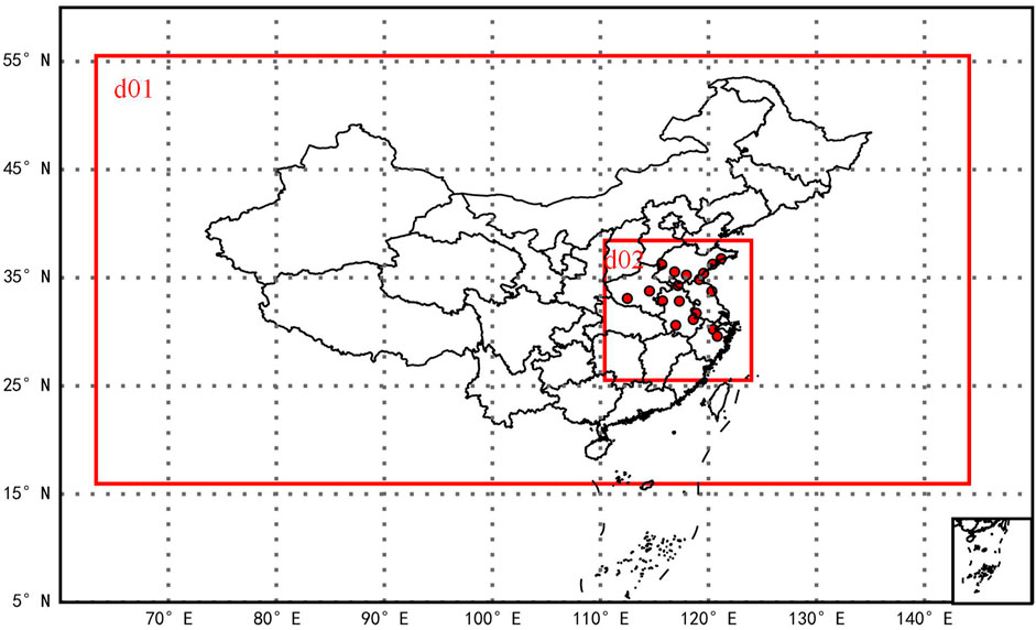
Figure 2. Schematic map of simulated domains in WRF-Chem and distribution of meteorological stations.

To ensure the reliability of the input features for the XGB and IMPROVE equations, it is imperative to comprehensively validate the accuracy of the WRF-Chem model, as shown in Table 1.

Table 1

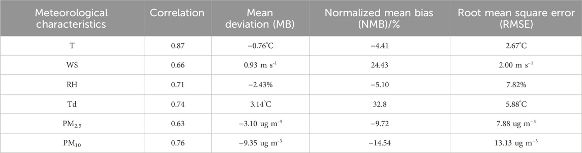
Table 1. Verification of meteorological element accuracy.

Table 1 reveals that the simulation results for temperature, wind speed, dew point temperature, relative humidity, and particulate matter all exhibit a high degree of accuracy, approaching or surpassing the levels of previously published studies (Tuccella et al., 2012; Zhou et al., 2017). The simulations of ground-level air temperature (T) at 2 m, wind speed at a height of 10 m (WS), relative humidity (RH) at 2 m among meteorological elements, and dew point temperature (Td) are satisfactory, with correlation coefficients of 0.87, 0.66, 0.71, and 0.74, respectively, which is comparatively well in relevant studies. The simulated temperature and relative humidity are both slightly underestimated, by 4.41% and 5.1% respectively, while the wind speed is overestimated less than 1 m/s. These discrepancies may stem from the complex interplay of various factors, including incomplete terrain information provided in the WRF preprocessing dataset, the spatial resolution of surface characteristics, and seasonal variations. These factors can lead to intricate temporal and spatial variations in the simulation of these meteorological factors, potentially resulting in biases in the simulation outcomes. Despite these noted deviations, the model, as a whole, maintains its credibility in replicating the meteorological conditions during the study period.

As for chemical species, ground-based measurement data of PM_2.5 mass concentration are provided for comparison with the simulation results. The concentration of fine particulate matter shows a reasonable agreement, with a correlation coefficient of 0.66, and a normalized mean bias of only −9.72%. Additionally, the correlation coefficient for PM₁₀ is 0.76, which is comparable to the simulation of PM_2.5 and also indicates an underestimation, with a bias of 14.54%. This suggests that the model can be able to offer valuable insights when simulating atmospheric conditions, particularly with respect to crucial meteorological factors such as temperature, relative humidity, dew point temperature, and particulate matter concentrations.

3.2 Analysis of XGBoost model results

The initial dataset is divided into a training set (60%) and a testing set (40%). 248 sets of samples are used for training, and 166 sets of samples are used for testing. This division is essential to prevent the model from becoming overly complex and tailored only to the training data, thus lacking the ability to make predictions for unknown data. The first portion of data (60%) is employed for model training. Through the use of features such as dew point temperature (Td), date, dew point deficit (Ta-Td), and various meteorological factors, the model progressively improves its predictive capabilities. By identifying and extracting general patterns within the dataset based on this series of input features, the model becomes proficient in making predictions for unknown data. Simultaneously, the second portion of data (40%) is reserved for testing the model’s performance on unfamiliar data. This phase aims to assess the model’s ability to generalize, evaluating how effectively the model predicts unknown data. This data splitting approach is crucial for a comprehensive evaluation of the model’s robustness, ensuring that the model can provide reliable predictions in practical applications.

To prevent the model from overfitting, we adopt an early stopping mechanism during the model training process to observe the performance of the model on the set in a timely manner. Meanwhile, to reduce the input of redundant information, the input features are screened and processed in advance. As indicated by Figure 3, the XGBoost (XGB) model’s loss curve exhibits a gradual reduction in variation during the training process, tending towards stability. This implies a continuous improvement in the model’s convergence, reducing its reliance on specific samples within the training data. To a large extent, the model has grasped the interrelationships among the data, which significantly impacts its performance on the test dataset. Furthermore, the descending trend of the loss curve suggests that the XGB model is likely to generalize better to unseen data, indicating improved stability and predictive capability when dealing with new data points.

Figure 3

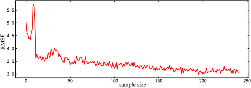
Figure 3. Loss curve of the training set.

To further validate the accuracy of XGBoost in calculating visibility, a correlation assessment was conducted between the computed XGB values and the actual observed results for the selected cities. The results, as depicted in Figure 4, reveal a strong positive correlation for the chosen cities, with the highest correlation reaching 0.98. The XGBoost model demonstrates an excellent correlation with observed visibility values, indicating its capability to accurately predict or compute visibility. The predictions closely align with the actual observed results, highlighting the model’s consistency and accuracy.

Figure 4

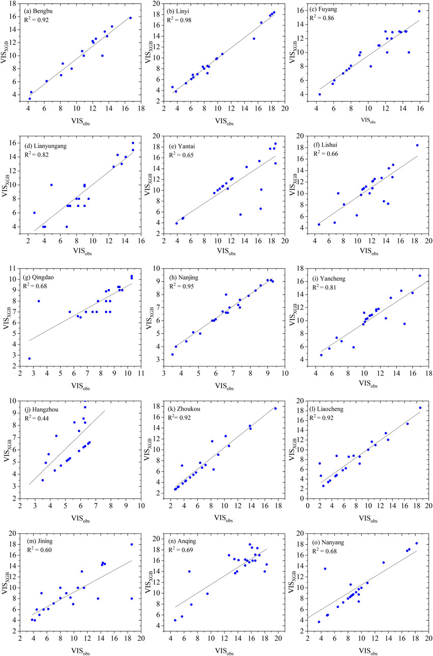
Figure 4. Verification of XGB simulation results for visibility [(A–O) are the cities studied].

Additionally, in the further analysis of the XGB model’s visibility simulation results, a spatial distribution map was created to visually assess the model’s performance across various geographical locations. Figure 5 vividly demonstrates the spatial performance of the XGB model in simulating visibility, along with its predictive accuracy and reliability in different cities. It is observed that the XGB model performs well over a broad geographical range, with the simulated mean visibility values closely matching the observed values. This indicates that the model not only excels in a specific city but also maintains a certain level of predictive accuracy in different geographical environments. In the investigated urban agglomeration, the model demonstrates relatively high prediction precision in five areas including Qingdao, Linyi, Lianyungang, Zhoukou and Nanjing. Even under the circumstances of unfavorable actual visibility conditions, the average error of visibility is less than 0.5 km.

Figure 5

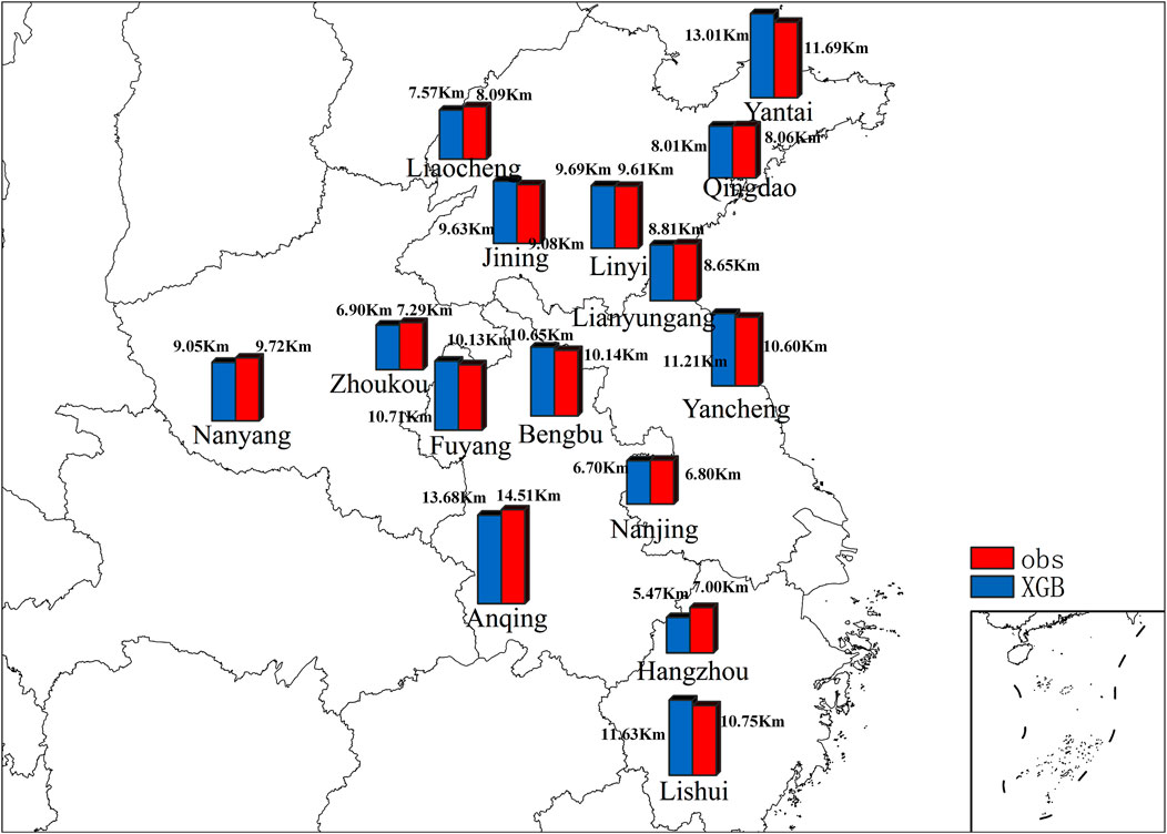
Figure 5. Spatial distribution map of XGB simulated mean visibility comparing with observation.

XGBoost calculates the importance scores for each input feature by considering the frequency of splitting and the gain from splitting. If a feature is used by multiple nodes, it significantly contributes to the model’s performance (Kim et al., 2022). To gain a visual and clear understanding of the impact of input variables on model performance, feature importance bar charts (as depicted in Figure 6) and correlation heatmaps (as shown in Figure 7) were generated. In previous research, relative humidity (RH) and aerosol substance mass concentrations (PM) have been identified as the two variables most closely associated with visibility (Kim et al., 2021; Feng et al., 2023; Zhang et al., 2019). In cities with more severe pollution, RH has a more pronounced influence on visibility trends. However, in cities with lower pollution levels, visibility trends are primarily affected by variations in particulate matter (Maurer et al., 2019). It's essential to note that when examining different regions and time frames, the relative importance of the same feature variables may vary. This variation is attributed to the changing influence of these variables in response to shifts in meteorological conditions. In this study, dew point temperature (Td) displayed the highest relative importance among all variables (40.95%), followed by the date sequence (date) with a relative importance of 9.45%, and dew point deficit (Ta-Td) with a relative importance of 8.53%. Due to the different seasons, meteorological parameters such as air pressure, humidity, temperature, and wind speed vary. For instance, in the winter, there is an increase in carbon emissions accompanied by phenomena like haze and snow. In contrast, the high temperatures and humidity during the summer lead to fog and rain. Therefore, both meteorological factors and pollutants exhibit temporal and spatial continuity. Analyzing historical date data is crucial for the model to recognize and establish specific weather patterns for given dates. This, in turn, helps the model consider seasonal variations and enhances prediction accuracy. Hence, the significance of the date feature in the XGBoost modeling process should not be underestimated.

Figure 6

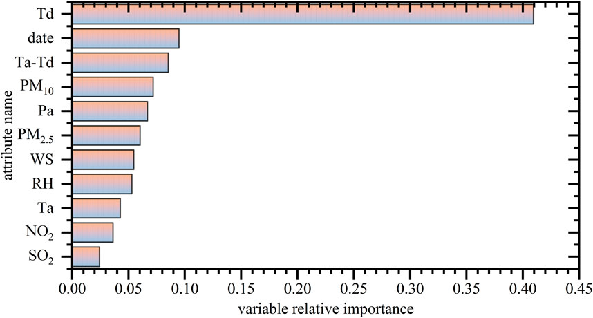
Figure 6. Bar chart of feature importance for XGB.

Figure 7

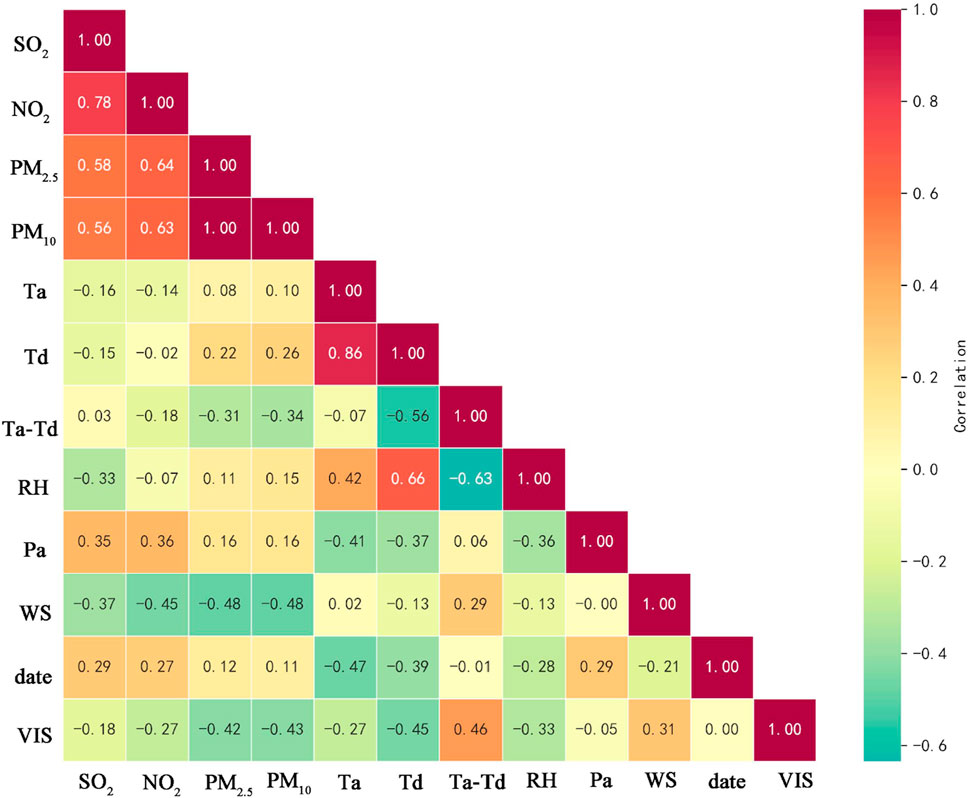
Figure 7. Correlation heatmap.

Figure 7 provides a clear visualization of the close relationships between various meteorological elements and visibility (VIS). Specifically, it illustrates the positive or negative impact of each element on visibility, contributing to a deeper understanding of how atmospheric conditions influence visibility. The analysis shows that pollutants have a negative impact on visibility, and they tend to mutually exacerbate each other’s growth, resulting in a detrimental effect on visibility. This implies that the presence of pollutants typically leads to decreased visibility. Furthermore, our study reveals that a larger dew point deficit (Ta-Td) has a positive effect on visibility. A larger dew point deficit indicates lower relative humidity in the atmosphere, often suggesting drier atmospheric conditions. In such dry atmospheric conditions, the hygroscopic formation of aerosols is unlikely to happen, so as fogs. This will contribute to the maintenance of good visibility.

As depicted in Figure 8, the RMSE of the forecasted visibility values, as modeled by the XGB algorithm, remains predominantly within the range of 3 Km. This indicates that the average discrepancy between the forecasted and the actual observed values is maintained at a relatively low level. The consistency of the RMSE, without significant fluctuations throughout the process, suggests that the XGB model is adept at discerning the interrelations among various input features from the data. Consequently, the forecasted values demonstrate a commendable degree of reliability.

Figure 8

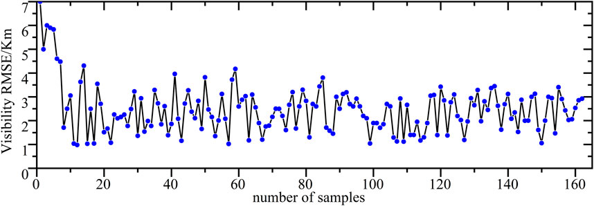
Figure 8. RMSE of the XGBoost-Modeled visibility values.

3.3 Visibility parameterization verification

To facilitate a better comparison with XGBoost (XGB), it is essential to validate the visibility results calculated based on the IMPROVE equation, as depicted in Figure 8. It is evident that in cities such as Bengbu (Figure 9A), Fuyang (Figure 9C), Lishui (Figure 9F), Jining (Figure 9M), Anqing (Figure 9N), and Nanyang (Figure 9O), the correlation is remarkably low, all below 0.4. This indicates a significant systematic bias in the visibility calculations by the IMPROVE equation. In contrast, XGB performs admirably in these cities, with correlations improving by 0.60, 0.56, 0.41, 0.24, 0.50, and 0.49, and achieving the best performance in Bengbu, where the correlation reaches 0.92. However, in the case of Lishui and Jining, XGB’s performance is relatively modest, with correlations of only 0.66 and 0.60, respectively.

Figure 9

Figure 9. Verification of IMPROVE simulation results for visibility [(A–O) are the cities studied].

Additionally, in the nine regions with favorable correlation results as illustrated in Figures 9B, D, E, and Figures 9G–L, the R² calculated using the IMPROVE equation range from 0.42 to 0.59. In these areas, the performance of XGB remains consistently stable. Notably, in the regions of Linyi (Figure 9B), Nanjing (Figures 9H), and Liaocheng (Figure 9I), the correlation of XGB has significantly improved, with increases of 0.54, 0.45, and 0.35, respectively. This suggests that XGB can provide a more reliable meteorological forecasting model.

3.4 Analysis of the visibility estimation results

In order to provide a clearer assessment of the validation performance for the IMPROVE equation and the XGBoost (XGB) model, we have computed their respective average simulated values, normalized mean biases (NMB), mean biases (MB), and root mean square errors (RMSE). As shown in Table 2, within the study area, the standardized mean bias for visibility calculated by the IMPROVE equation and the XGBoost model are 32.42% and −2.68%, respectively. The mean biases are 2.42 km and −0.07 km, respectively.

Table 2

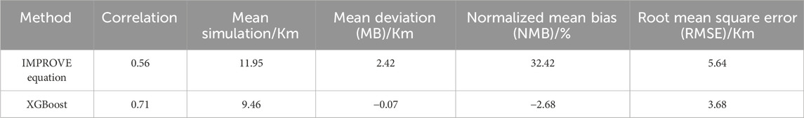
Table 2. Comparison and validation of improve and XGBoost.

This comparison reveals that, on the whole, the accuracy of the XGBoost model significantly surpasses that of the IMPROVE equation and is slightly lower than the actual observational values. Additionally, the root mean square error for the XGBoost model is 1.96 km smaller than that of the IMPROVE equation. This signifies that, relatively speaking, the XGBoost model demonstrates a smaller average error in relation to the actual observational values, further highlighting the superiority of the XGBoost model in predicting visibility.

From this analysis, it becomes evident that the XGBoost (XGB) model demonstrates a relatively high level of accuracy in simulating visibility. It is capable of modeling visibility based on input features and naturally adapts to the complex relationships within the data. Furthermore, the model possesses the ability to conduct importance analysis on the input data.

According to Figure 10, the results obtained by XGB closely align with the observed values, whereas the performance of the IMPROVE equation in simulating these aspects is subpar. This indicates that XGB excels in model training and data prediction, demonstrating significantly higher accuracy and better alignment with actual observations.

Figure 10

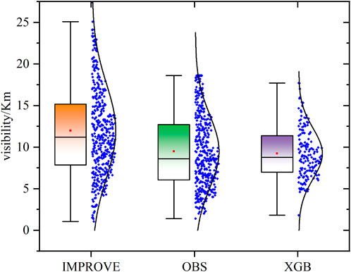
Figure 10. Assessing the performance of IMPROVE and XGB models through box plots.

Existing studies have demonstrated that particulate matter, relative humidity, and wind speed are significant factors influencing visibility variations (Qu et al., 2015; Lee et al., 2015; Kim et al., 2022). Especially under conditions of low visibility, there is a complex interplay among physical processes as well as chemical reactions, and a single mathematical equation is insufficient to accurately model the relationships between meteorological and chemical elements. As evidenced by the aforementioned validation, applying machine learning regression techniques to the outputs of numerical models can yield improved predictions of visibility. The gradient boosting algorithm constructs new decision trees, with each tree attempting to correct the errors of its predecessor, thereby capturing nonlinear characteristics within the data. In the XGBoost model, each tree is trained to address the predictive errors of the previous round of trees, constructing a series of functions that enhance the model’s generalization capabilities. This approach has shown excellent scalability and performance when dealing with large-scale datasets (Chen and Guestrin, 2016).

However, based on the comparative results presented in Table 2 and Figure 10, it is also noticeable that the XGB model’s simulation results tend to exhibit underestimation in comparison to the actual observed results. This underestimation can be influenced by multiple factors. Firstly, the performance of the XGB model heavily relies on the quality and accuracy of the input data. Despite the implementation of a series of advanced and comprehensive chemical reaction mechanisms in WRF-Chem to simulate the evolution of aerosols and chemical substances in the atmosphere, these mechanisms may still struggle to encompass all the intricate atmospheric chemical processes, particularly in extremely complex atmospheric conditions. As a result, the model may introduce errors in simulating atmospheric chemical reactions, leading to the observed biases between the observed and simulated values.

Secondly, the accuracy of emission sources within WRF-Chem also contributes to deviations in the simulation results. Errors in emission sources may further introduce inaccuracies when modeling visibility, thereby affecting the accuracy of the simulation results. Additionally, the complexity and uncertainty of atmospheric chemical reactions are also contributing factors to the underestimation. Atmospheric chemical processes involve numerous intricate reactions and interactions, and some of these processes may not be fully understood or adequately simulated. This lack of completeness implies that the model may fail to accurately capture all chemical changes in the atmosphere, resulting in the underestimation observed in the simulation results.

In contrast to the XGB model, the visibility calculated using the improve equation exhibits significant errors and lower confidence. Apart from the inherent reasons associated with WRF-Chem, this lower confidence may also be attributed to the improve equation itself. The improve equation is a relatively simple mathematical model that employs fixed parameters and is better suited for relatively restrained scenarios. In cases where the actual meteorological relationships are more complex, along with more sophisticated chemical feedback, certain important features may sometimes be overlooked, leading to substantial discrepancies between the improve equation’s predictions and the actual observed values.

4 Conclusion

In this study, we conducted an in-depth investigation of visibility in the East China region using simulated results from WRF-Chem for atmospheric pollutant concentrations and various meteorological elements in October. Visibility was calculated using both the XGBoost (XGB) model and the IMPROVE equation, and the simulation results were comprehensively assessed. Comparing the simulated visibility values with actual observations during the study period, it is evident that the XGB model demonstrates high accuracy and reliability in its predictions. The model exhibits adaptability to various regions and meteorological conditions, particularly in areas where the IMPROVE equation’s simulation performance is satisfying, the XGB model still showcases exceptional predictive capability.

What is particularly encouraging is that the XGBoost (XGB) model exhibits a significantly lower mean bias compared to the results obtained from the IMPROVE equation. This implies that the XGB model provides visibility simulations that are much closer to the actual observed values. Additionally, we observed a 0.15 improvement in the correlation with observational data when using the XGB model, further underscoring its exceptional performance. In summary, our research results strongly indicate that the XGB model offers higher accuracy, flexibility, and applicability in simulating visibility, especially in cases where the improve equation’s performance is less satisfactory. This finding holds significant implications for enhancing the accuracy of meteorological forecasts and environmental monitoring, providing robust support for future research and applications.

While this study highlights the crucial role of XGBoost (XGB) in post-processing WRF-Chem results, there are some noteworthy limitations in this study. Firstly, due to computational resource constraints and limitations in accessing relevant input data, WRF-Chem simulations were conducted for only 1 month. Future research could consider integrating WRF-Chem and XGB in different seasons and regions with varying background weather characteristics to comprehensively assess XGB’s performance. Secondly, this study does not fully explore and compare the uncertainties in natural and anthropogenic emission inventories. It is worth further investigation and research to effectively reduce biases in visibility prediction through improved emission inputs (Zhang et al., 2009). Finally, it is worth considering further improvements in other factors, such as terrain features and subgrid feedback loops in numerical simulations, in future research. These enhancements can significantly improve the accuracy of WRF-Chem simulation results and reduce biases in visibility prediction. Therefore, we encourage future research to focus more on these improvements to further enhance the accuracy of visibility simulations.

Data availability statement

The datasets presented in this study can be found in online repositories. The names of the repository/repositories and accession number(s) can be found in the article/supplementary material.

Author contributions

XZ: Supervision, Writing–original draft, Writing–review and editing, Formal Analysis, Funding acquisition. YW: Conceptualization, Methodology, Visualization, Writing–original draft, Writing–review and editing. ZZ: Supervision, Writing–review and editing. YL: Visualization, Writing–review and editing, Data curation. CY: Writing–review and editing, Visualization, Methodology. LS: Methodology, Writing–original draft. JS: Writing–review and editing, Supervision. P-WC: Supervision, Writing–review and editing, Formal Analysis.

Funding

The author(s) declare that financial support was received for the research, authorship, and/or publication of this article. This study is supported by the Natural Science Foundation of Tianjin of China (No. 23JCQNJC00190) and the Fundamental Research Funds for the Central Universities (No. 3122019066).

Conflict of interest

Author CY was employed by Harbin International Airport Co., Ltd.

The remaining authors declare that the research was conducted in the absence of any commercial or financial relationships that could be construed as a potential conflict of interest.

The author(s) declared that they were an editorial board member of Frontiers, at the time of submission. This had no impact on the peer review process and the final decision.

Generative AI statement

The author(s) declare that no Generative AI was used in the creation of this manuscript.

Publisher’s note

All claims expressed in this article are solely those of the authors and do not necessarily represent those of their affiliated organizations, or those of the publisher, the editors and the reviewers. Any product that may be evaluated in this article, or claim that may be made by its manufacturer, is not guaranteed or endorsed by the publisher.

References

Awad, M., Khanna, R., Awad, M., and Khanna, R. (2015). “Support vector regression,” in Efficient learning machines: theories, concepts, and applications for engineers and system designers, 67–80.

Google Scholar

Bari, D., and Ouagabi, A. J. S. A. S. (2020). Machine-learning regression applied to diagnose horizontal visibility from mesoscale NWP model forecasts. SN Appl. Sci. 2 (4), 556. doi:10.1007/s42452-020-2327-x

CrossRef Full Text | Google Scholar

Benjamin, S. G., Dévényi, D., Weygandt, S. S., Brundage, K. J., Brown, J. M., Grell, G. A., et al. (2004). An hourly assimilation–forecast cycle: the RUC. Mon. Weather Rev. 132 (2), 495–518. doi:10.1175/1520-0493(2004)132<0495:ahactr>2.0.co;2

CrossRef Full Text | Google Scholar

Castillo-Botón, C., Casillas-Pérez, D., Casanova-Mateo, C., Ghimire, S., Cerro-Prada, E., Gutierrez, P., et al. (2022). Machine learning regression and classification methods for fog events prediction. Atmos. Res. 272, 106157. doi:10.1016/j.atmosres.2022.106157

CrossRef Full Text | Google Scholar

Che, H., Xia, X., Zhao, H., Dubovik, O., Holben, B. N., Goloub, P., et al. (2019). Spatial distribution of aerosol microphysical and optical properties and direct radiative effect from the China Aerosol Remote Sensing Network. Atmos. Chem. Phys. 19 (18), 11843–11864. doi:10.5194/acp-19-11843-2019

CrossRef Full Text | Google Scholar

Che, H., Zhang, X., Li, Y., Zhou, Z., and Qu, J. (2007). Horizontal visibility trends in China 1981–2005. Geophys. Res. Lett. 34 (24). doi:10.1029/2007GL031450

CrossRef Full Text | Google Scholar

Chen, L., Liao, H., Li, K., Zhu, J., Long, Z., Yue, X., et al. (2023). Process-level quantification on opposite PM2. 5 changes during the COVID-19 lockdown over the north China plain. Environ. Sci. Technol. Lett. 10 (9), 779–785. doi:10.1021/acs.estlett.3c00490

CrossRef Full Text | Google Scholar

Chen, T., and Guestrin, C. (2016). Xgboost: a scalable tree boosting system. Proc. 22nd acm sigkdd Int. Conf. Knowl. Discov. data Min., 785–794. doi:10.1145/2939672.2939785

CrossRef Full Text | Google Scholar

Chmielecki, R. M., and Raftery, A. (2011). Probabilistic visibility forecasting using Bayesian model averaging. Mon. Weather Rev. 139 (5), 1626–1636. doi:10.1175/2010MWR3516.1

CrossRef Full Text | Google Scholar

Colabone, R., Ferrari, A. L., Vecchia, F., and Tech, A. (2015). Application of artificial neural networks for fog forecast. Management 7, 240–246. doi:10.5028/jatm.v7i2.446

CrossRef Full Text | Google Scholar

Cornejo-Bueno, L., Casanova-Mateo, C., Sanz-Justo, J., Cerro-Prada, E., and Salcedo-Sanz, S. (2017). Efficient prediction of low-visibility events at airports using machine-learning regression. Bound. Layer. Meteorol. 165 (2), 349–370. doi:10.1007/s10546-017-0276-8

CrossRef Full Text | Google Scholar

Deng, J., Wang, T., Jiang, Z., Xie, M., Zhang, R., Huang, X., et al. (2011). Characterization of visibility and its affecting factors over Nanjing, China. China 101 (3), 681–691. doi:10.1016/j.atmosres.2011.04.016

CrossRef Full Text | Google Scholar

Deng, J., Zhang, Y., Hong, Y., Xu, L., Chen, Y., Du, W., et al. (2016). Optical properties of PM2. 5 and the impacts of chemical compositions in the coastal city Xiamen in Chin. a 557, 665–675. doi:10.1016/j.scitotenv.2016.03.143

CrossRef Full Text | Google Scholar

Ding, A., Huang, X., Nie, W., Sun, J., Kerminen, V. M., Petäjä, T., et al. (2016). Enhanced haze pollution by black carbon in megacities in China. Geophys. Res. Lett. 43 (6), 2873–2879. doi:10.1002/2016GL067745

CrossRef Full Text | Google Scholar

Fang, Y., Wu, Y., Wu, F., Yan, Y., Liu, Q., Liu, N., et al. (2023). Short-term wind speed forecasting bias correction in the Hangzhou area of China based on a machine learning model. Atmospheric and Oceanic Science Letters, 16(4), 100339. doi:10.1016/j.aosl.2023.100339

CrossRef Full Text | Google Scholar

Feng, W., Wang, X., Shao, Z., Liao, H., Wang, Y., and Xie, M. (2023). Time-resolved measurements of PM_2.5 chemical composition and Brown carbon absorption in nanjing, East China: diurnal variations and organic tracer-based PMF analysis. based PMF Anal. 128, e2023JD039092. doi:10.1029/2023JD039092

CrossRef Full Text | Google Scholar

Gao, M., Carmichael, G. R., Wang, Y., Saide, P. E., Yu, M., Xin, J., et al. (2016). Modeling study of the 2010 regional haze event in the North China Plain. Atmos. Chem. Phys. 16 (3), 1673–1691. doi:10.5194/acp-16-1673-2016

CrossRef Full Text | Google Scholar

Gao, M., Han, Z., Tao, Z., Li, J., Kang, J. E., Huang, K., et al. (2020). Air quality and climate change, Topic 3 of the Model Inter-Comparison Study for Asia Phase III (MICS-Asia III) – Part 2: aerosol radiative effects and aerosol feedbacks. Atmos. Chem. Phys. 20 (2), 1147–1161. doi:10.5194/acp-20-1147-2020

CrossRef Full Text | Google Scholar

Gao, M., Saide, P. E., Xin, J., Wang, Y., Liu, Z., Wang, Y., et al. (2017). Estimates of health impacts and radiative forcing in winter haze in eastern China through constraints of surface PM_2.5 predictions. 5 Predict. 51 (4), 2178–2185. doi:10.1021/acs.est.6b03745

PubMed Abstract | CrossRef Full Text | Google Scholar

Gao, S., Lu, C., Zhu, J., Li, Y., Liu, Y., Zhao, B., et al. (2024). Using machine learning to predict cloud turbulent entrainment-mixing processes. J. Adv. Model. Earth Syst. 16, e2024MS004225. doi:10.1029/2024MS004225

CrossRef Full Text | Google Scholar

Gultepe, I., and Milbrandt, J. (2010). Probabilistic parameterizations of visibility using observations of rain precipitation rate, relative humidity, and visibility. Climatology, 49(1), 36–46. doi:10.1175/2009JAMC1927.1

CrossRef Full Text | Google Scholar

Guo, B., Wang, Y., Zhang, X., Che, H., Zhong, J., Chu, Y., et al. (2020). Temporal and spatial variations of haze and fog and the characteristics of PM2. 5 during heavy pollution episodes in China from 2013 to 2018. Atmos. Pollut. Res. 11 (10), 1847–1856. doi:10.1016/j.apr.2020.07.019

CrossRef Full Text | Google Scholar

Guo, J., Su, T., Li, Z., Miao, Y., Li, J., Liu, H., et al. (2017). Declining frequency of summertime local-scale precipitation over eastern China from 1970 to 2010 and its potential link to aerosols. Geophys. Res. Lett. 44 (11), 5700–5708. doi:10.1002/2017GL073533

CrossRef Full Text | Google Scholar

Hong, S.-Y., Noh, Y., and Dudhia, J. (2006). A new vertical diffusion package with an explicit treatment of entrainment processes. Mon. weather Rev. 134 (9), 2318–2341. doi:10.1175/MWR3199.1

CrossRef Full Text | Google Scholar

Hu, J., Zhao, T. L., and Zhang, Z. F. (2017). Upgradeding atmospheric visibility parameterization scheme for haze pollution environment. Res. Environ. Sci. 30 (11), 1680–1688. doi:10.13198/j.issn.1001-6929.2017.03.19

CrossRef Full Text | Google Scholar

Hu, W., Zhao, T., Bai, Y., Kong, S., Xiong, J., Sun, X., et al. (2021). Importance of regional PM2.5 transport and precipitation washout in heavy air pollution in the Twain-Hu Basin over Central China: observational analysis and WRF-Chem simulation. Chem. Simul. 758, 143710. doi:10.1016/j.scitotenv.2020.143710

PubMed Abstract | CrossRef Full Text | Google Scholar

Israël, H., Kasten, F., Israël, H., and Kasten, F. (1959). Koschmieders theorie der horizontalen sichtweite. VS Verlag für Sozialwissenschaften. 7–10.

Google Scholar

Jiménez, P. A., and Dudhia, J. (2013). On the ability of the WRF model to reproduce the surface wind direction over complex terrain. J. Appl. Meteorology Climatol. 52 (7), 1610–1617. doi:10.1175/JAMC-D-12-0266.1

CrossRef Full Text | Google Scholar

Kain, J. S. (2004). The Kain–Fritsch convective parameterization: an update. J. Appl. meteorology 43 (1), 170–181. doi:10.1175/1520-0450(2004)043<0170:TKCPAU>2.0.CO;2

CrossRef Full Text | Google Scholar

Kim, B.-Y., Cha, J. W., Chang, K.-H., and Lee, C. (2021). Visibility prediction over South Korea based on random forest. Atmos. (Basel). 12 (5), 552. doi:10.3390/atmos12050552

CrossRef Full Text | Google Scholar

Kim, B.-Y., Cha, J. W., Chang, K.-H., Lee, C. J. A., and Research, A. Q. (2022). Estimation of the visibility in Seoul, South Korea, based on particulate matter and weather data, using machine-learning algorithm. Aerosol Air Qual. Res. 22 (10), 220125. doi:10.4209/aaqr.220125

CrossRef Full Text | Google Scholar

Kim, B.-Y., Lim, Y.-K., and Cha, J. (2022). Short-term prediction of particulate matter (PM10 and PM2.5) in Seoul, South Korea using tree-based machine learning algorithms. South Korea using tree-based Mach. Learn. algorithms 13 (10), 101547. doi:10.1016/j.apr.2022.101547

CrossRef Full Text | Google Scholar

Kim, J., Kim, S. H., Seo, H. W., Wang, Y. V., and Lee, Y. G. (2022). Meteorological characteristics of fog events in Korean smart cities and machine learning based visibility estimation. Atmos. Res. 275, 106239. doi:10.1016/j.atmosres.2022.106239

CrossRef Full Text | Google Scholar

Kumar, B., Atey, K., Singh, B. B., Chattopadhyay, R., Acharya, N., Singh, M., et al. (2023). On the modern deep learning approaches for precipitation downscaling. Earth Sci. Inf. 16 (2), 1459–1472. doi:10.1007/s12145-023-00970-4

CrossRef Full Text | Google Scholar

Lee, J. Y., Jo, W. K., and Chun, H. H. (2015). Long-term trends in visibility and its relationship with mortality, air-quality index, and meteorological factors in selected areas of Korea. Aerosol Air Qual. Res. 15, 673–681. doi:10.4209/aaqr.2014.02.0036

CrossRef Full Text | Google Scholar

Liu, Y., Liu, S., Wang, Y., Lombardi, F., Han, J, and Systems, L. (2020). A survey of stochastic computing neural networks for machine learning applications. IEEE Trans. Neural Netw. Learn. Syst. 32 (7), 2809–2824. doi:10.1109/tnnls.2020.3009047

PubMed Abstract | CrossRef Full Text | Google Scholar

Malm, W. C., and Hand, J. (2007). An examination of the physical and optical properties of aerosols collected in the IMPROVE program. Atmos. Environ. X. 41 (16), 3407–3427. doi:10.1016/j.atmosenv.2006.12.012

CrossRef Full Text | Google Scholar

Maurer, M., Klemm, O., Lokys, H. L., Lin, N.-H. J. A., and Research, A. Q. (2019). Trends of fog and visibility in Taiwan: climate change or air quality improvement? Aerosol Air Qual. Res. 19 (4), 896–910. doi:10.4209/aaqr.2018.04.0152

CrossRef Full Text | Google Scholar

Ozkaynak, H., Schatz, A. D., Thurston, G. D., Isaacs, R. G., and Husar, R. (1985). Relationships between aerosol extinction coefficients derived from airport visual range observations and alternative measures of airborne particle mass. J. Air Pollut. Control Assoc. 35 (11), 1176–1185. doi:10.1080/00022470.1985.10466020

CrossRef Full Text | Google Scholar

Peng, Y., Wang, H., Hou, M., Jiang, T., Zhang, M., Zhao, T., et al. (2020). Improved method of visibility parameterization focusing on high humidity and aerosol concentrations during fog–haze events: application in the GRAPES_CAUCE model in Jing-Jin-Ji, China. China 222, 117139. doi:10.1016/j.atmosenv.2019.117139

CrossRef Full Text | Google Scholar

Peterson, L. E. J. S. (2009). K-nearest neighbor. Scholarpedia, 4(2), 1883. doi:10.4249/scholarpedia.1883

CrossRef Full Text | Google Scholar

Phan, Q.-T., Wu, Y.-K., and Phan, Q.-D. (2020). A comparative analysis of xgboost and temporal convolutional network models for wind power forecasting. 2020 Int. Symposium Comput. Consumer Control (IS3C), 416–419. doi:10.1109/IS3C50286.2020.00113

CrossRef Full Text | Google Scholar

Qu, W. J., Wang, J., Zhang, X. Y., and Sheng, L. F. (2015). Influence of relative humidity on aerosol composition: Impacts on light extinction and visibility impairment at two sites in coastal area. China. Atmos. Res. 153, 500–511. doi:10.1016/j.atmosres.2014.10.009

CrossRef Full Text | Google Scholar

Riedmiller, M. (1994). Advanced supervised learning in multi-layer perceptrons—from backpropagation to adaptive learning algorithms. Interfaces, 16(3), 265–278.

CrossRef Full Text | Google Scholar

Robasky, F. M., and Wilson, F. W. (2006). Statistical forecasting of ceiling for New York City airspace based on routine surface observations. 12th Conference on Aviation, Range, and Aerospace Meteorology. Atlanta, GA, Am. Meteor. Soc. Atlanta, GA.

Google Scholar

Roman Cascon, C., Steeneveld, G., Yagüe, C., Sastre, M., Arrillaga, J., and Maqueda, G. J. Q. (2016). Forecasting radiation fog at climatologically contrasting sites: evaluation of statistical methods and WRF. Quarterly journal of the royal meteorological society, 142(695), 1048–1063. doi:10.1002/qj.2708

CrossRef Full Text | Google Scholar

Sati, A. P., and Mohan, M. (2021). Impact of increase in urban sprawls representing five decades on summer-time air quality based on WRF-Chem model simulations over central-National Capital Region, India. India 12 (2), 404–416. doi:10.1016/j.apr.2020.12.002

CrossRef Full Text | Google Scholar

Shen, L., Fan, X., and Zhang, X. (2023). Analysis of temporal and spatial variation of visibility in Beijing, China, from 2015 to 2020. Natural Hazards Research, 3, 280, 285. doi:10.1016/j.nhres.2023.03.007

CrossRef Full Text | Google Scholar

Sisler, J. F., and Malm, W. C. (2000). Interpretation of trends of PM25 and reconstructed visibility from the IMPROVE network. J. Air and Waste Manag. Assoc. 50 (5), 775–789. doi:10.1080/10473289.2000.10464127

PubMed Abstract | CrossRef Full Text | Google Scholar

Steeneveld, G., Ronda, R., and Holtslag, A. (2015). The challenge of forecasting the onset and development of radiation fog using mesoscale atmospheric models. Bound. Layer. Meteorol. 154, 265–289. doi:10.1007/s10546-014-9973-8

CrossRef Full Text | Google Scholar

Tao, J., Zhang, L., Wu, Y., and Zhang, Z. J. A. E. (2020). Evaluation of the IMPROVE formulas based on Mie model in the calculation of particle scattering coefficient in an urban atmosphere. Atmos. Environ. X. 222, 117116. doi:10.1016/j.atmosenv.2019.117116

CrossRef Full Text | Google Scholar

Tuccella, P., Curci, G., Visconti, G., Bessagnet, B., Menut, L., and Park, R. (2012). Modeling of gas and aerosol with WRF/Chem over Europe: evaluation and sensitivity study. J. Geophys. Res. 117 (D3). doi:10.1029/2011JD016302

CrossRef Full Text | Google Scholar

Wang, H., Li, X., Shi, G., Cao, J., Li, C., Yang, F., et al. (2015). PM2. 5 chemical compositions and aerosol optical properties in Beijing during the late fall. Atmos. (Basel). 6 (2), 164–182. doi:10.3390/atmos6020164

CrossRef Full Text | Google Scholar

Wen, W., Li, L., Chan, P., Liu, Y.-Y., and Wei, M. J. A. (2023). Research on the usability of different machine learning methods in visibility forecasting. Atmosfera, 37. doi:10.20937/atm.53053

CrossRef Full Text | Google Scholar

Wild, O., Zhu, X., and Prather, M. J. (2000). Fast-J: accurate simulation of in-and below-cloud photolysis in tropospheric chemical models. J. Atmos. Chem. 37 (3), 245–282. doi:10.1023/A:1006415919030

CrossRef Full Text | Google Scholar

Xiong, X., Guo, X., Zeng, P., Zou, R., and Wang, X. (2022). A short-term wind power forecast method via xgboost hyper-parameters optimization. Front. Energy Res. 10, 905155. doi:10.3389/fenrg.2022.905155

CrossRef Full Text | Google Scholar

Yu, X., Ma, J., An, J., Yuan, L., Zhu, B., Liu, D., et al. (2016). Impacts of meteorological condition and aerosol chemical compositions on visibility impairment in Nanjing, China. China 131, 112–120. doi:10.1016/j.jclepro.2016.05.067

CrossRef Full Text | Google Scholar

Zaveri, R. A., Easter, R. C., Fast, J. D., and Peters, L. K. (2008). Model for simulating aerosol interactions and chemistry (MOSAIC). J. Geophys. Research-Atmospheres 113 (D13), 29. doi:10.1029/2007jd008782

CrossRef Full Text | Google Scholar

Zaveri, R. A., and Peters, L. K. (1999). A new lumped structure photochemical mechanism for large-scale applications. J. Geophys. Research-Atmospheres 104 (D23), 30387–30415. doi:10.1029/1999jd900876

CrossRef Full Text | Google Scholar

Zhang, B., Wang, Y., and Hao, J. (2015). Simulating aerosol–radiation–cloud feedbacks on meteorology and air quality over eastern China under severe haze conditionsin winter. Atmos. Chem. Phys. 15 (5), 2387–2404. doi:10.5194/acp-15-2387-2015

CrossRef Full Text | Google Scholar

Zhang, Q., Streets, D. G., Carmichael, G. R., He, K. B., Huo, H., Kannari, A., et al. (2009). Asian emissions in 2006 for the NASA INTEX-B mission. Atmos. Chem. Phys. 9 (14), 5131–5153. doi:10.5194/acp-9-5131-2009

CrossRef Full Text | Google Scholar

Zhang, Q., Zheng, Y., Tong, D., Shao, M., Wang, S., Zhang, Y., et al. (2019). Drivers of improved PM2. 5 air quality in China from 2013 to 2017. Proc. Natl. Acad. Sci. U. S. A. 116 (49), 24463–24469. doi:10.1073/pnas.1907956116

PubMed Abstract | CrossRef Full Text | Google Scholar

Zhang, Y., Wang, Y., Zhu, Y., Yang, L., Ge, L., and Luo, C. J. A. (2022). Visibility prediction based on machine learning algorithms. Atmos. (Basel). 13 (7), 1125. doi:10.3390/atmos13071125

CrossRef Full Text | Google Scholar

Zhou, G., Xu, J., Xie, Y., Chang, L., Gao, W., Gu, Y., et al. (2017). Numerical air quality forecasting over eastern China: an operational application of WRF-Chem. Chem 153, 94–108. doi:10.1016/j.atmosenv.2017.01.020

CrossRef Full Text | Google Scholar