Simulation of slope soil erosion intensity with different vegetation patterns based on cellular automata model

Introduction: Soil erosion plays a crucial role in soil and water conservation management, as well as in ecological construction planning. This study focuses on the slopes of three planting patterns (uniform distribution, aggregation distribution, and random distribution), along with bare slopes, in the Baojiagou watershed of the Pisha Sandstone area, based on soil erosion intensity grade maps after rainfall from 2021 to 2023.

Methods: A method combining Multi-Criteria Evaluation (MCE) and the CA-Markov model is used to analyze the spatial variation of soil erosion intensity types on different slopes. This approach integrates multiple influencing factors and generates a suitability map for the conversion of soil erosion intensity types. Ultimately, the dynamic characteristics of soil erosion in 2023 are simulated under various slope conditions.

Results: Results indicated: (1) The spatial distribution of simulated soil erosion intensity grade maps for different slopes largely aligned with actual maps, and regions with soil erosion depth greater than 3 cm were resistant to transitioning to lower erosion zones. (2) The Kappa coefficients for simulated soil erosion intensity in uniform distribution, random distribution, aggregate distribution, and bare control slopes were 65.24%, 73.62%, 75.88%, and 69.06%, respectively, confirming the feasibility of the CA-Markov model for simulating soil erosion dynamics. (3) The simulation of soil erosion intensity on different slopes in 2023 revealed that erosion intensity on uniformly distributed, aggregated, and bare control slopes remained predominantly in the erosion zone with a depth of 1–2 cm, while randomly distributed slopes experienced a shift from mild erosion area to slight erosion area.

Discussion: This study improves the understanding of soil erosion across different vegetation patterns and demonstrates the applicability of the CA-Markov model for simulating dynamic erosion on slopes. The findings contribute to the development of broader ecological models and offer insights into vegetation management and erosion control strategies for similar landscapes.

1 Introduction

Erosion is a continuous natural process occurring on the Earth’s surface, especially in arid and semi-arid regions (Zhang et al., 1996; Grazhdani and Shumka, 2007; Liu et al., 2016). Soil erosion depletes land resources, worsens ecological degradation, and threatens human survival and development (Nurlina et al., 2022; Porto et al., 2022). In the Pisha sandstone region of the Yellow River Basin, water and soil loss has led to desertification of one-third of fertile soil, severely impacting agriculture and the environment (Yeh et al., 2006; Liu and Zhang, 2015). Research has shown that vegetation plays a critical role in slope soil erosion, making it central to erosion control and watershed management (BriniImen et al., 2021). However, vegetation on slopes in this region often fails to provide sufficient coverage. More commonly, vegetation appears in patchy or strip patterns, resulting in a fragmented vegetation structure (Pajouhesh et al., 2020; Eigentler and Sherratt, 2020). This pattern of vegetation influences the redistribution of runoff and sediment during hydraulic erosion on slopes. Therefore, simulating soil erosion dynamics under the influence of vegetation patterns is essential.

With the advancement of quantitative analysis of vegetation pattern indices, combined with remote sensing and geographic information systems, various mathematical models have been applied to studying soil erosion and vegetation patterns. Among them, the cellular automata (CA) model effectively utilizes vegetation pattern characteristics to explain key processes influencing soil erosion (Xiang et al., 2019; Fazlolah et al., 2018; Zhang et al., 2017). CA (cellular automata), as a tool for studying complex spatial phenomena, offers excellent simulation capabilities and has been widely recognized in the geographic research community (Qun et al., 2019). Currently, many scholars have applied CA for spatio-temporal dynamic simulation and prediction of various geographical phenomena. For instance, Yuan et al. (2008) used the CA model to develop a small watershed erosion and sediment production process model, CASEM, and explored its application in simulating soil erosion processes. Ma et al. (2003) utilized the CA model, supported by GIS technology, to analyze the spatial evolution of soil erosion under different land-use models and predict erosion development trends based on various land-use plots. Chase Clement, 1992 developed a CA model to simulate rainfall spatter erosion and runoff on slopes using simple rules, achieving notable results. D'Ambrosio et al. (2001) developed SCAVATU, a CA-based model to simulate hydraulic soil erosion, and obtained favorable simulation results. Although the CA model has been successfully applied to simulate the spatial development of soil erosion in large watersheds, building a dynamic slope soil erosion model based on CA remains in the exploratory phase. Slope erosion, as a typical nonlinear dynamic system, involves highly complex internal development and evolutionary processes, characterized by significant uncertainty and chaos. Therefore, it is imperative to develop a slope soil erosion model capable of simulating complex spatio-temporal dynamics and the spatial evolution of erosion. The CA-Markov model, based on transition probability matrices and suitability maps, leverages CA’s spatial transformation capability to simulate complex systems and utilizes Markov’s strengths to predict future trends in soil erosion intensity. In CA-Markov model simulations, complex spatio-temporal processes and interactions occur between various erosion intensity levels, necessitating a simulation model for transforming different soil erosion intensities and expanding its application scope. Vegetation patterns regulate and redistribute runoff and sediment during slope hydraulic erosion (Crompton and Thompson, 2020). Thus, investigating the relationship between vegetation patterns and soil erosion at the slope scale is crucial for comprehensive soil and water conservation.

While much research has explored soil erosion in various contexts, few studies have focused on simulating slope erosion under different vegetation patch patterns. Unlike earlier models that predominantly consider uniform vegetation distributions, this study investigates the impact of varied vegetation patterns, such as random and aggregated distributions, on erosion dynamics. This approach provides a more nuanced understanding of the role of vegetation in regulating runoff and sediment flow, offering valuable insights for erosion control in challenging environments. Therefore, this study focuses on the slopes of three planting patterns (uniform distribution, random distribution, and aggregation distribution) and bare control slopes in the Baojiagou Watershed of the Pisha Sandstone area. Starting with the rainfall-soil-erosion relationship at the slope scale, field monitoring experiments were conducted using runoff plots under natural rainfall conditions. Based on soil erosion intensity maps of slopes with varying vegetation patterns over a 3-year rainfall period, the spatial variation and intensity of soil erosion types were analyzed across slopes with different vegetation patch patterns. The CA-Markov model in IDRISI software was used to examine the conversion rules of soil erosion intensity types, integrating various influencing factors. A suitability map for soil erosion intensity conversion was developed to simulate the dynamic characteristics of erosion on slopes with different vegetation patch patterns, further verifying the ecological benefits of vegetation and providing valuable references for soil and water conservation management in the Pisha sandstone region.

2 Research methodology and methods

2.1 Study area

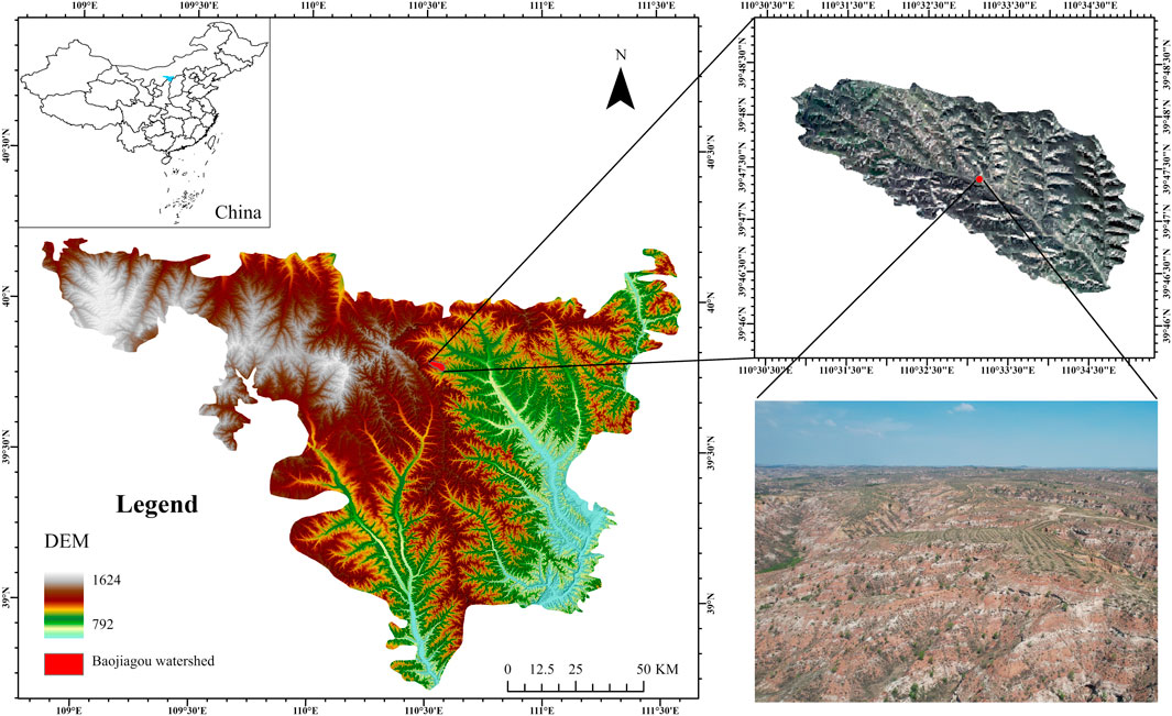
The study area is located in Nuanshui Town, Zhungeer Banner, Ordos City, Inner Mongolia (110°31′–110°35′E, 39°46′–39°48′N) (Figure 1). The elevation ranges from 1,145 to 1,330 m, with higher terrain in the north and lower in the south. The main zonal soil is chestnut-calcium soil, which has low organic matter content. The study area can be divided based on the type of surface cover and the degree of bedrock exposure into sand-covered sandstone areas, soil-covered sandstone areas, and exposed sandstone areas, with the exposed sandstone area having the harshest ecological environment. This area has a typical continental climate, with an average annual temperature of 6–9°C, a large diurnal temperature range, cold and dry winters with long seasons, and hot summers with short seasons. The average annual rainfall is 400 mm, and the rainfall is mainly concentrated in the summer (July-August). The average annual rainfall in summer is 256.4 mm, accounting for 64.1% of the total annual rainfall. Most of the rainfall is rainstorm (more than 50 mm), and the rainfall erosivity is high (489.87 MJ mm hm⁻² h⁻¹ a⁻¹). The frost-free period is 100–140 days, with abundant sunshine and an average annual wind speed of 2–4 m/s. The main vegetation includes Pinus tabuliformis Carr., Caragana korshinskii, Hippophae rhamnoides, Leymus chinensis, Salsola collina, as well as other psammophytes, swamp meadows, and degraded grasslands.

Figure 1

Figure 1. Location map of the study area.

2.2 Determination of vegetation pattern and plot layout

Based on ecological principles, three vegetation distribution patterns are identified: uniform, clustered, and random. Uniform distribution is typically observed in undisturbed wastelands, where vegetation is evenly spread across the surface. Random distribution patterns are often seen in areas with degraded surfaces or sparse vegetation. Clustered distribution is common in semi-arid or degraded ecosystems. These three vegetation patterns reflect the spatial distribution characteristics of vegetation within the study area. Due to the harsh ecological conditions, high rainfall intensity, and erosion-prone soils in the region, a comparison of these patterns reveals their differential impacts on soil and water conservation. When selecting sampling plots, it is ensured that the soil structure of the three types of plots is consistent, the vegetation species and coverage are similar, the slope gradient and aspect are the same, the slope length is greater than 20 m, and there is no human interference. At the same time, a slope with natural conditions identical to the research plots was selected, and all vegetation on the slope was removed to serve as a control plot (bare ground). After selecting the slope, adjacent 1 m × 1 m grid plots were delineated on the slope, for a total of 60 plots, and each plot was surveyed for plant community characteristics in sequence.

The study uses the variance-to-mean ratio method (Equations 1, 2) (Elias and Schindler, 2015) to determine the vegetation distribution patterns. This method is based on statistical principles and reveals the distribution characteristics of a sample by comparing the degree of dispersion (variance) of the data with its average level (mean). The ratio of variance to mean is relatively simple and can quickly identify and explain the distribution pattern of vegetation in a specific ecological environment. If S²/m = 0, it indicates a uniform distribution; If S²/m = 1, it indicates a random distribution; If S²/m is significantly greater than 1, it indicates an aggregated distribution (Table 1). The calculation formula is:

$\mathrm{M}={\displaystyle \sum _i^N}{M}_i/N(1)$

$S^2={\displaystyle \sum _i^N}{\left(M_i-\overline{M}\right)}^2/\left(N-1\right)(2)$

Table 1

Table 1. Vegetation distribution patterns determined by the variance-to-mean ratio method.

In the formula, N represents the number of basic plots, and M_i represents the number of individuals in the ith plot.

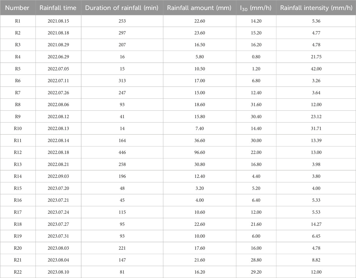
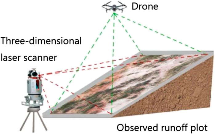
This experiment is a field runoff plot natural rainfall in-situ monitoring experiment, preparation began on 30 June 2021, and the observation period is the three rainy seasons (June-August) from 2021 to 2023. Based on the local topographic conditions, stainless steel plates were used to establish a runoff plot with dimensions of 10 m (length) × 2 m (width) on the slope (Figure 2). The plot boundaries are perpendicular to the contour lines and are driven 30 cm into the ground with a rubber mallet, leaving 20 cm above ground to block external runoff. The soil texture in the runoff plot is mainly composed of silt particles, accounting for 50.86%, followed by sand particles at 43.86%, and the smallest proportion is clay particles at 5.35%. A fixed rainfall monitoring point was set up next to the runoff plot, using a siphon-type automatic rain gauge to record atmospheric precipitation, and rain gauges were used for cross-validation to measure basic data such as rainfall amount, rainfall intensity, and duration of rainfall (Table 2).

Figure 2

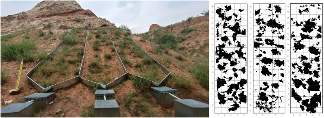
Figure 2. The layout of the runoff plot. Notes: In the figure, the vegetation patterns from left to right are uniform distribution, random distribution, and aggregated distribution.

Table 2

Table 2. Statistical table of rainfall characteristics.

2.3 Determination of soil erosion intensity

The Austrian-made RIGEL-400 3D laser scanner is used. This instrument uses a near-infrared laser beam with a rapid scanning mechanism to obtain 3D point cloud data and is characterized by high speed, non-contact, and high precision. The laser emission frequency is 300,000 bit/s, and the scanning accuracy (for a single 100 m measurement) is 3 mm (horizontal accuracy) × 2 mm (vertical accuracy). The instrument’s vertical scanning range is 270°, and the horizontal range is 360°. Scanning one slope takes about 1 min.

At both the bottom and top of each observed runoff plot, a fixed concrete stake is placed as a scanning station, and 5 to 8 fixed reference points are selected as stitching reference points for the scanned data of each station. Before the rainfall starts, an initial scan of the runoff plot is conducted to obtain the original slope point cloud data. After each rainfall, the slope is scanned again after the water has fully infiltrated, capturing the data on slope morphology changes. Before each scan, high-definition video equipment is used to record the process. The instrument is set up at the same position and tripod height for each scan, and reflective sample markers are placed along the plot boundaries to facilitate data trimming and overlay.

After completing data collection before and after rainfall, the “Camera” function of the 3D laser scanner is first used to inspect the scanned slope, ensuring that the surface is within the camera’s visible range and that the laser line’s visibility is optimized. Then, RiCAN PRO software is used to ensure that the input scan range allows the laser line’s intensity to fully pass through. The laser scan dataset is initially filtered through binarization, followed by point cloud registration and coordinate system transformation using the “Plane Surface Filter” and “Backsighting Orientation” functions in the software on the 668,431 scanned points. Since all data captured by the laser line are retained, there may still be non-terrain noise, such as vegetation, leading to a significant amount of redundant point cloud data. Therefore, further denoising and vegetation removal are performed using the “Filtering” and “Multi-Station Processing” functions in RiCAN PRO software, while controlling the standard deviation to ensure the quality of the point cloud data. After collecting elevation point cloud data from the slope, the point cloud data is converted into raster data using the “Data Conversion Module” in the ArcGIS software platform. Ultimately, an M-DEM with a resolution of 2 mm × 2 mm can be generated (Figure 3).

Figure 3

Figure 3. Schematic diagram of scanning runoff plot.

By subtracting the post-rainfall M-DEM from the pre-rainfall M-DEM, the difference can quantitatively describe the changes in the slope’s microtopography. In the ArcGIS spatial analysis module, spatial overlay analysis combined with the raster calculator is used to perform raster overlay subtraction and complete the calculation analysis. If the microtopography model after rainfall (M-DEM after) minus the microtopography model before erosion (M-DEM before) results in ∆M-DEM being negative, it indicates that the corresponding area is an erosion zone; if it is positive, it indicates that the corresponding area is a deposition zone. Specifically, erosion zone = (M-DEM_after)—(M-DEM_before) < 0; deposition zone = (M-DEM_after)—(M-DEM_before) > 0. Based on this calculation rule, the slope erosion intensity is classified according to the magnitude of ∆M-DEM.There are five levels of classification: >0 cm is a deposition zone; 0 to (−1) cm is slight erosion; (−1) to (−2) cm is mild erosion; (−2) to (−3) cm is moderate erosion; and <(−3) cm is severe erosion (Wan et al., 2022).

2.4 CA-Markov modeling method

CA-Markov modeling was performed using IDRISI Selva version 18.0. In the Markov model, the system’s state at a given time is only related to the previous state, and thus the Markov chain is realized by calculating the transition matrix of soil erosion intensity type changes over a certain period. This refers to the area of mutual conversion between soil erosion intensity types or the state transition probabilities (Zhang et al., 2021). The prediction formula for the probability of soil erosion intensity type changes is (Aguejdad, 2021):

$S_{t+1}=P_{ij}{S}_t(3)$

${\mathrm{S}}_{\mathrm{t}}$ and ${\mathrm{S}}_{\mathrm{t}+1}$ represent the soil erosion intensity types at time t and t + 1, respectively.

${\mathrm{P}}_{\text{ij}}$—the transfer probability matrix of soil erosion intensity types, i.e., the transfer probability of the soil erosion intensity type $\mathrm{i}$ to type $\mathrm{j}$.

P_ij was obtained by overlaying data from two consecutive periods. Since the time interval between the two datasets is difficult to control, the transition probabilities need to be adjusted to match the predicted time length, which works well when simulating relatively uniform spatial changes (Yi et al., 2021). However, soil erosion is intense and varies greatly across time scales. If time length is used to adjust the transition probabilities, it becomes difficult to reflect the characteristics of soil erosion, resulting in low accuracy in the simulation results. Soil erosion is caused by hydraulic erosion, with the primary hydraulic force coming from surface runoff scouring after rainfall. Therefore, rainfall plays a decisive role in soil erosion. Therefore, this study uses rainfall to adjust the transition probabilities, and the formula is as follows:

$P_{ij}^{\prime }=1-{\mathcal{l}}^{\frac{R^{\prime }}{R}In\left(1-P_{ij}\right)},i\ne j$

$P_{ij}^{\prime }=1-{\displaystyle \sum _{j=1}^{i\ne 1}}{P}_{ij}^{\prime },i=j(4)$

Where $P_{ij}^{\prime }$ stands for the transfer probability after transformation, (%); $R$ and $R^{\prime }$ denote the rainfall before and after transformation, respectively, (mm).

In Cellular Automata (CA), each variable only takes a finite number of states, and the rules governing state changes are local in both time and space (Zhang et al., 2023). Therefore, the CA model has strong spatial computing capabilities. The expression formula for the CA model is:

$S_{t+1}=f\left(A_t,N\right)(5)$

Where ${\mathrm{A}}_{\mathrm{t}}$ and ${\mathrm{A}}_{\mathrm{t}+1}$—finite and discrete state sets at time t and t + 1, respectively.

$\mathrm{N}$—size of cellular filter.

f —cellular transformation rule in local space.

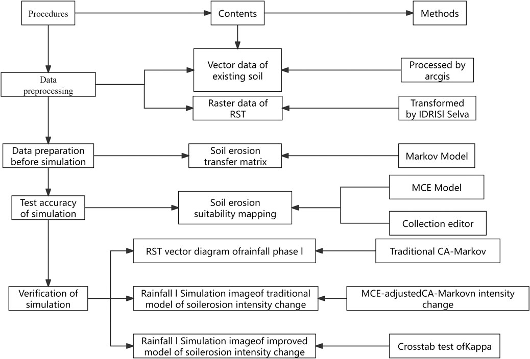
The CA-Markov model combines the features of two models, integrating them to complement each other’s strengths. It fully utilizes the powerful spatial simulation capabilities of the CA model and the long-term prediction ability of the Markov model. In this paper, the specific process of using the CA-Markov model to simulate and predict the spatial evolution of soil erosion intensity is as follows (Figure 4):

(1) Create a suitability map set. The paper sets the variation patterns between vegetation patterns and soil erosion intensity types as limiting factors based on the variation rules of soil erosion intensity types on slopes with different vegetation patterns. Slope, elevation, and the conditional probability images of various soil erosion intensity transfers are used as constraints, in combination with the influence of constraints and limiting factors on the transformation of soil erosion intensity types. Evolution rules or standards are defined based on the suitability map set generated by the MCE and COLLECTION EDIT modules, and the state of a cell at the next time step is determined based on the suitability map set.

(2) Define the size of the cells and construct a cell filter. The cell size is the same as the raster image size, and in this study, the raster size is set to 2 mm × 2 mm.

(3) Determine the starting time and the number of CA cycles. The post-rainfall slopes with different vegetation patterns from the first period are used as the initial data, and the number of CA cycles is set to 1. Combined with the soil erosion intensity transfer probability matrix for different periods, the suitability map set is obtained based on the transformation rules. This allows the simulation of soil erosion intensity grade maps for slopes with different vegetation patterns after the third period of rainfall.

Figure 4

Figure 4. Flowchart of the soil erosion intensity change simulation method.

2.5 Evaluation of simulation accuracy

The Kappa consistency test is a method for verifying the accuracy of model results. This coefficient is a commonly used indicator to measure the accuracy of predicted results (Cai and Wang, 2020), which allows the analysis of simulation results from both quantitative and spatial perspectives. The formula for calculating the validation accuracy of simulation results is as follows:

$kappa=\frac{P_0-P_e}{1-P_e}(6)$

Where Kappa—verification accuracy.

${\mathrm{p}}_{\mathrm{e}}{\mathrm{p}}_0$— overall simulation accuracy and theoretical simulation accuracy.

Kappa coefficient = 0-0.20 represents extremely low simulation accuracy; Kappa coefficient = 0.20–0.40 indicates ordinary simulation accuracy; Kappa coefficient = 0.40–0.60 denotes moderate simulation accuracy; Kappa coefficient = 0.60–0.80 stands for high simulation accuracy; Kappa coefficient = 0.80–1.00 reflects very high simulation accuracy.

2.6 Data processing

Statistical analysis of soil erosion intensity levels on slopes, under various vegetation patch patterns, was performed using ArcGIS 10.7.0.10450 software. Spatial overlay analysis of vegetation pattern and soil erosion intensity maps was conducted to determine the distribution of soil erosion in vegetation and non-vegetation areas on each slope. The classified micro-slope map and soil erosion intensity map were subsequently analyzed through spatial overlay to identify soil erosion distribution patterns at different slopes and reveal the micro-slope characteristics of soil erosion at varying gradients. Finally, the actual results were compared with the simulated data in ArcGIS to validate the accuracy of the simulated soil erosion intensity map under different vegetation patterns.

3 Results

3.1 Change analysis of slope soil erosion intensity

3.1.1 Analysis of area variation of soil erosion intensity on slope

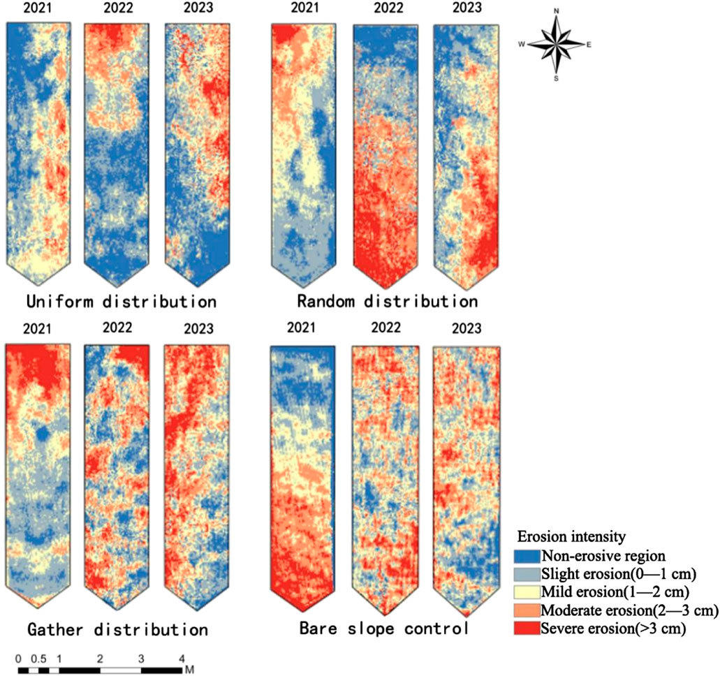
As shown in Figure 5, following erosion on slopes with varying vegetation patch patterns, the eroded area is larger than the deposition area.

Figure 5

Figure 5. Grade map of slope soil erosion intensity in 2021–2023.

As shown in Figure 6, on the uniformly distributed slope, the areas of the non-erosive zone and slight erosion area both show an upward trend. Slight erosion area saw the most significant increase, rising from 3.22 m² in 2011 to 3.76 m² in 2023, an increase of 0.54 m² or 3.10%. The areas of the mild erosion, moderate erosion, and severe erosion are all decreasing. On the randomly distributed slope, the areas of mild erosion and moderate erosion area both show an increasing trend. The moderate erosion area saw the most pronounced increase, rising from 3.08 m² in 2021 to 4.08 m² in 2023, an increase of 1.00 m² or 5.73%. However, the areas of the non-erosion zone, slight erosion area, and severe erosion area are all decreasing.

Figure 6

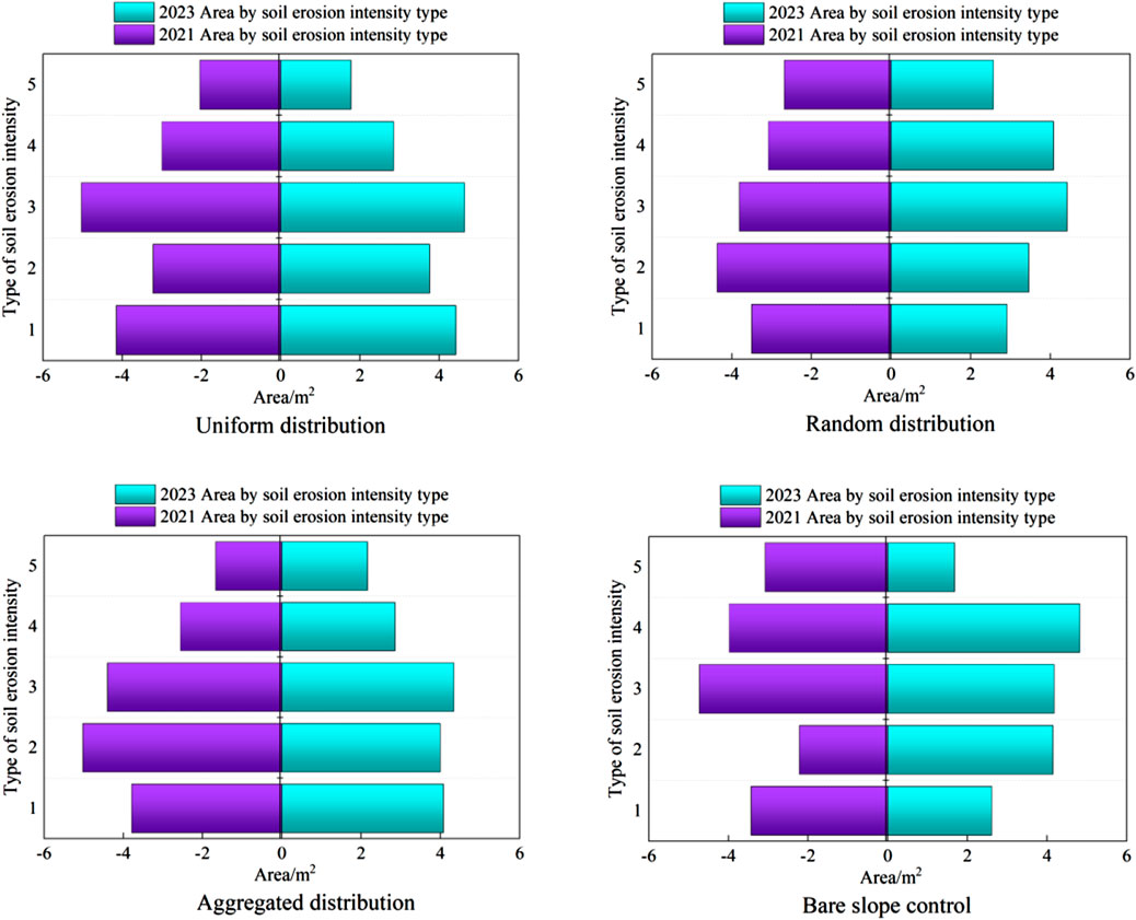
Figure 6. Area changes of soil erosion intensity on different slopes from 2021 to 2023. Note: 1, 2, 3, 4 and 5 are respectively non-erosive zones, slight erosion area, mild erosion area, moderate erosion area and severe erosion.

On the aggregate distribution slope, the areas of the non-erosive zone, moderate erosion area, and severe erosion area all exhibit an increasing trend. The severe erosion area saw the most significant growth, increasing from 1.67 m² in 2021 to 2.16 m² in 2023, an increase of 0.49 m² or 2.81%. However, the areas of the slight erosion and mild erosion are decreasing. On the bare slope control surface, the areas of the slight erosion and moderate erosion area both increased, with slight erosion area showing the most significant growth, rising from 2.22 m² in 2021 to 4.15 m² in 2023, an increase of 1.93 m² or 11.08%. However, the areas of the non-erosion zone, mild erosion area, and severe erosion area are all decreasing.

3.1.2 Analysis of the change of slope soil erosion intensity transfer direction

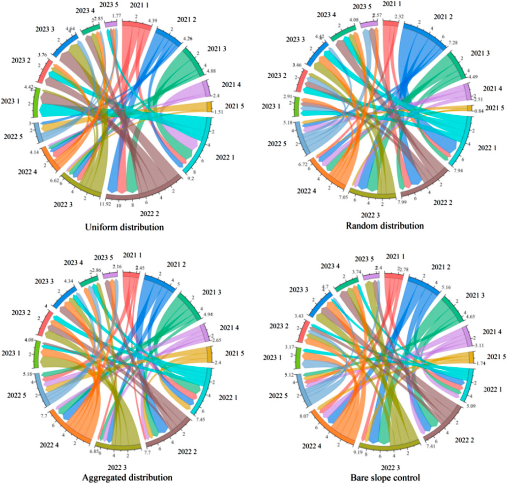
Figure 7 illustrates the changes in the transfer directions of soil erosion intensity on different slopes from 2021 to 2023. It provides a quantitative explanation of how the types of soil erosion intensity shift across slopes with varying vegetation patterns.

Figure 7

Figure 7. Transfer direction of soil erosion intensity.

As shown in Figure 7, on slopes with uniform vegetation distribution, the non-erosive zone and the mild erosion area can only transition to slight erosion area or moderate erosion area. Slight erosion area can transition to any other zone, whereas the moderate erosion area can only transition to the non-erosive or mild erosion area. The severe erosion area transitions solely to the mild erosion area.

On slopes with random vegetation distribution, the non-erosive zone and the severe erosion area can only transition to slight erosion area or moderate erosion area. mild erosion area can transition to any zone, while the mild erosion area transitions only to the non-erosive, slight erosion area, and moderate erosion area. The moderate erosion area can only transition to the mild erosion area and severe erosion area.

On slopes with aggregate vegetation distribution, the non-erosive zone can only transition to the mild erosion area, moderate erosion area, or severe erosion area. Slight erosion area transitions only to the non-erosive, mild erosion area, or moderate erosion area, whereas the mild erosion area can transition to any zone. The moderate erosion area and severe erosion area transition only to slight erosion area or mild erosion area.

On the bare slope control surface, the non-erosive zone, mild erosion area, and severe erosion area can transition to any other zone. Slight erosion area can transition only to the non-erosive, mild erosion area, or moderate erosion area, while the moderate erosion area can transition only to slight erosion area, mild erosion area, or severe erosion area.

3.2 Analysis of influencing factors of slope soil erosion intensity

3.2.1 Superposition analysis of vegetation pattern and soil erosion intensity

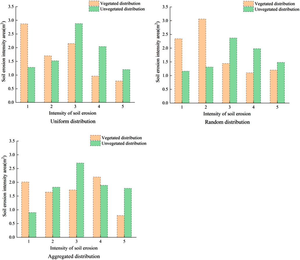
Vegetation patterns can effectively impede sediment movement, thereby influencing slope soil erosion. Based on the vegetation distribution characteristics of each slope, areas are classified into vegetated and non-vegetated zones, and the patterns and characteristics of soil erosion in these zones are analyzed. As shown in Figure 8, on the uniformly distributed slope, the non-erosive zone and slight erosion area have the largest areas within the vegetated zone, measuring 2.87 m² and 3.01 m², respectively. The mild erosion area, moderate erosion area, and severe erosion area are largest in the non-vegetated area, at 2.88 m², 1.79 m², and 3.04 m², respectively. On the randomly distributed slope, the non-erosive zone and slight erosion area have the largest areas in the vegetated region (2.87 m², 3.01 m²), while the mild erosion area, moderate erosion area, and severe erosion area are largest in the non-vegetated region (2.88 m², 1.79 m², 3.04 m²). On the aggregate distribution slope, the non-erosive zone and the moderate erosion area have the largest areas in the vegetated region (2.87 m², 3.01 m²). Slight erosion area, mild erosion area, and severe erosion area are largest in the non-vegetated region (2.88 m², 1.79 m², 3.04 m²).

Figure 8

Figure 8. Soil erosion distribution in vegetated and non-vegetated areas.

3.2.2 Superposition analysis of micro-slope and soil erosion intensity

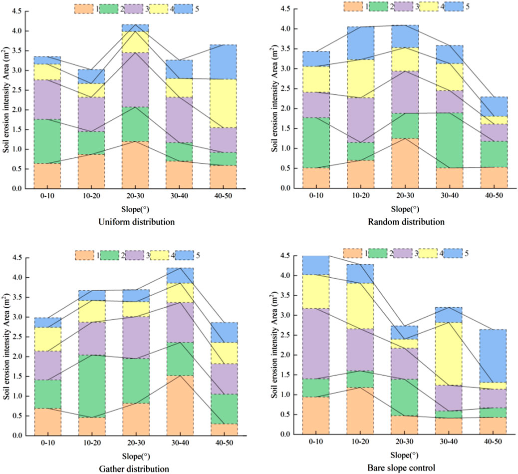
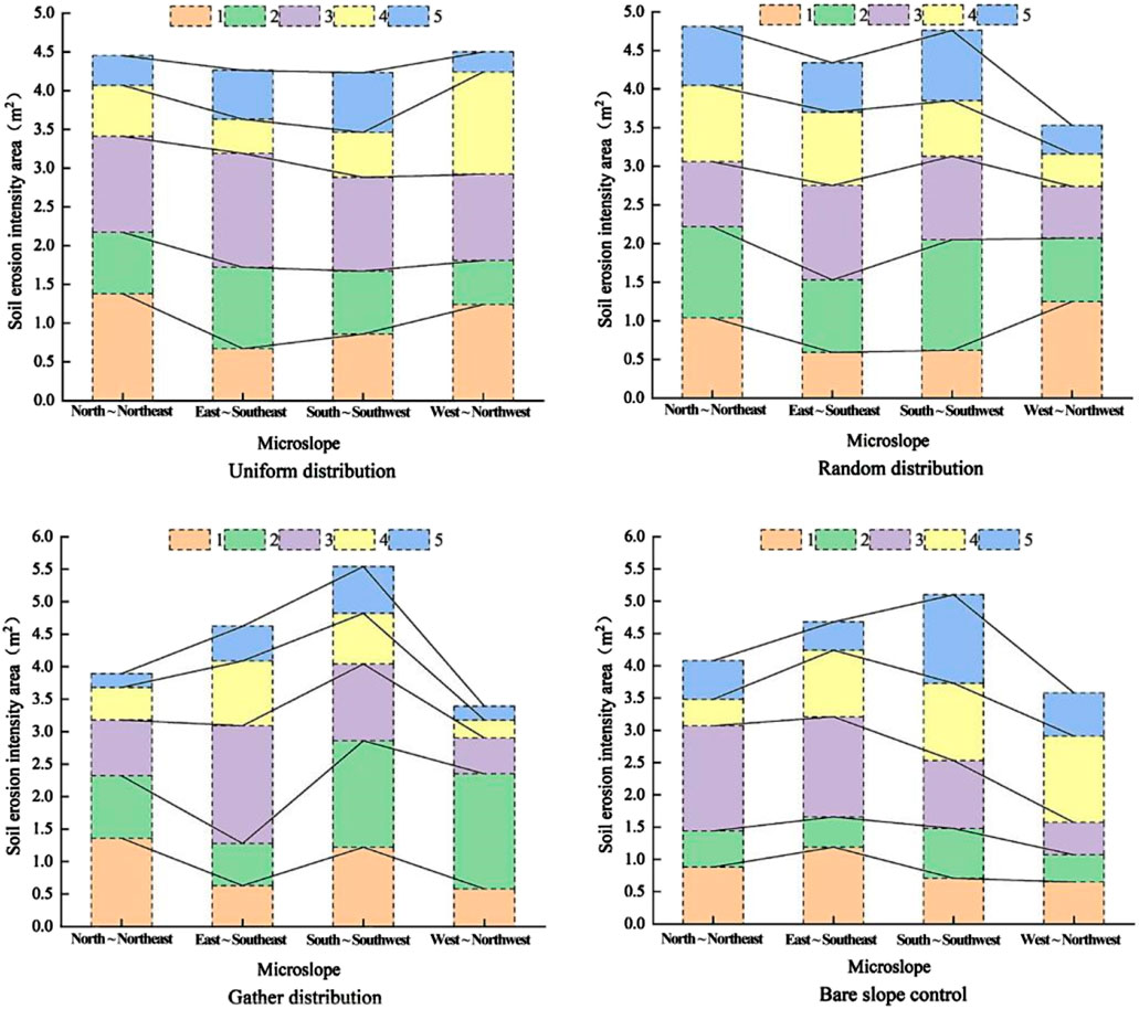
As shown in Figure 9, on the uniformly distributed slope, the largest areas of the non-erosive zone, slight erosion area, mild erosion area, moderate erosion area, and severe erosion area occur on micro-slopes of 20°–30°, 0°–10°, 20°–30°, 40°–50°, and 40°–50°, respectively, with areas of 1.20 m², 1.12 m², 1.38 m², 1.23 m², and 0.87 m². On the randomly distributed slope, the largest areas of the non-erosive zone, slight erosion area, mild erosion area, moderate erosion area, and severe erosion area are found on micro-slopes of 20°–30°, 30°–40°, 10°–20°, 10°–20°, and 30°–40°, respectively, with areas of 1.25 m², 1.38 m², 1.12 m², 0.96 m², and 0.82 m². On the aggregate distribution slope, the largest areas of the non-erosive zone, slight erosion area, mild erosion area, moderate erosion area, and severe erosion area are found on micro-slopes of 30°–40°, 10°–20°, 20°–30°, 0°–10°, and 40°–50°, respectively, with areas of 1.52 m², 1.58 m², 1.06 m², 0.60 m², and 0.50 m². On the bare slope control surface, the largest areas of the non-erosive zone, slight erosion area, mild erosion area, moderate erosion area, and severe erosion area are on micro-slopes of 10°–20°, 20°–30°, 0°–10°, 30°–40°, and 40°–50°, respectively, with areas of 1.18 m², 0.92 m², 1.77 m², 1.58 m², and 1.33 m².

Figure 9

Figure 9. Micro slope characteristics of soil erosion distribution.

3.2.3 Superposition analysis of micro-slope direction and soil erosion intensity

The micro-slope directions were reclassified into four ranges: north to northeast (337.5°–22.5°), east to southeast (22.5°–67.5°), south to southwest (157.5°–202.5°), and west to northwest (247.5°–337.5°). As shown in Figure 10, on the uniformly distributed slope, the largest upward distribution areas of the non-erosive zone, slight erosion area, mild erosion area, moderate erosion area, and severe erosion area are found in the north-northeast, east-southeast, east-southeast, west-northwest, and south-southwest, respectively, with areas of 1.38 m², 1.05 m², 1.47 m², 1.32 m², and 0.77 m². On the randomly distributed slope, the largest upward distribution areas of the non-erosive zone, slight erosion area, mild erosion area, moderate erosion area, and severe erosion area are found in the west-northwest, south-southwest, east-southeast, north-northeast, and south-southwest, respectively, with areas of 1.25 m², 1.43 m², 1.22 m², 0.99 m², and 0.91 m². On the aggregate distribution slope, the largest upward distribution areas of the non-erosive zone, slight erosion area, mild erosion area, moderate erosion area, and severe erosion area are found in the north-northeast, west-northwest, east-southeast, east-southeast, and south-southwest, respectively, with areas of 1.36 m², 1.77 m², 1.81 m², 1.00 m², and 0.72 m². On the bare slope control surface, the largest areas of the non-erosive zone, slight erosion area, mild erosion area, moderate erosion area, and severe erosion area are found in the east-southeast, south-southwest, north-northeast, west-northwest, and south-southwest, respectively, with areas of 1.19 m², 0.77 m², 1.63 m², 1.34 m², and 1.37 m².

Figure 10

Figure 10. Micro-slope characteristics of soil erosion distribution.

3.3 Simulation and precision inspection of slope soil erosion intensity

3.3.1 Markov transfer probability matrix

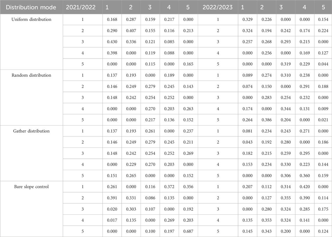
In this study, rainfall is very important as an indicator of the corrected transfer probability. The rainfall corresponding to the 3-year soil erosion data (29 August 2021–10 August 2023) was recorded by a siphon self-counting rain gauge. Firstly, the transfer probability matrix of 29 August 2021 and 3 September 2022 is calculated, and the conversion is carried out according to the rainfall during this period and the rainfall from 3 September 2022 to 10 August 2023. The transfer probability matrix for 29 August 2021 and 3 September 2022 is converted into the transfer probability matrix for 3 September 2022–10 August 2023, as shown in Table 3 (Equations 3, 4).

Table 3

Table 3. Type transfer probability matrix of slope soil erosion on slopes (m²).

3.3.2 Analysis of suitability rules of slope soil erosion intensity types

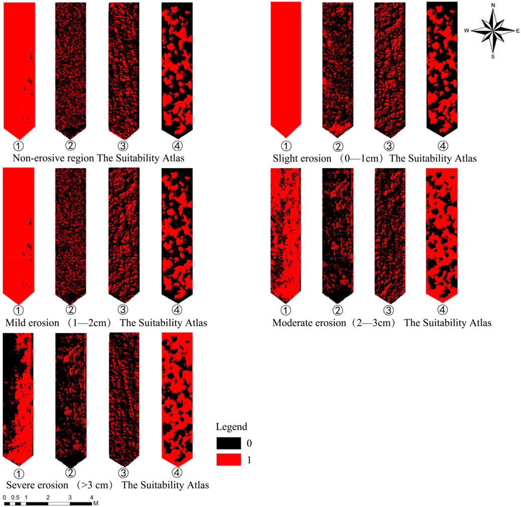
Soil erosion intensity types, vegetation distribution areas, micro-slope, and micro-aspect are key factors that influence the soil erosion process. These factors interact according to specific rules and mechanisms, determining both the intensity and spatial distribution of soil erosion in different regions. When formulating suitability rules, it is important to consider the protective effect of different vegetation types and distribution patterns on areas with varying erosion intensities. Erosion intensity types are classified according to slope steepness, while changes in micro-slope lead to variations in local erosion intensity. Micro-aspect, referring to the orientation of the slope surface, directly affects water flow direction, sunlight exposure, and rainfall distribution. Therefore, variations in micro-aspect must also be considered when developing soil erosion intensity suitability rules. Therefore, these factors are treated as constraints, and to ensure objectivity in evaluation, Boolean mapping (where areas outside the scope of consideration are assigned a value of 0, and areas to be considered are assigned a value of 1) is employed in MCE (Multi-Criteria Evaluation). For each type of soil erosion intensity, locations where transformation is not possible are set to 0, while those where transformation is possible are set to 1. This process involves analyzing the suitability rules for soil erosion intensity on different slopes and generating suitability maps for different soil erosion intensity types (Figure 11). Taking the uniform distribution of vegetation pattern as an example:

 (1) Rules for the conversion of non-erosive zones.

  ① Limitations: Restrict conversion to >3 cm erosive zones (0 for >3 cm, 1 for others).

  ② The area with a slight slope of 20°–30° is designated as a suitable development area for non-erosion areas (1 for this range, 0 otherwise).

  ③ The area with a micro-slope direction of north to northeast is designated as a suitable development area of non-erosion area (1 for these directions, 0 otherwise).

  ④ The area with vegetation distribution is designated as a non-erosion area suitable for development (1 for vegetated, 0 otherwise).

 (2) Rule of 0–1 cm erosion zone (slight erosion area) conversion.

  ① Conversion Flexibility: No restrictions on conversion (all zones set to 1).

  ② The area with a slight slope of 0°–10° is designated as the suitable development area of the erosion area of 0–1 cm (1 within this range, 0 otherwise).

  ③ The area with micro-slope direction from east to southeast is designated as the suitable development area of slight erosion area (1 within this range, 0 otherwise).

  ④ The area with vegetation distribution is designated as the suitable development area of slight erosion area (1 within this range, 0 otherwise).

 (3) Conversion rules of 1–2 cm erosion zone (mild erosion area).

  ① Limitations: Restrict conversion to >3 cm zones (0 for >3 cm, 1 for others).

  ② The area with a slope of 20°–30° is designated as a suitable development area of mild erosion area (1 within this range, 0 otherwise).

  ③ The area with micro-slope direction from east to southeast is designated as the suitable development area of mild erosion area (1 within this range, 0 otherwise).

  ④ The vegetation distribution area is designated as the suitable development area of mild erosion area (1 within this range, 0 otherwise).

 (4) Conversion rules of 2–3 cm erosion zone (moderate erosion area).

  ① Limitations: Restrict conversion to slight erosion area and >3 cm zones (0 for these, 1 for others).

  ② The area with a slight slope of 40°–50° is designated as a suitable development area of moderate erosion area (1 within this range, 0 otherwise).

  ③ The area with micro-slope direction from west to northwest is designated as the suitable development area of moderate erosion area (1 within this range, 0 otherwise).

  ④ The non-vegetation distribution area is designated as the suitable development area of moderate erosion area (1 within this range, 0 otherwise).

(5) >3 cm erosion zone (severe erosion area) conversion rules.

  ① Limitations: Restrict conversion to non-erosion, slight erosion area, and moderate erosion area (0 for these, 1 for others).

  ② The area with a slight slope of 40°–50° is designated as the suitable development area of the erosion area of >3 cm (1 within this range, 0 otherwise).

  ③ The area with a micro-slope direction of south to southwest is designated as the suitable development area of the erosion area of >3 cm (1 within this range, 0 otherwise).

  ④ The non-vegetation distribution area is designated as the suitable development area of the erosion area of >3 cm (1 within this range, 0 otherwise).

Figure 11

Figure 11. Suitability atlas of evenly distributed soil erosion intensity types.

3.3.3 Simulation of slope soil erosion intensity

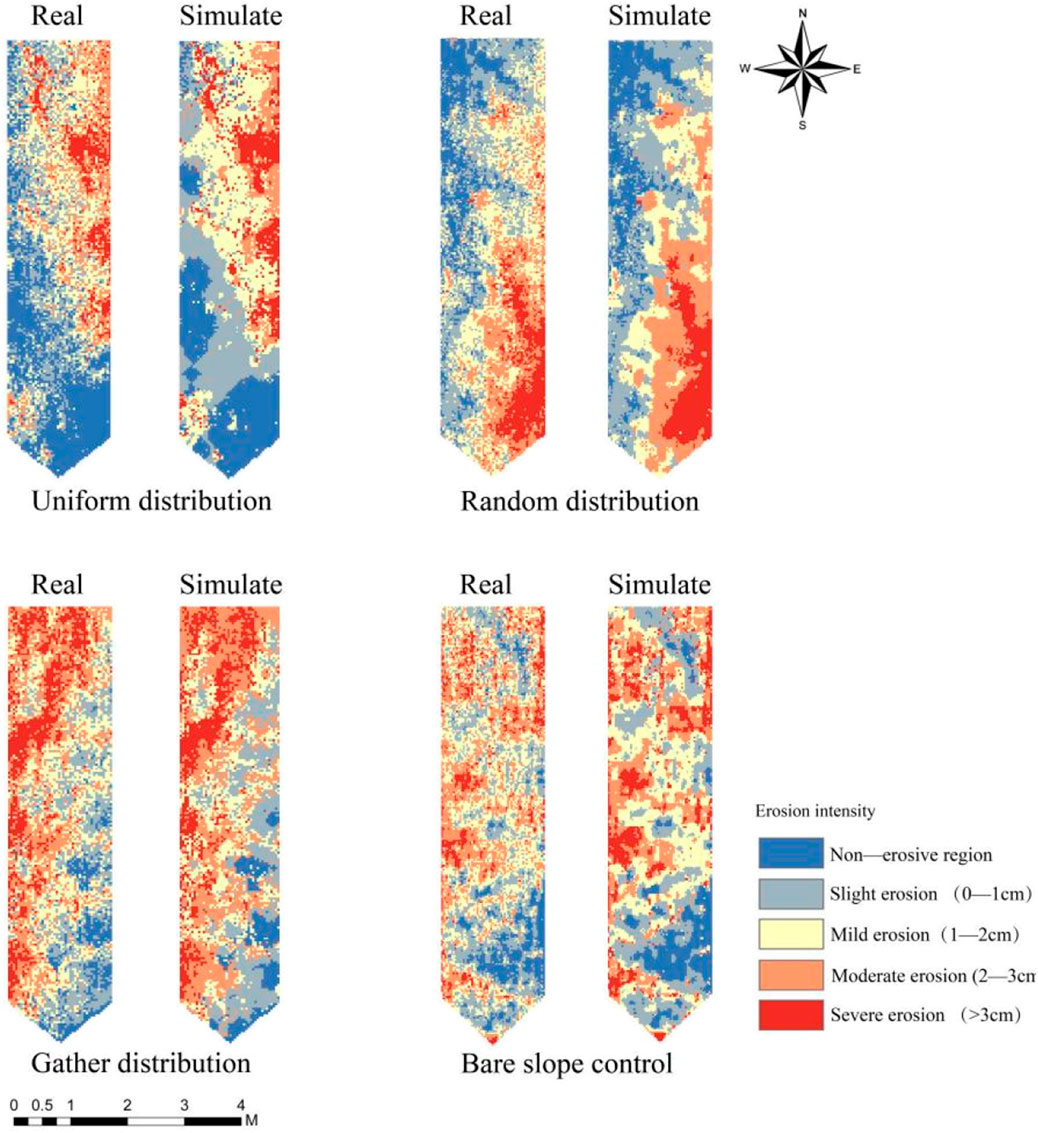
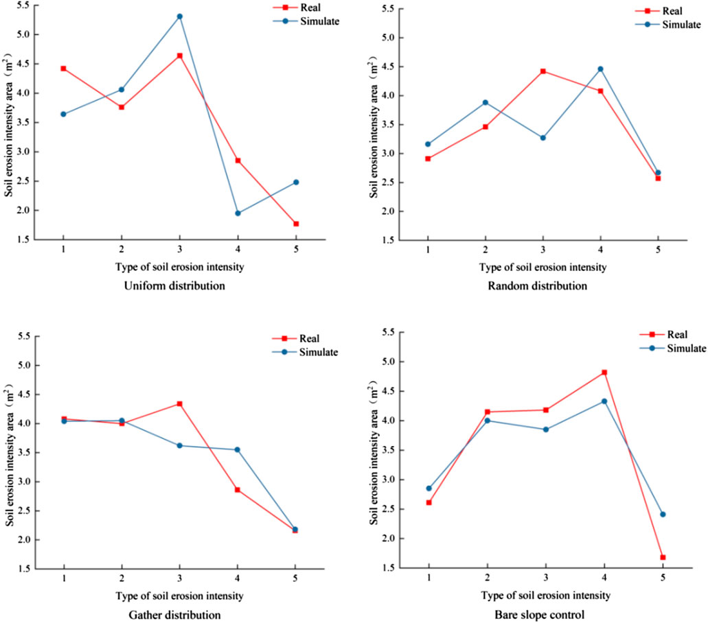
Based on the data preparation outlined above, the simulation of the 2023 soil erosion intensity grade charts for different slopes was conducted, with the resulting charts displayed in Figure 12 (Equation 5). As shown in Figure 12, the spatial layout of the actual soil erosion intensity grade diagram generally aligns with that of the simulated diagram. The uniformly distributed slope remains dominated by the mild erosion area, while the randomly distributed slope primarily transitions from the mild erosion area to the moderate erosion area. The aggregate slope shifted from the mild erosion area to slight erosion area, while the bare slope continues to be dominated by the moderate erosion area.

Figure 12

Figure 12. Simulation of soil erosion intensity levels.

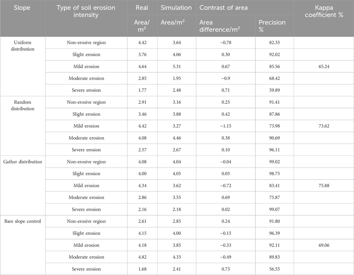
The simulated results were further compared with the actual areas of soil erosion intensity types (Figure 13). As shown in Figure 13, on the uniformly distributed slope, the simulated areas of slight erosion area, mild erosion area, and severe erosion area all increased, with the severe erosion area showing the largest increase (0.71 m²). Conversely, the areas of the non-erosive zone and moderate erosion area decreased, with the moderate erosion area experiencing the most significant decrease (0.9 m²). On the randomly distributed slope, the simulated areas of the non-erosive zone, slight erosion area, moderate erosion area, and severe erosion area all increased, with the moderate erosion area showing the greatest increase (0.42 m²). Meanwhile, the area of the mild erosion area decreased by 1.15 m². On the aggregate distribution slope, the simulated areas of slight erosion area, moderate erosion area, and severe erosion area all increased, with the moderate erosion area experiencing the largest increase (0.69 m²). In contrast, the areas of the non-erosive zone and the mild erosion area both decreased significantly (0.72 m²). On the bare slope control surface, the simulated areas of the non-erosive zone and severe erosion area increased, with the severe erosion area showing the greatest increase (0.73 m²). In contrast, the areas of slight erosion, mild erosion area, and moderate erosion area zone decreased, with the moderate erosion area experiencing the largest decrease (0.49 m²).

Figure 13

Figure 13. Comparison of simulated area of soil erosion intensity.

3.3.4 Simulation accuracy test

The soil erosion intensity grade map of different slopes in 2023 was simulated, and the accuracy of the simulation was tested by using the measured data of soil erosion intensity of different slopes in 2023. As shown in Table 4, the Kappa coefficients for soil erosion intensity simulation (Equation 6) on the uniformly distributed slope, randomly distributed slope, aggregate distributed slope, and control slope were 65.24%, 73.62%, 75.88%, and 69.06%, respectively. These values indicate a good fit and suggest that the simulated data effectively represents the mutual transformation trends among various types. This indicates that the model can predict future changes in soil erosion intensity.

Table 4

Table 4. Simulation and accuracy test of slope soil erosion intensity on slopes.

The accuracy of slight erosion area is high at 92.02%, while the accuracies of the moderate erosion area and severe erosion area are lower at 68.42% and 59.89%, respectively. The simulation accuracies for the non-erosive zone, moderate erosion area, and severe erosion area were higher, reaching 91.41%, 90.69%, and 96.11%, respectively. In contrast, the accuracies of slight erosion area and mild erosion area are lower, at 87.86% and 73.98%, respectively. The simulation accuracies for the non-erosive zone, slight erosion area, and severe erosion area are notably high, reaching 99.02%, 98.75%, and 99.07%, respectively. In contrast, the accuracies of the mild erosion area and moderate erosion area are lower, at 83.41% and 75.87%, respectively. The simulation accuracies for the non-erosive zone, slight erosion area, mild erosion area, and moderate erosion area are higher than those for the bare slope, reaching 91.8%, 96.39%, 92.11%, and 89.83%, respectively. Conversely, the accuracy of the severe erosion area is lower, at only 56.55%.

4 Discussion

4.1 Applicability of MCE-CA-Markov model

Slope is a fundamental component of soil erosion control and research within a basin or region. The occurrence, development, and evolution of soil erosion on slopes are complex phenomena, with vegetation being the primary factor influencing the erosion process. However, current research on soil erosion on slopes with vegetation patterns primarily focuses on post-event control measures. Relatively few studies have been conducted on simulating soil erosion on slopes with vegetation patch patterns (Chen, 2006). Typically, soil erosion intensity is simulated using the RUSLE equation as a variable. He et al. (2014) analyzed the soil erosion status of three experimental plots and two control plots under three rainfall conditions, applying the CA-Markov method to simulate soil erosion across five plots (Sun and Deng, 2015). The results were very close to the observed outcomes. This approach not only offers a novel idea and method for simulating slope soil erosion but also serves as a reference for vegetation management in controlling slope erosion.

The CA-Markov model is empirical, predicting changes in the subsequent period based on prior changes. This model treats the simulated ecological process as uniform, with rainfall serving as the primary driving force for soil erosion, which varies significantly over time. Consequently, this study employs a method to fit the characteristics of runoff, sediment yield, and rainfall for different slopes. The results indicated that rainfall, runoff, and sediment yield had the most significant effects. Therefore, rainfall was chosen to replace the time step in the modified transfer probability matrix (Ji et al., 2019), and the multi-criteria evaluation method in IDRISI was utilized to integrate various influencing factors, completing the simulation of the spatial evolution of soil erosion intensity changes across different vegetation patch patterns on slopes.

The Kappa coefficients for the simulated maps of soil erosion intensity for uniform distribution, random distribution, aggregate distribution, and bare slope control were 65.24%, 73.62%, 75.88%, and 69.06%, respectively. These results demonstrate that the MCE-CA-Markov model is effective for simulating the evolution of soil erosion, with high simulation accuracy. However, when simulating slopes under 3 years of erosion conditions, the model assumes that the effects of slope length and soil erodibility (K value) are uniform across all slopes. It only considers several factors, including rainfall, soil transformation status, vegetation patch patterns, micro-slope, and micro-slope orientation. Among these factors, soil transformation status pertains to the transfer of various soil erosion intensity types. Internal transfers are frequent, and the vegetation patch pattern, micro-slope, and micro-slope direction interact with soil erosion intensity to establish rules based on the most suitable areas for each type of soil erosion intensity. Consequently, the naming rules are somewhat subjective, introducing a degree of instability into the simulation. This leads to relatively large errors in the simulation results of the CA-Markov model (Sun and Deng, 2015).

Since simulation research on slope soil erosion is still in an exploratory phase, some theoretical methods remain underdeveloped. The Pisha sandstone area is characterized by unique eroded soil and semi-arid climate, providing a unique test site. However, due to differences in soil erodibility, cohesion and hydraulic properties, the performance of the model in other environments (e.g., wet, clay-rich soils or dry sandy land) may vary. For example, in areas with high clay content, the soil is not easily moved by rainfall immediately, but may experience slow and continuous erosion under saturated conditions. Integrating soil composition factors (such as clay and organic matter content) in the model can improve adaptability and enable more accurate erosion simulation in different landscapes. To address these shortcomings, the author plans to use MCE to spatialize additional data and integrate it into conversion rules for creating suitability maps in future research. Adjusting the cell size to the most appropriate grid dimension could significantly enhance the accuracy of the simulation (Zhao et al., 2013).

4.2 Difference analysis of simulation accuracy of soil erosion intensity on slopes

The simulation revealed that the erosion area of severe erosion increased the most on both the uniformly distributed slope (0.71 m²) and the bare control slope (0.73 m²). In contrast, the simulated erosion area of moderate erosion increased the most on the randomly distributed slope (0.42 m²) and the aggregated distributed slope (0.69 m²). Generally, the simulated areas of different slopes show the most significant increase in the >2 cm erosion zone. This trend occurs because, during model simulation, as rainfall causes erosion, the model tends to simulate a transformation from lower to higher erosion zones. Consequently, the simulated area of the higher erosion zone is much greater than the actual area.

The results indicate significant differences in the simulation precision of soil erosion intensity across different slopes. In comparison to other slopes, the Kappa coefficient for the soil erosion intensity grade simulation map of uniformly distributed slopes is relatively low at 65.24%. This is attributed to the more frequent internal transfers occurring on uniformly distributed slopes during the third phase of rainfall (Nikolaos et al., 2020). This introduces some instability into the simulation, leading to reduced accuracy in the simulated soil erosion intensity grade map. Table 4 shows that the simulation accuracies for slight erosion area on uniformly distributed, randomly distributed, clustered distributed, and bare control slopes are 92.02%, 87.86%, 98.7 5%, and 96.39%, respectively. Overall, the simulation accuracy of slight erosion area across different slopes is generally high. This is because slight erosion area represents a low-intensity erosion zone, which typically does not transform into a lower intensity zone after erosion (Mohamed et al., 2021). As a result, it remains relatively stable, whereas other zones can simultaneously transform into erosion zones with varying degrees of intensity after different erosion levels, leading to scattered cellular state changes and added uncertainties. Consequently, its interaction with other erosion areas is more complex, resulting in lower simulation accuracy.

In addition to the factors considered in the model, there may be other influences. The accuracy of the model may be affected by root structure, as plants with deeper roots can significantly reduce erosion, even on slopes with minimal vegetation coverage (Feng et al., 2018; Yu et al., 2019). Further investigation into root density and structure as anti-erosion factors could improve the model, particularly in areas with more variable root systems, such as aggregated and random vegetation patterns. Moreover, the Pisha sandstone region exhibits complex soil dynamics, influenced by the composition of sand and silt, which vary in their resistance to erosion. Incorporating soil composition parameters, such as clay content or organic matter, may enhance the accuracy of simulations for areas with high erosion intensity (Rodrigo-Comino et al., 2018; Gong et al., 2023). In conclusion, although the MCE-CA-Markov model successfully simulates erosion trends for different slope types, addressing the aforementioned factors could improve the accuracy of predictions for high-erosion intensity areas and provide a more detailed understanding of soil erosion dynamics under varying environmental conditions. Future research could integrate these factors to provide a more comprehensive erosion simulation framework, applicable to complex landscapes such as the Pisha sandstone region.

4.3 Effects of vegetation patch pattern on soil erosion on slope

The patch pattern of vegetation has a significant impact on the soil erosion process on slopes. Different vegetation distribution patterns regulate soil erosion by altering the flow paths of water and the movement of sediments. In this study, soil erosion intensity is lower on slopes with uniformly distributed vegetation patches. This may be due to the changes in the hydrological connectivity of the slope surface. The uniform distribution pattern is more evenly distributed and more dispersed than the aggregated and random distribution patterns. The hydrological connectivity of vegetation in this pattern is the weakest, meaning that the uniform distribution of vegetation fragments the slope more, making it easier for water and sediment flow to be intercepted by vegetation patches (Tang et al., 2021). As a result (Figure 5), the effective space for erosion on the slope is reduced, leading to increased soil accumulation. This results in a higher soil infiltration rate and a significant reduction in runoff and sediment production during the erosion process. This effectively reduces the transport of coarse sediments and obstructs the direct flow paths of water. In contrast, vegetation patches in random distribution are more likely to form irregular flow channels, leading to increased erosion intensity in localized areas. During heavy rainfall, water flow converges between randomly distributed vegetation patches, resulting in uneven distribution of erosion patches and potentially forming localized areas of high erosion intensity (Huang et al., 2017). Compared to the previous two vegetation patterns, aggregated vegetation communities typically consist of larger patches. These larger patches increase water retention time and promote downward water infiltration, thereby reducing erosion rates. Therefore, aggregated vegetation patches effectively trap larger particles, reducing the downslope movement of sediments (Zhao et al., 2020; Liu et al., 2018). Consequently, this characteristic makes the optimized layout of aggregated distribution highly significant for the practical application of soil and water conservation.

Additionally, this study found that after rainfall, the terrain factors on uniformly distributed slopes showed the smallest changes, while the bare slope control surface showed the greatest changes in micro-topographic factors. However, regardless of the vegetation patch pattern, individual plants, clusters, or patches of vegetation on the upslope direction will form raised soil mounds that intercept soil. Due to the different spatial distribution patterns of plants, there will still be soil deposition, leading to significant variations in micro-topographic changes on the slope. Minor variations on the slope, such as differences in gradient and aspect, influence the convergence and divergence of water flow, thereby altering the role of vegetation in blocking or guiding water flow (Tuo et al., 2023). Particularly on slopes facing south or southwest, where there is sufficient sunlight, vegetation grows more effectively, and soil erosion is relatively minimal.

5 Conclusion

This study focuses on three typical vegetation patch patterns (uniform, aggregated, and random distribution) on slopes and bare slope control surfaces in the Baojia Gou watershed of the Pisha sandstone region. The CA-Markov model was used to simulate the dynamic characteristics of soil erosion conditions on different slopes in 2023, exploring the transfer patterns of soil erosion intensity types on the side slopes under different vegetation patterns, and simulating the spatial evolution of soil erosion intensity types. The results show that: (1) Different vegetation distributions lead to different erosion intensity patterns. In the uniformly distributed, aggregated, and bare control slopes, the erosion intensity is predominantly within the mild erosion area. However, on the side slopes with random distribution, the soil erosion intensity shifts from the mild erosion area to slight erosion area. (2) Rainfall is a key driving factor for soil erosion, influencing runoff and sediment yield. The erosion dynamics are the result of the combined effects of vegetation patch patterns, slope gradient, micro-topography, and slope aspect. The CA-Markov model achieved high simulation accuracy, with Kappa coefficients for different vegetation patterns ranging from 65.24% to 75.88%. The spatial layout of the simulated soil erosion intensity maps for different side slopes closely matched the actual soil erosion intensity maps, demonstrating the model’s effectiveness in simulating the soil erosion processes on vegetated slopes. This study provides new insights into the dynamic interactions between vegetation patterns and slope soil erosion, emphasizing the value of optimizing vegetation management to mitigate erosion risks. Future research may improve the model by integrating other influencing factors (e.g., soil mechanical composition, vegetation root density) to enhance simulation accuracy and the practical relevance of soil and water conservation efforts.

Data availability statement

The original contributions presented in the study are included in the article/supplementary material, further inquiries can be directed to the corresponding author.

Author contributions

YS: Conceptualization, Visualization, Writing–original draft. SZ: Investigation, Supervision, Writing–review and editing. LL: Methodology, Writing–review and editing. ZC: Investigation, Writing–review and editing. YZ: Software, Writing–review and editing.

Funding

The author(s) declare that financial support was received for the research, authorship, and/or publication of this article. This study was funded by the Inner Mongolia Autonomous Region Science and Technology Major Project “Study on the Spatial Pattern System of Forest and Grass in Inner Mongolia Based on the Carrying Capacity of Water and Soil Resources” (2024JBGS0021) and the National Natural Science Foundation of China “Pisha Sandstone Slope Erosion Spatio-temporal Variation and Vegetation Patch Pattern Evolution Mutual Feedback Mechanism” (42267049).

Conflict of interest

The authors declare that the research was conducted in the absence of any commercial or financial relationships that could be construed as a potential conflict of interest.

Generative AI statement

The author(s) declare that no Generative AI was used in the creation of this manuscript.

Publisher’s note

All claims expressed in this article are solely those of the authors and do not necessarily represent those of their affiliated organizations, or those of the publisher, the editors and the reviewers. Any product that may be evaluated in this article, or claim that may be made by its manufacturer, is not guaranteed or endorsed by the publisher.

References

Aguejdad, R. (2021). The influence of the calibration interval on simulating non-stationary urban growth dynamic using CA-markov model. Remote Sensing13 13 (3), 468. doi:10.3390/rs13030468

CrossRef Full Text | Google Scholar

BriniImen, A., Dimitrios, D., and Kalaitzidis, C. (2021). Linking soil erosion modeling to landscape patterns and geomorphometry: an application in crete, Greece. GreeceApplied Sci. 11 (12), 5684. doi:10.3390/app11125684

CrossRef Full Text | Google Scholar

Cai, L. Y., and Wang, M. (2020). Effect of the thematic resolution of land use data onurbanexpansion simulations using the CA-Markov model. Arabian J. Geosciences 13 (23), 1250. doi:10.1007/s12517-020-06248-z

CrossRef Full Text | Google Scholar

Chase Clement, G. (1992). Fluvial landsculpting and the fractal dimension of topography. Geomorphology 5 (1-2), 39–57. doi:10.1016/0169-555x(92)90057-u

CrossRef Full Text | Google Scholar

Chen, F., 2006 Landscape dynamics analysis in the process of vegetation restoration in Gulang oasis-desert ecotone.

Google Scholar

Crompton, O. V., and Thompson, S. E. (2020). Sensitivity of dryland vegetation patterns to storm characteristics. Ecohydrology 2269. doi:10.1002/eco.2269

CrossRef Full Text | Google Scholar

D'Ambrosio, D., Di Gregorio, S., Gabriele, S., and Gaudio, R. (2001). A Cellular Automata model for soilerosion by water. Phys. Chem. Earth, Part B Hydrology, Oceans andAtmosphere 26 (1), 33–39. doi:10.1016/s1464-1909(01)85011-5

CrossRef Full Text | Google Scholar

Eigentler, L., and Sherratt, J. A. (2020). An integrodifference model for vegetation patterns in semi-arid environments with seasonality. J. Math. Biol. 81 (3), 875–904. doi:10.1007/s00285-020-01530-w

PubMed Abstract | CrossRef Full Text | Google Scholar

Elias, O., and Schindler, F. (2015). Momentum and mean reversion in regional housing markets: evidence from variance ratio tests. Int. J. Strategic Prop. 19 (3), 220–234. doi:10.3846/1648715x.2015.1031854

CrossRef Full Text | Google Scholar

Fazlolah, A. M., Bubak, S., Marjan, M., Salmanmahiny, A., and Mirkarimi, S. H. (2018). Evaluation of the relationship between soil erosion and landscape metrics across Gorgan Watershed in northern Iran. Environ. Monit. Assess. 190 (11), 643. doi:10.1007/s10661-018-7040-5

CrossRef Full Text | Google Scholar

Feng, T., Wei, W., Chen, L., Rodrigo-Comino, J., Die, C., Feng, X., et al. (2018). Assessment of the impact of different vegetation patterns on soil erosion processes on semiarid loess slopes. Earth Surf. Process. Landforms 43, 1860–1870. doi:10.1002/esp.4361

CrossRef Full Text | Google Scholar

Gong, Y., Yu, H., Tian, P., Guo, W., Chen, L., and Shen, D. (2023). Field experiments on quantifying the contributions of Coreopsis canopies and roots to controlling runoff and erosion on steep loess slopes. J. Mt. Sci. 20, 1402–1423. doi:10.1007/s11629-022-7775-x

CrossRef Full Text | Google Scholar

Grazhdani, S., and Shumka, S. (2007). An approach to mapping soil erosion by water with application to Albania. Desalination 213, 263–272. doi:10.1016/j.desal.2006.03.612

CrossRef Full Text | Google Scholar

He, B., He, L., and Wang, R. (2014). Dynamic simulation of soil erosion on hedgerow slope based on CA-Markov model. J. Nanchang Inst. Technol. 33, 5–10.

Google Scholar

Huang, Q., Huang, J., Yang, X., Ren, L., Tang, C., and Zhao, L. (2017). Evaluating the scale effect of soil erosion using landscape pattern metrics and information entropy: a case study in the Danjiangkou reservoir area, China. Sustainability 9 (7), 1243. doi:10.3390/su9071243

CrossRef Full Text | Google Scholar

Ji, X., Thompson, A., Lin, J. S., Jiang, F. S., Li, S. X., Yu, M. M., et al. (2019). Simulating and assessing the evolution of collapsing gullies based on cellular automata-Markov and landscape pattern metrics: a case study in Southern China. J. Soils Sediments 19 (7), 3044–3055. doi:10.1007/s11368-019-02281-y

CrossRef Full Text | Google Scholar

Liu, J., Gao, G., Wang, S., Jiao, L., Wu, X., and Fu, B. (2018). The effects of vegetation on runoff and soil loss: multidimensional structure analysis and scale characteristics. J. Geogr. Sci. 28, 59–78. doi:10.1007/s11442-018-1459-z

CrossRef Full Text | Google Scholar

Liu, R., Xu, F., Zhang, P., Yu, W., and Men, C. (2016). Identifying non-point source critical source areas based on multi-factors at a basin scale with SWAT. J. Hydrology 533, 379–388. doi:10.1016/j.jhydrol.2015.12.024

CrossRef Full Text | Google Scholar

Liu, X., and Zhang, D. (2015). Temporal-spatial analyses of collapsed gully erosion based on three-dimensional laser scanning. Trans. Chin. Soc. Agric. Eng. 31, 204–211. doi:10.3969/j.issn.1002-6819.2015.04.029

CrossRef Full Text | Google Scholar

Ma, L., Yang, X., and Wu, Z. (2003). Simulation of spatial evolution of soil erosion under different land use models. Soil water conservation Bull. 1, 49–51. doi:10.13961/j.cnki.stbctb.2003.01.013

CrossRef Full Text | Google Scholar

Mohamed, M., Zouagui, A., and Fenjiro, I. (2021). A review of soil erosion modelingby R/USLE in Morocco: achievements and limits. E3S Web Conf. 234, 00067. doi:10.1051/e3sconf/202123400067

CrossRef Full Text | Google Scholar

Nikolaos, E., Evdoxia, L., and Emmanouil, P. (2020). Inherent relationship of the USLE, RUSLE topographic factor algorithms and its impact on soil erosion modelling. Hydrological Sci. J. 65 (11), 1879–1893. doi:10.1080/02626667.2020.1784423

CrossRef Full Text | Google Scholar

Nurlina, , Kadir, S., Kurnain, A., Ilham, W., and Ridwan, I. (2022). Analysis of soil erosion and its relationships with land use/cover in Tabunio watershed. IOP Conf. Ser. Earth Environ. Sci. 976 (1), 012027. doi:10.1088/1755-1315/976/1/012027

CrossRef Full Text | Google Scholar

Pajouhesh, M., Gharahi, N., Iranmanesh, M., and Cornelis, W. M. (2020). Effects of vegetation pattern and of biochar and powdery soil amendments on soil loss by wind in a semi-arid region. Soil Use Manag. 36, 704–713. doi:10.1111/sum.12630

CrossRef Full Text | Google Scholar

Porto, P., Bacchi, M., Preiti, G., Romeo, M., and Monti, M. (2022). Combining plot measurements and a calibrated RUSLE model to investigate recent changes in soil erosion in upland areas in Southern Italy. J. Soils Sediments 22, 1010–1022. doi:10.1007/s11368-021-03119-2

CrossRef Full Text | Google Scholar

Qun, C., Yi, J. X., and Wu, Y. L. (2019). Cellular automaton simulation of vehicles in the contraflow left-turn lane at signalized intersections. IET Intell. Transp. Syst. 13 (7). doi:10.1049/iet-its.2018.5451

CrossRef Full Text | Google Scholar

Rodrigo-Comino, J., Taguas, E. V., Seeger, M., and Ries, J. B. (2018). Quantification of soil and water losses in an extensive olive orchard catchment in Southern Spain. J. Hydrology 556, 749–758. doi:10.1016/j.jhydrol.2017.12.014

CrossRef Full Text | Google Scholar

Sun, G. Y., and Deng, W. S. (2015). “Dynamic simulation of land use temporal and spatial evolution based on CA-markov,” in Proceedings of 2015 International Conference on Computer Science and Environmental Engineering(CSEE 2015), 1174–1183.

Google Scholar

Tang, C., Liu, Y., Li, Z., Guo, L., Xu, A., and Zhao, J. (2021). Effectiveness of vegetation cover pattern on regulating soil erosion and runoff generation in red soil environment, southern China. Ecol. Indic. 129, 107956. doi:10.1016/j.ecolind.2021.107956

CrossRef Full Text | Google Scholar

Tuo, D., Lu, Q., Wu, B., Li, Q., Yao, B., Cheng, L., et al. (2023). Effects of wind–water erosion and topographic factor on soil properties in the loess hilly region of China. Plants 12 (13), 2568. doi:10.3390/plants12132568

PubMed Abstract | CrossRef Full Text | Google Scholar

Wan, L. H., Li, S. H., Chen, Y., He, Z., and Shi, Y. L. (2022). Application of deep learningin LandUse classification for soil erosion using remote sensing. Front. Eart h Sci. 10. doi:10.3389/feart.2022.849531

CrossRef Full Text | Google Scholar

Xiang, J., Thompson, A., Lin, J., Jiang, F., Yu, M., et al. (2019). Simulating and assessing the evolution of collapsing gullies based on cellular automata-Markov and landscape pattern metrics: a case study in Southern China. J. Soils Sediments 19 (7), 3044–3055. doi:10.1007/s11368-019-02281-y

CrossRef Full Text | Google Scholar

Yeh, S. H., Wang, C. A., and Yu, H. C. (2006). Simulation of soil erosion and nutrient impact using an integrated system dynamics model in a watershed in Taiwan. Environ. Model. & Softw. 21, 937–948. doi:10.1016/j.envsoft.2005.04.005

CrossRef Full Text | Google Scholar

Yi, B., Song, L., Qian, Q. Z., and Wei, Z. (2021). Study on dynamic change of land use in QingzhenCity based on GIS technology and CA-markov model. E3S Web Conf. 271, 02017. doi:10.1051/e3sconf/202127102017

CrossRef Full Text | Google Scholar

Yu, Y., Wei, W., Chen, L., Feng, T., and Daryanto, S. (2019). Quantifying the effects of precipitation, vegetation, and land preparation techniques on runoff and soil erosion in a Loess watershed of China. Sci. total Environ. 652, 755–764. doi:10.1016/j.scitotenv.2018.10.255

PubMed Abstract | CrossRef Full Text | Google Scholar

Yuan, L., Chang, C., and Zhang, Q. (2008). Study on erosion and sediment yield model of small watershed based on cellular automata. Soil water conservation Bull. 2, 85–89. doi:10.13961/j.cnki.stbctb.2008.02.030

CrossRef Full Text | Google Scholar

Zhang, B., Hu, S. G., Wang, H. J., and Zeng, H. R. (2023). A size-adaptive strategy to characterize spatially heterogeneous neighborhood effects in cellular automata simulation of urban growth. Landsc. Urban Plan. 229, 104604. doi:10.1016/j.landurbplan.2022.104604

CrossRef Full Text | Google Scholar

Zhang, L., Antoinette, L., and Lacey, S. (1996). Modeling approaches to the prediction of soil erosion in catchments. Environ. Softw. 11 (1-3), 123–133. doi:10.1016/S0266-9838(96)00023-8

CrossRef Full Text | Google Scholar

Zhang, S. H., Fan, W., Li, Y. Q., and Yi, Y. (2017). The influence of changes in land use and landscape patterns on soil erosion in a watershed. Sci. Total Environ. 574, 34–45. doi:10.1016/j.scitotenv.2016.09.024

PubMed Abstract | CrossRef Full Text | Google Scholar

Zhang, Z., Hu, B. Q., Jiang, W. G., and Qiu, H. H. (2021). Identification and scenario prediction of degree of wetland damage in Guangxi based on the CA-Markov model. Ecol. Indic. 127, 107764. doi:10.1016/j.ecolind.2021.107764

CrossRef Full Text | Google Scholar

Zhao, J., Feng, X., Deng, L., Yang, Y., Zhao, Z., Zhao, P., et al. (2020). Quantifying the effects of vegetation restorations on the soil erosion export and nutrient loss on the Loess Plateau. Front. plant Sci. 11, 573126. doi:10.3389/fpls.2020.573126

PubMed Abstract | CrossRef Full Text | Google Scholar

Zhao, Y. H., Fang, S., Wang, X. F., and Huang, X. (2013). Analysis of landscape pattern based on the CA-markov model. J. Appl. Sci. 13 (10), 1889–1894. doi:10.3923/jas.2013.1889.1894

CrossRef Full Text | Google Scholar